Quantum Confined Stark Effect in Wide Parabolic Quantum Wells

Abstract

We show how to compute the optical functions of Wide Parabolic Quantum Wells (WPQWs) exposed to uniform electric F applied in the growth direction, in the excitonic energy region. The effect of the coherence between the electron-hole pair and the electromagnetic field of the propagating wave including the electron-hole screened Coulomb potential is adopted, and the valence band structure is taken into account in the cylindrical approximation. The role of the interaction potential and of the applied electric field, which mix the energy states according to different quantum numbers and create symmetry forbidden transitions, is stressed. We use the Real Density Matrix Approach (RDMA) and an effective e-h potential, which enable to derive analytical expressions for the WPQWs electrooptical functions. Choosing the susceptibility, we performed numerical calculations appropriate to a GaAs/GaAlAs WPQWs. We have obtained a red shift of the absorption maxima (Quantum Confined Stark Effect), asymmetric upon the change of the direction of the applied field (F$\to$ -F), parabolic for the ground state and strongly dependent on the confinement parameters (the QWs sizes), changes in the oscillator strengths, and new peaks related to the states with different parity for electron and hole.

1 Introduction

The effects on optical spectra when an external electric field is applied, known in atomic physics as the Stark Effect, evolved very rapidly with the invention and development of semiconductor nanostructures. The effects of confinement of carriers overlap with the interaction with the field giving rise to the new phenomenon known as the Quantum Confined Stark Effect (QCSE). First reported for Quantum Wells by Miller et all. [1], [2], the QCSE is continuously attracting the interest of the researches. The references [1] -[45] are only a small collection of a very large number of papers studying the properties of various nanostructures (Quantum Wells, Quantum Dots, Quantum Rods, Superlattices etc.) under electric field. In most of this nanostructures the applied electric field causes a red-shift of the positions of the lowest energy states, changes in the exciton binding energy, and lowering the oscillator strengths of the resonances. Here we consider QCSE in Wide Parabolic Quantum Wells (WPQWs), of thicknesses in the growth direction of the order of a few excitonic Bohr radii of the well material (see, for example, [46]-[50] and references therein). The optical spectra of WPQWs show a large number of resonances, which are due to the transitions between confined states. The Coulomb e-h potential and different confinements for electrons and holes cause mixing of the states with different quantum (confinement) numbers. When additionally an electric field is applied, states symmetry forbidden appear in the spectra. The behavior of the positions of the resonances is more complicated than in the narrow QWs since the lower states show a red-shift, but some higher states show a blue-shift or a zig-zag shape, and their oscillator strengths decrease. The case without the electric field was discussed in our previous paper [50]. Using the same model, we are able to include the effects of the applied field and obtain the solution in analytical form. As an example, we consider a WPQW with GaAs as the optically active layer and Ga_1-xAl_xAs as the barriers, where the active layer is of the extension of a few excitonic Bohr radii, and the constant electric field is applied in the growth direction, which we identify with the $z$ axis.

Although our investigations deal with the theoretical model of WPQW exposed to uniform electric field it is believed that such systems are important due to their controllability and potential applications. Employing an external electrostatic field to quantum well allows one for steering the optical properties of the system. Together with the geometric characteristic of QW the external field is one of the strong modulating factor influencing the energy spectrum of charge carriers. Due to controllability of the field the optical properties of the nanostructures can be changed on demand. Performing the manipulations of the external interaction on WPQW gives one possibility of an effective processing of electrosusceptibility, which may in the future be exploited for constructing electrooptical modulators or optoelectronic processors.

Our paper is organized as follows. In the section 2, we present the assumptions of considered model and solve the constitutive equation with effective electron-hole interaction potential and the applied field. Section 3 is devoted to the details of the applied potential. Next, in section 4, the derived solution of constitutive equation is used to obtain the energy levels of the considered GaAs/Ga_1-xAl_xAs wide parabolic quantum well. Finally, in section 5, the electrosusceptibility for such nanostructure is calculated and discussed.

2 The Model

We will compute the linear optical response of a WPQW to a plain electromagnetic wave

$$E_{i}(z,t)=E_{i0}\exp({\rm i}k_{0}z-{\rm i}\omega t),\qquad k_{0}=\frac{\omega}{c},$$ (1)

attaining the boundary surface of the WPQQW active layer located at the plane $z=-L/2$. The second boundary is located at the plane $z=L/2$. The movement of the carriers in the $z$ direction is determined by one-dimensional parabolic potentials, characterized by the oscillator energies $\hbar\omega_{e},\hbar\omega_{h}$, respectively. Additionally, an external electric field F is applied parallel to the $z$ axis. We adopt the real density matrix approach (RDMA) to compute the optical properties (see, for example, [52]-[54]). In this approach the linear optical response will be described by a set of coupled equations: two constitutive equations for the coherent amplitudes $Y_{\nu}(\textbf{r}_{e},\textbf{r}_{h})$, $\nu=\hbox{H,L}$ stands for heavy-hole (H) and light-hole exciton); from them the polarization can be obtained and used in Maxwell’s field equations. Having the field we can determine the QW electroptical functions (reflectivity, transmission, and absorption).

Thus the next steps are the following: We formulate the constitutive equations. The equations will be then solved giving the coherent amplitudes $Y$. From the amplitudes we compute the polarization inside the Quantum Well, the electric field of the wave propagating in the QW, and the optical functions.

The constitutive equation for the coherent amplitude $Y$ in a WPQW and with the applied homogeneous electric field $\textbf{F}=F\textbf{k}$ has the form (see, for example, [54])

$$\biggl{[}E_{g}-\hbar\omega-{\rm i}{\mit\Gamma}+\frac{\hat{p}_{ez}^{2}}{2m_{e}}+\frac{\hat{p}_{hz}^{2}}{2m_{hz}}+\frac{\hat{\bf p}_{\rho}^{2}}{2\mu_{\parallel}}+\frac{\hat{\bf p}_{\parallel}^{2}}{2M_{\parallel}}+eFz_{e}-eFz_{h}+V_{eh}(\rho,z_{e},z_{h})$$

$$+\frac{1}{2}m_{e}\omega_{e}^{2}z_{e}^{2}+\frac{1}{2}m_{zh}\omega_{h}^{2}z_{h}^{2}\biggr{]}Y={\bf M}({\bf r}){\bf E}({\bf R}),$$ (2)

where $\rho=\sqrt{(x_{e}-x_{h})^{2}+(y_{e}-y_{h})^{2}}$ is the two-dimensional e-h distance, $V_{eh}(\rho,z_{e},z_{h})$ is the electron-hole interaction potential, ${\bf M}({\bf r})$ is the transition dipole density, which form we have assumed as

$${\bf M}({\bf r})={\bf M}(\rho,z,\phi)=\frac{\textbf{M}_{0}}{2\pi\rho_{0}}\delta(z)\delta\left(\rho-\rho_{0}\right),$$ (3)

$z=z_{e}-z_{h}$ being the relative coordinate in the $z$ direction, $\rho_{0}$ is the coherence radius (the physical meaning was explained, for example, in [52], [53]), ${\bf R}$ jest is the excitonic center-of-mass coordinate, ${\bf E}({\bf R})$ is the electric field vector of the wave propagating in the QW; and $\hat{\bf p}_{\rho}$, $\hat{\bf p}_{\parallel}$ are the momentum operators for the excitonic relative- and center-of-mass motion in the QW plane. In the consideration of narrow QWs (with extension less than one excitonic Bohr radius and arbitrary confinement shape) the following approximation was often used. The movement in the $z$- direction was decoupled from the movement in the $xy$ plane, and the electron-hole interaction was assumed in the 2-dimensional form

$$V_{eh}=-\frac{1}{4\pi\epsilon_{0}\epsilon_{b}}\frac{e^{2}}{\rho}$$ (4)

with the QW material dielectric constant $\epsilon_{b}$. This approximation enabled to obtain analytical solutions for the electron and the hole wave functions, and thus the calculation of the optical properties (see for example,[54]). Such metod cannot be used in the considered case of wide QWs (the extension of several excitonic Bohr radii) since the e-h interaction retains its 3-dimensional character. As was pointed in Refs. [49], [50], the direct numerical solution of the constitutive equation (2) is, at the moment, not available because of lack of the appropriate orthonormal basis to use in order to decrease the dimension of the 6-dimensional configuration space, [51]. Therefore we use the following 3-dimensional form of the interaction potential

$$V_{eh}=-S\exp\left[-v\left(z_{e}-z_{h}\right)^{2}-w\rho^{2}\right].$$ (5)

with parameters $v,w$ appropriate for a given nanostructure, which enables to perform analytical calculations and reproduces the basic properties of the exciton ([49],[50]).

In the following we assume that the propagating wave is linearly polarized in the $x$ direction, and that the vector M has a non-vanishing component in the same direction. We find in the equation (2) Hamilton operators for the one-dimensional harmonic oscillator

$$\hat{H}_{e}=\frac{\hat{p}_{ez}^{2}}{2m_{e}}+\frac{1}{2}m_{e}\omega_{e}^{2}z_{e}^{2}+eFz_{e},$$ (6)

with an analogous expression for $\hat{H}_{h}$. Therefore we look for a solutions $Y$ in terms of the eigenfunctions and eigenenergies of the operators $H_{e},H_{h}$:

$$\psi_{ej}(\xi_{e}) = N_{ej}e^{-\xi_{e}^{2}/2}H_{j}(\xi_{e})=|{\rm e}j\rangle,$$

$$\xi_{e} = \alpha_{e}z_{e}-a_{e},\qquad\alpha_{e}=\sqrt{\frac{m_{ez}\omega_{e}}{\hbar}}$$

$$a_{e} = -\frac{1}{2\alpha_{e}^{3}}\left(\frac{2m_{e}}{\hbar^{2}}eF\right)$$ (7)

$$E_{je} = \frac{\hbar\omega_{e}}{2}(2j+1)-\frac{\hbar\omega_{e}}{8\alpha_{e}^{6}}\left(\frac{2m_{e}}{\hbar^{2}}eF\right)^{2}$$ (8)

with analogous expressions for the hole, where

$$\xi_{h} = \alpha_{h}z_{h}+a_{h},\quad\alpha_{h}=\sqrt{\frac{m_{hz}\omega_{h}}{\hbar}},$$

$$a_{h} = -\frac{1}{2\alpha_{h}^{3}}\left(\frac{2m_{h}}{\hbar^{2}}eF\right),$$ (9)

$H_{j}(x)$ are Hermite polynomials and $N_{j}$ normalization constants. Taking into account the valence band structure and heavy- and light holes excitons, we obtain

$$a_{h} \to a_{hH},$$

$$a_{hH} = -\frac{1}{2\alpha_{hH}^{3}}\left(\frac{2m_{hzH}}{\hbar^{2}}eF\right)=-\frac{1}{2\alpha_{hH}^{3}a^{*3}_{H}}\left(\frac{2m_{hzH}}{\hbar^{2}}ea^{*3}_{H}F\right)$$

$$= -\frac{1}{2\tilde{\alpha_{hH}}^{3}}\left[\left(\frac{m_{hzH}}{\mu_{\parallel H}}\right)\left(\frac{2\mu_{\parallel H}}{\hbar^{2}}ea^{*3}_{H}F\right)\right]=-\frac{1}{2\tilde{\alpha_{hH}}^{3}}\left(\frac{m_{hzH}}{\mu_{\parallel H}}\right)\frac{F}{F_{{\rm I}H}},$$

where

$$\tilde{\alpha}_{H}=\alpha_{H}a^{*}_{H},$$ (11)

and $F_{{\rm I}H}$ is the so-called ionization field

$$F_{{\rm I}H}=\frac{\hbar^{2}}{2\mu_{\parallel H}}ea^{*3}_{H}=\frac{R^{*}_{H}}{ea^{*}_{H}}.$$ (12)

For the GaAs data we have $F_{{\rm I}H}=2.318\leavevmode\nobreak\ {\rm kV/cm}$ and $F_{{\rm I}L}=3.286\leavevmode\nobreak\ {\rm kV/cm}$. Analogously, we have

$$a_{e}=-\frac{1}{2\tilde{\alpha}_{e}^{3}}\left(\frac{m_{e}}{\mu_{\parallel H}}\right)\frac{F}{F_{{\rm I}H}}.$$ (13)

The expression for the Stark shift in the equations (8) takes now the form

$$-\frac{\hbar\omega_{e}}{8\alpha_{e}^{6}}\left(\frac{2m_{e}}{\hbar^{2}}eF\right)^{2}=-\frac{\hbar\omega_{e}}{8\tilde{\alpha}_{e}^{6}}\left(\frac{m_{e}}{\mu_{\parallel H}}\right)\left(\frac{F}{F_{{\rm I}H}}\right)^{2},$$

and

$$-\frac{\hbar\omega_{hH}}{8\alpha_{hH}^{6}}\left(\frac{2m_{hzH}}{\hbar^{2}}eF\right)^{2}=-\frac{\hbar\omega_{hH}}{8\tilde{\alpha}_{hH}^{6}}\left(\frac{m_{hzH}}{\mu_{\parallel H}}\right)\left(\frac{F}{F_{{\rm I}H}}\right)^{2}.$$ (15)

For the light-hole excitons we obtain quite analogous expressions, substituting the respective parameters. Using the above functions, we seek the solution for $Y$ in the form

$$Y\left(\rho,\xi_{e},\xi_{h}\right)=\sum\limits_{j,n=0}^{N}\psi_{ej}(\xi_{e})\psi_{nh}(\xi_{h})Y_{jn}(\hbox{\boldmath$\rho$})=\sum\limits_{j,n=0}^{N}Y_{jn}(\hbox{\boldmath$\rho$})|{\rm e}j{\rm h}n\rangle,$$ (16)

Substituting (16) into the eq. (2) we obtain equations for the functions $Y_{jn}$

$$\sum\limits_{j,n=0}^{N}\left[E_{g}-\hbar\omega-{\rm i}{\mit\Gamma}+E_{je}+E_{nh}+\frac{\hat{\bf p}_{\hbox{\boldmath$\rho$}}^{2}}{2\mu_{\parallel}}+\frac{\hat{\bf p}_{\parallel}^{2}}{2M_{\parallel}}+V_{eh}(\hbox{\boldmath$\rho$},\xi_{e},\xi_{h})\right]\psi_{j}(\xi_{e})\psi_{n}(\xi_{h})Y_{jn}(\hbox{\boldmath$\rho$})={\bf M}({\bf r}){\bf E}({\bf R}).$$

We assume the so-called long-wave approximation and consider ${\bf E}({\bf R})$ in the equation (2) as a constant quantity.

Table 1: Band parameter values for GaAs, AlAs, and Ga_0,7Al_0,3As, AlAs data from [58], for Ga_0.7Al_0.3As by linear interpolation. Energies in meV, masses in free electron mass $m_{0}$, $\gamma_{1},\gamma_{2}$ are Luttinger parameters

Parameter	GaAs		AlAs	Ga0.7Al0.3As
$E_{g}$	1519.2		3130	2002
$m_{e}$	0.0665		0.124	0.084
$\gamma_{1}$	6.85		3.218
$\gamma_{2}$	2.1		0.628
$m_{h\parallel H}$	0.112		0.26
$m_{h\parallel L}$	0.210		0.386
$\mu_{\parallel H}$	0.042
$\mu_{\parallel L}$	0.05
$m_{hzH}$	0.38		0.51	0.39
$m_{hzL}$	0.09		0.22	0.13
$R^{*}_{H}$	3.64		13.32
$R^{*}_{L}$	4.3		19.35
$R^{*}_{e}$	5.76
$a^{*}_{H}$	15.78		7.03
$a^{*}_{L}$	13.265		4.84
$a^{*}_{e}$	9.97
$\epsilon_{b}$	12.53		11.16	12.12

Using the dipole density (3), the model potential (5), and neglecting the center-of-mass in plane motion, we put the constitutive equation (2) into the form

$$\left(E_{rs}+\frac{\hat{\bf p}_{\hbox{\boldmath$\rho$}}^{2}}{2\mu_{\parallel}}\right)Y_{rs}-e^{-w\rho^{2}}\sum\limits_{nj}V_{rsnj}Y_{nj}=E\frac{M_{0}}{2\pi\rho_{0}}\langle r|\delta(z_{e}-z_{h})s\rangle\delta\left(\rho-\rho_{0}\right),$$ (18)

where

$$E_{rs} = E_{g}+E_{re}+E_{sh}-\hbar\omega-{\rm i}{\mit\Gamma},\qquad r,s,=0,1,2,\ldots\,,$$

$$V_{rsnj} = S\langle{\rm e}r{\rm h}s\left|\exp\left[-v\left(z_{e}-z_{h}\right)^{2}\right]\right|{\rm e}n{\rm h}j\rangle.$$ (19)

When the electric field is absent, only states of the same parity will give non vanishing elements $\langle r|s\rangle$. For the field $F\neq 0$, due to the displacement between the electron and hole confinement eigenfunctions, all possible combinations, for example $|0e0h\rangle,|0e2h\rangle,|1e3h\rangle$, but also $|1e0h\rangle$ etc. have to be taken into account.

3 Calculation of the constitutive equation coefficients

We have to compute the elements $\langle r|\delta(z_{e}-z_{h})s\rangle$ and the potential matrix elements

$$\langle{\rm e}r|\delta(z_{e}-z_{h}){\rm h}s\rangle = \int\int{\rm d}\xi_{e}{\rm d}\xi_{h}\psi_{er}(\xi_{e})\psi_{hs}(\xi_{h})\delta(z_{e}-z_{h})$$

$$= \alpha_{e}\alpha_{h}\int\int{\rm d}z_{e}{\rm d}z_{h}\psi_{er}(\alpha_{e}z_{e}-a_{e})\psi_{hs}(\alpha_{h}z_{h}-a_{h})\delta(z_{e}-z_{h})$$

$$= \alpha_{e}\alpha_{h}\int{\rm d}z_{h}\psi_{er}(\alpha_{e}z_{h}-a_{e})\psi_{hs}(\alpha_{h}z_{h}-a_{h}).$$

To perform this calculations, we use the transformation

$$z_{e}-z_{h}=X, z_{e}+\frac{\alpha_{h}^{2}}{\alpha_{e}^{2}}z_{h}=Y,$$

$${\rm d}z_{e}{\rm d}z_{h} = \frac{\alpha_{e}^{2}}{\alpha_{e}^{2}+\alpha_{h}^{2}}{\rm d}X{\rm d}Y$$ (21)

from which we have

$$z_{e} = \frac{\alpha_{e}^{2}}{\alpha_{h}^{2}+\alpha_{e}^{2}}\left(\frac{\alpha_{h}^{2}}{\alpha_{e}^{2}}X+Y\right),$$

$$z_{h} = \frac{\alpha_{e}^{2}}{\alpha_{h}^{2}+\alpha_{e}^{2}}(Y-X).$$ (22)

Using the new variables we transform the expressions

$$\xi_{e}^{2}+\xi_{h}^{2}+vX^{2}=\left(\alpha_{e}z_{e}-a_{e}\right)^{2}+\left(\alpha_{h}z_{h}-a_{h}\right)^{2}+vX^{2}$$

$$=\left[\frac{\alpha_{e}^{3}}{\alpha_{e}^{2}+\alpha_{h}^{2}}\left(\frac{\alpha_{h}^{2}}{\alpha_{e}^{2}}X+Y\right)-a_{e}\right]^{2}+\left[\frac{\alpha_{h}\alpha_{e}^{2}}{\alpha_{e}^{2}+\alpha_{h}^{2}}(Y-X)-a_{h}\right]^{2}+vX^{2}$$

into

$$\left(\frac{\alpha_{e}^{2}\alpha_{h}^{2}}{\alpha_{e}^{2}+\alpha_{h}^{2}}+v\right)X^{2}-2\frac{\alpha_{e}\alpha_{h}}{\alpha_{e}^{2}+\alpha_{h}^{2}}\left(a_{e}\alpha_{h}+a_{h}\alpha_{e}\right)X$$

$$+\frac{\alpha_{e}^{4}}{\alpha_{e}^{2}+\alpha_{h}^{2}}Y^{2}-2\frac{\alpha_{e}^{2}}{\alpha_{e}^{2}+\alpha_{h}^{2}}\left(a_{e}\alpha_{e}-a_{h}\alpha_{h}\right)Y+a_{e}^{2}+a_{h}^{2}.$$ (23)

Now the matrix elements (19) can be expressed by integrals

$$\int\limits_{-\infty}^{\infty}Y^{n}\exp\left[-(Y-\beta)^{2}\right]{\rm d}Y=(2{\rm i})^{-n}\sqrt{\pi}H_{n}({\rm i}\beta),$$ (24)

see, for example, [55]. In particular

$$V_{0000} = S\int\int{\rm d}\xi_{e}{\rm d}\xi_{h}\psi_{e0}(\xi_{e})\psi_{h0}(\xi_{h})\exp\left[-v\left(z_{e}-z_{h}\right)^{2}\right]\psi_{e0}(\xi_{e})\psi_{h0}(\xi_{h})$$

$$= S\alpha_{e}\alpha_{h}\int\int{\rm d}z_{e}{\rm d}z_{h}\psi^{2}_{e0}(\alpha_{e}z_{e}-a_{e})\psi^{2}_{h0}(\alpha_{h}z_{h}-a_{h})$$

$$= S\alpha_{e}\alpha_{h}N_{e0}^{2}N_{h0}^{2}\frac{\alpha_{e}^{2}}{\alpha_{e}^{2}+\alpha_{h}^{2}}\exp(-a_{e}^{2}-a_{h}^{2})\int\int{\rm d}X{\rm d}Y\exp(-c_{1}X^{2}-c_{2}X)\exp(-c_{3}Y^{2}-c_{4}Y)$$

where

$$c_{1}=\frac{\alpha_{e}^{2}\alpha_{h}^{2}}{\alpha_{e}^{2}+\alpha_{h}^{2}}+v c_{2}=-2\frac{\alpha_{e}\alpha_{h}}{\alpha_{e}^{2}+\alpha_{h}^{2}}\left(a_{e}\alpha_{h}+a_{h}\alpha_{e}\right)$$ (25)

$$c_{3}=\frac{\alpha_{e}^{4}}{\alpha_{e}^{2}+\alpha_{h}^{2}}, c_{4}=-2\frac{\alpha_{e}^{2}}{\alpha_{e}^{2}+\alpha_{h}^{2}}\left(a_{e}\alpha_{e}-a_{h}\alpha_{h}\right).$$ (26)

Finally

$$V_{0000} = S\frac{\alpha_{e}^{3}\alpha_{h}}{\alpha_{e}^{2}+\alpha_{h}^{2}}\frac{\pi}{\sqrt{c_{1}c_{3}}}N_{e0}^{2}N_{h0}^{2}\exp\left(\frac{c_{2}^{2}}{4c_{1}}+\frac{c_{4}^{2}}{4c_{3}}-a_{e}^{2}-a_{h}^{2}\right)$$ (27)

$$= S\frac{\alpha_{e}^{3}\alpha_{h}}{\alpha_{e}^{2}+\alpha_{h}^{2}}\frac{1}{\sqrt{c_{1}c_{3}}}\exp\left(\frac{c_{2}^{2}}{4c_{1}}+\frac{c_{4}^{2}}{4c_{3}}-a_{e}^{2}-a_{h}^{2}\right).$$

4 The solution of the constitutive equation

As we noticed in Ref. [50], in order to account the lowest exciton state we take the single function

$$\psi_{0}(\rho,\phi)=\frac{\sqrt{2\lambda}}{\sqrt{2\pi}}e^{-\lambda\rho^{2}/2},$$ (28)

being the normalized eigenfunction of the Schrödinger equation with the Hamiltonian

$$H_{0}=-\frac{{\rm d}^{2}}{{\rm d}\rho^{2}}-\frac{1}{\rho}\frac{\rm d}{{\rm d}\rho}-v_{0000}e^{-\varpi\rho^{2}}=\hat{\bf p}_{\rho}^{2}-v_{0000}e^{-\varpi\rho^{2}}$$ (29)

where $v_{0000}=V_{0000}/R^{*},\varpi=a^{*2}w$. Note that now $V_{0000}$ depends on the field strength $F$ and so also the corresponding eigenvalue $\varepsilon_{0}$. We put the function (28), with the computed value $\lambda$, into the expansion (16)

$$Y\left(\rho,z_{e},z_{h}\right)=\psi_{0}(\rho)\sum\limits_{j,n=0}^{N}\psi_{ej}(z_{e})\psi_{nh}(z_{h})Y_{jn},$$ (30)

where now $Y_{jn}$ are constant coefficients. Equation (18) takes now the form

$$\left(E_{rs}+\frac{\hat{\bf p}_{\hbox{\boldmath$\rho$}}^{2}}{2\mu_{\parallel}}\right)\psi_{0}(\rho)Y_{rs}-e^{-\varpi\rho^{2}}\psi_{0}(\rho)\sum\limits_{nj}V_{rsnj}Y_{nj}=E\frac{M_{0}}{2\pi\rho_{0}}\langle\hbox{e}r|\delta(z_{e}-z_{h})\hbox{h}s\rangle\delta\left(\rho-\rho_{0}\right).$$ (31)

After rescaling the spatial variable $\rho\rightarrow\rho/a^{*}$ we obtain from (31) the relation

$$\left(k_{rs}^{2}+\hat{\bf p}_{\rho}^{2}\right)\psi_{0}(\rho)Y_{rs}-e^{-\varpi\rho^{2}}\psi_{0}(\rho)\sum\limits_{nj}v_{rsnj}Y_{nj}=\frac{2\mu_{\parallel}}{\hbar^{2}}E\frac{M_{0}}{2\pi\rho_{0}}\langle\hbox{e}r|\delta(z_{e}-z_{h})\hbox{h}s\rangle\delta\left(\rho-\rho_{0}\right),$$ (32)

which, using the quantities $k_{rs}^{2}=\frac{E_{rs}}{R^{*}},v_{rsnj}=\frac{V_{rsnj}}{R^{*}}$ can be written as

$$\left(k_{rs}^{2}+\hat{\bf p}_{\rho}^{2}-v_{0000}e^{-\varpi\rho^{2}}\right)\psi_{0}(\rho)Y_{rs}+v_{0000}e^{-\varpi\rho^{2}}\psi_{0}(\rho)Y_{rs}$$

$$-e^{-\varpi\rho^{2}}\psi_{0}(\rho)\sum_{nj}v_{rsnj}Y_{nj}=\frac{2\mu_{\parallel}}{\hbar^{2}}E\frac{M_{0}}{2\pi\rho_{0}}\langle\hbox{e}r|\delta(z_{e}-z_{h})\hbox{h}s\rangle\delta\left(\rho-\rho_{0}\right),$$ (33)

and, in consequence,

$$\left(k_{rs}^{2}+\epsilon_{0}\right)Y_{rs}+v_{0000}\frac{\lambda}{\lambda+\varpi}Y_{rs}-\frac{\lambda}{\lambda+\varpi}\sum\limits_{nj}v_{rsnj}Y_{nj}=\frac{2\mu_{\parallel}}{\hbar^{2}}E{M_{0}}\langle\hbox{e}r|\delta(z_{e}-z_{h})\hbox{h}s\rangle\psi_{0}\left(\rho_{0}\right).$$ (34)

We obtained a system of linear algebraic equations for the coefficients $Y_{nj}$. Having them, we determine the amplitude $Y$ (or amplitudes, when accounting the heavy- and light hole excitons H and L. Given the amplitude, we compute the polarization inside the WPQW. For the further calculations we introduce dimensionless quantities $\mathcal{Y}_{rs}$

$$\frac{2M_{0}}{\epsilon_{0}\epsilon_{b}\pi a^{*}}Y_{rs}=\mathcal{Y}_{rs}\cdot E$$ (35)

and arrived to the formula

$$\left(k_{rs}^{2}+\epsilon_{0}\right)\mathcal{Y}_{rs}+v_{0000}\frac{\lambda}{\lambda+\varpi}\mathcal{Y}_{rs}-\frac{\lambda}{\lambda+\varpi}\sum_{nj}v_{rsnj}\mathcal{Y}_{nj}=\frac{\Delta_{LT}}{R^{*}}\langle\hbox{e}r|\delta(z_{e}-z_{h})\hbox{h}s\rangle\psi_{0}\left(\rho_{0}\right),$$ (36)

where we used the relation $2\frac{2\mu_{\parallel}}{\hbar^{2}}\frac{M_{0}^{2}}{\epsilon_{0}\epsilon_{b}\pi a*}=\frac{\Delta_{LT}}{R*},$ with $\Delta_{LT}$ being the longitudinal-transversal splitting energy, (see for example,[54]).

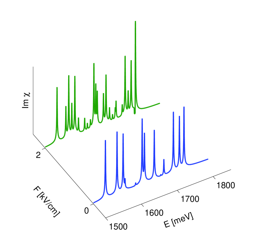
(a)

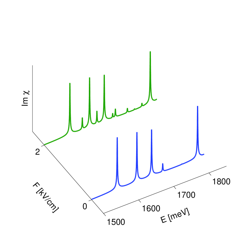
(b)

Figure 1: The imaginary part of the mean susceptibility form the eq. (41), for two GaAs/Ga_0.7Al_0.3As WPQWs, a) of thickness 51 nm, b) of thickness 32,5 nm

5 Results for GaAs/Ga_1-xAl_xAs Parabolic Quantum Well and discussion

The calculation of the WPQW electrooptical functions consists of several steps. First, we define the confinement energies $\hbar\omega_{e,h}$. To this end we choose a specific WPQW having in mind the experimental results of Miller et al.[56]. They obtained optical spectra for GaAs(Well)/Ga_0.7Al_0.3As (Barrier) QWs of three thicknesses: $L=51\pm\leavevmode\nobreak\ 3,5\leavevmode\nobreak\ \hbox{nm},L=32,5\pm\leavevmode\nobreak\ 3.5\leavevmode\nobreak\ \hbox{nm},L=33.6\pm\leavevmode\nobreak\ 3.5\leavevmode\nobreak\ \hbox{nm}$. We have performed the calculations for the thicknesses $L=51\leavevmode\nobreak\ \hbox{nm}$ and $L=32,5\leavevmode\nobreak\ \hbox{nm}$. The confinement parameters were obtained from the lowest energy levels of equivalent rectangular QWs with confinement potentials $V_{e,conf}=410.38\leavevmode\nobreak\ \hbox{meV},V_{h,conf}=72.42\leavevmode\nobreak\ \hbox{meV}$ [49].
The QWs energy states were obtained by standard methods (see, for example, Ref. [57] and [49] for calculation details), using the band parameters from Table 1. In the considered parabolic QW, the lowest energy levels are very similar to the case of an infinite, rectangular well, as one can see on the Fig. 2

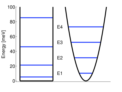
Figure 2: Comparison of the lowest energy levels in an infinite and parabolic QW, calculated from equation (8), for GaAs(Well)/Ga_0.7Al_0.3As (Barrier) and thickness $L=32.5\hbox{nm}$.

The values $a^{*}$, $R^{*}$ are appropriate for electrons and holes for the QW material, and are defined as

$$R^{*}=\frac{me^{4}}{2(4\pi\epsilon_{0}\epsilon_{b})^{2}\hbar^{2}},\,\,\,\,\,\,\,\,a^{*}=\frac{\hbar^{2}(4\pi\epsilon_{0}\epsilon_{b})}{me^{2}}.$$ (37)

The corresponding values, listed in Table 1, were obtained by using in (37) the appropriate effective masses: $m_{e}$ for $R^{*}_{e},a^{*}_{e}$, and $\mu_{\parallel H,L}$ for $R^{*}_{H},a^{*}_{H}$ and $R^{*}_{L},a^{*}_{L}$; $\mu_{\parallel H,L}$ are the in-plane reduced masses for the electron-hole pair and for the heavy- and light-hole exciton data.

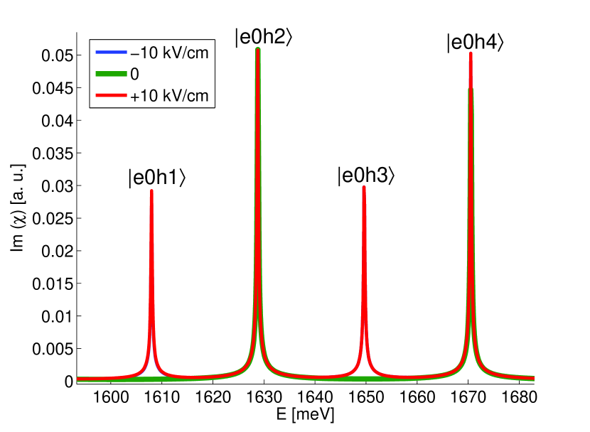
(a)

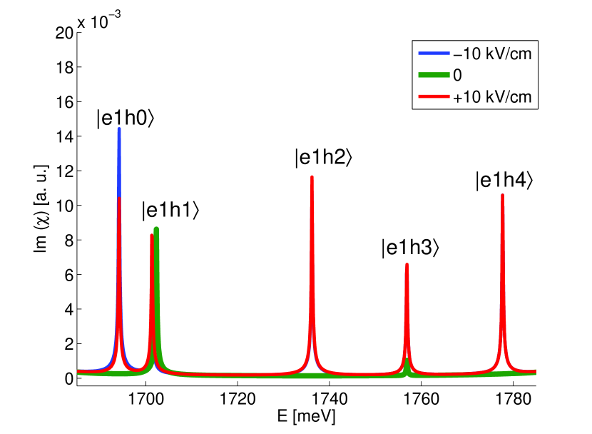
(b)

Figure 3: The imaginary part of the mean electrosusceptibility for the GaAs/Ga_0.7Al_0.3As WPQW of thickness 32.5 nm, for different energy intervals

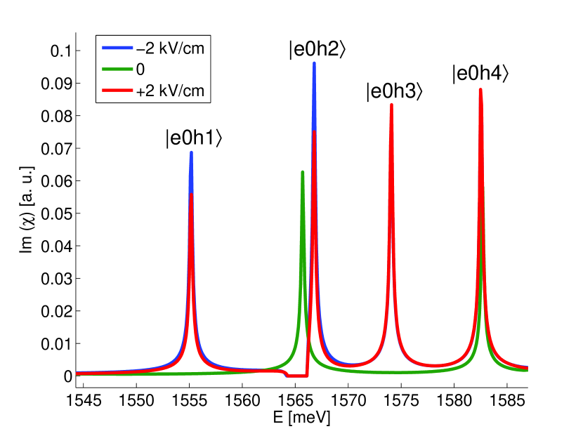
(a)

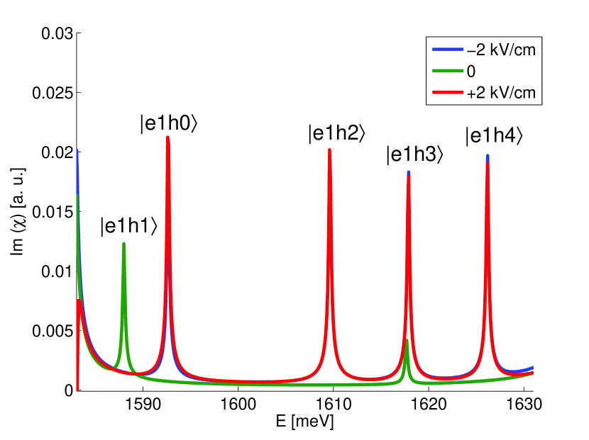
(b)

Figure 4: The same as in Fig. 3, for the WPQW of the thickness 51 nm

The results for the confinement energy states are displayed in Table 2. From this energies we obtained the confinement energies as

$$\hbar\omega_{e}=2E_{e0},\qquad\hbar\omega_{hH,L}=2E_{0zH,L}.$$ (38)

Table 2: Confinement parameters for the WPQWs from Ref. [56], dimensions in nm, energies in meV,

$L$	$\hbar\omega_{e}$	$\hbar\omega_{hH}$	$\hbar\omega_{hL}$	$E_{e0}$	$E_{0zH}$	$E_{0zL}$	$\alpha_{e}a_{H}^{*}$	$\alpha_{hH}a_{H}^{*}$	$\alpha_{hL}a_{L}^{*}$
32.5	81.66	19.74	108.4	40.83	9.87	54.2	4.21	4.95	4.76
51.5	43.56	8.46	34.4	21.78	4.23	17.2	3.07	3.08	2.68

Table 3: Confinement states accounted in computation

$|e0h0\rangle\rightarrow|1\rangle$	$|e0h1\rangle\rightarrow\rangle|2\rangle$	$|e0h2\rangle\rightarrow|3\rangle$	$|e0h3\rangle\rightarrow|4\rangle$	$|e0h4\rangle\rightarrow|5\rangle$
$|e1h0\rangle\rightarrow|6\rangle$	$|e1h1\rangle\rightarrow|7\rangle$	$|e1h2\rangle\rightarrow|8\rangle$	$|e1h3\rangle\rightarrow|9\rangle$	$|e1h4\rangle\rightarrow|10\rangle$
$|e2h0\rangle\rightarrow|11\rangle$	$|e2h1\rangle\rightarrow|12\rangle$	$|e2h2\rangle\rightarrow|13\rangle$	$|e2h3\rangle\rightarrow|14\rangle$	$|e2h4\rangle\rightarrow|15\rangle$
$|e3h0\rangle\rightarrow|16\rangle$	$|e3h1\rangle\rightarrow|17\rangle$	$|e3h2\rangle\rightarrow|18\rangle$	$|e3h3\rangle\rightarrow|19\rangle$	$|e3h4\rangle\rightarrow|20\rangle$
$|e4h0\rangle\rightarrow|21\rangle$	$|e4h1\rangle\rightarrow|22\rangle$	$|e4h2\rangle\rightarrow|23\rangle$	$|e4h3\rangle\rightarrow|24\rangle$	$|e4h4\rangle\rightarrow|25\rangle$

Using the above parameters and taking into account the lowest 25 confinement states (see Table 3) we have solved the eqn. (36) and obtained the coefficients $Y_{jn}$ from which we have determined the induced polarization inside the WPQW by the relation

$$P(z)=2M_{0}\psi_{0}(\rho_{0})\sum\limits_{j,n=0}^{N}|\hbox{e}j\hbox{h}n\rangle(z)Y_{jn},$$ (39)

with the notation

$$|\hbox{e}j\hbox{h}n\rangle(z)=\psi_{ej}(z)\psi_{hn}(z).$$ (40)

Having the polarization, we compute the mean dielectric susceptibility

$$\overline{\chi}=\pi\epsilon_{b}\psi_{0}(\rho_{0})\sum\limits_{\ell=0}^{N}\mathcal{Y}_{\ell}\langle 1|\ell\rangle_{\Lambda/2}$$ (41)

where $\langle 1|\ell\rangle_{\Lambda/2}=\frac{1}{\Lambda}\int\limits_{-\Lambda/2}^{\Lambda/2}|\ell\rangle(\zeta){\rm d}\zeta,\Lambda=\frac{L}{a^{*}}$, and the index $\ell$ runs over the 25 states listed in Table 3. Then, having the mean susceptibility, one can compute, using the appropriate boundary conditions, the optical functions (reflectivity, transmission, and absorption).

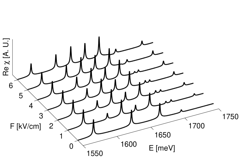
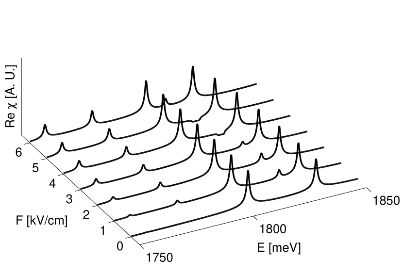
Figure 5: The real part of the mean electrosusceptibility for the GaAs/Ga_0.7Al_0.3As WPQWs of thicknesses 32.5 nm for different energy intervals and applied field strengths

We have computed the electrosusceptibility for two WPQWs of thicknesses $32.5\leavevmode\nobreak\ \hbox{nm}$ and $51\leavevmode\nobreak\ \hbox{nm}$. The parameters $S=2.6,\varpi=0.154$ and $v=0.5$ were determined with the procedure described in Ref. [50].

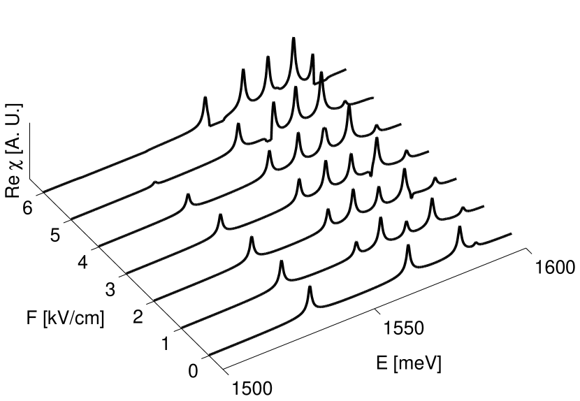
(a)

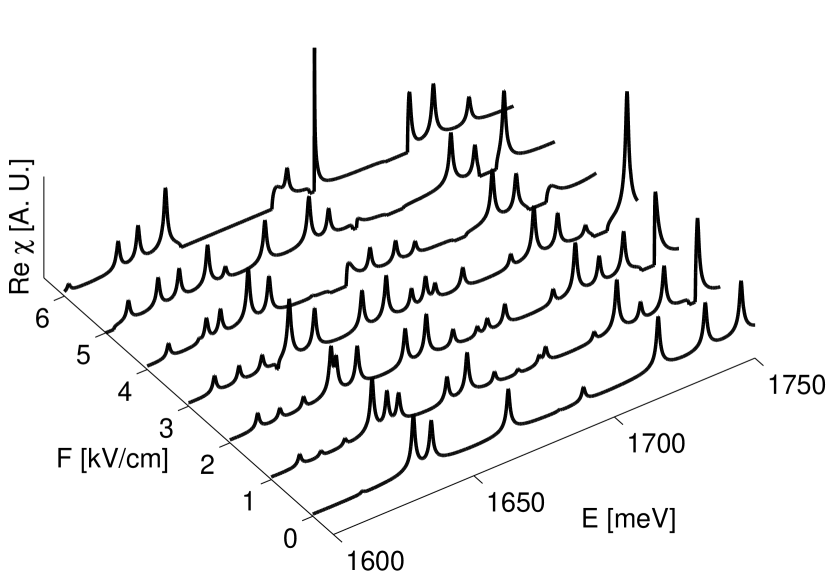
(b)

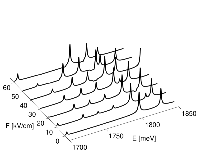
(c)

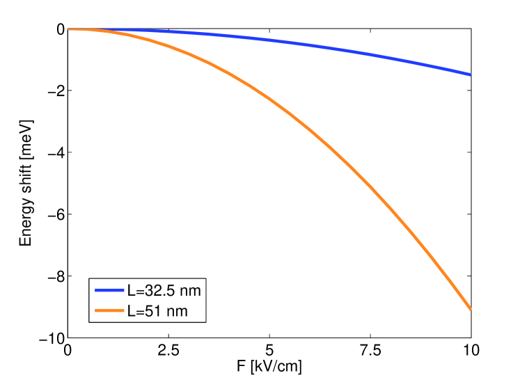
(d)

Figure 6: a), b) The real part of the mean electrosusceptibility for the GaAs/Ga_0.7Al_0.3As WPQWs of thickness 51 nm , for different energy intervals and applied field strengths. c) the impact of high electric fields (WPQW of thickness 32.5 nm) d) The comparison of the Stark energy shift of the two considered WPQWs for the lowest resonance.

Assuming a certain value of the coherence radius $\rho_{0}$, we have determined the lowest excitonic eigenfunction $\psi_{0}$. Finally, taking a certain value of the damping parameter $\mit\Gamma$, we have solved the constitutive equation (18), obtaining the coherent amplitudes. From the amplitudes we have computed the mean dielectric susceptibility (41). The advantage of the RDMA is that we obtain simultaneously the real and the imaginary part of the susceptibility. The results for the the imaginary part of the mean susceptibility of the considered WPQWs are displayed in Fig.1, Fig.2, and Fig.3. In Fig. 1 we show the general effect of the applied electric field for two GaAs/Ga_0.7Al_0.3As WPQws. We observe the red shift of the resonances, changes in the oscillator strengths, and the occurrence of new resonances due to the broken symmetry. The spectra for $F=0$ agree well with the experimental results by Miller et. al. [56] and our previous theoretical results [50]. In Fig. 2 and Fig. 3 we show the obtained spectra in a more detailed form, as compared to Fig. 1.

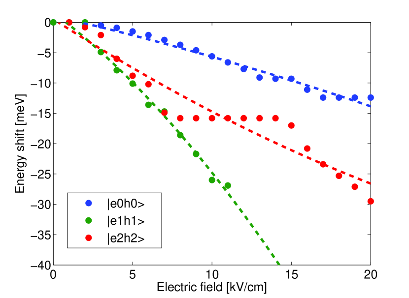
(a)

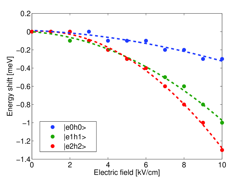
(b)

Figure 7: The Stark energy shift for the lowest resonances: (a)for the GaAs/Ga_0.7Al_0.3As WPQW of thickness 51 nm and (b) for the GaAs/Ga_0.7Al_0.3As WPQW of thickness 32.5 nm

In all the cases we observe changes in the placement of resonances, and the occurrence of new peaks attributed to different symmetries for the electron and the hole confinement functions. For high values of the applied electric field the effects are smaller which is due to the decreasing overlap of the electron and the hole confinement functions. We also observe that the shape of the spectra changes with the change of the direction of the applied field. Using the properties of the RDMA, we also obtained the real part of the mean electrosusceptibility, which is displayed in Fig.4 and Fig. 5a. The impact of high electric fields is displayed in Fig.5b, where we show the changes in the real part of the electrosusceptibility for the applied fields up to 60 kV/cm. Our method allows to determine the energy shift as a function of the applied field. We have computed the energy shift for the lowest confinement states. We observe the quadratic Stark shift for the lowest state and a more complicated field-dependence for higher states, as is displayed in Fig.6. Finally, we show that the energy shift drastically depends on the thickness of the QW (Fig.7), as was also observed for narrow QWs (see, for example, [6], [54] and references therein). Since the confinement energy depends on the QW thickness as $L^{-2}$, we see that for rectagular QW, $\Delta E=-CL^{4}$. The energy shift in the parabolic well on the Fig. 6(d) also closely follows this relation.

6 Conclusions

We have developed a simple mathematical procedure to calculate the electrooptical functions of Wide Parabolic Quantum Wells. Using the Real Density Matrix Approach and a model e-h interaction potential, we derived an analytical formula for the WPQW electrosusceptibility, from which another electrooptical functions can be obtained. The presented method has been used to investigate the electrooptical functions of GaAs/Ga_1-xAl_xAs WPQWs for the case of radiation incidence parallel to the growth direction. We have obtained the red shift of the resonances, changes in the oscillator strengths and new peaks related to electronic transitions forbidden for the case with absent electric field. We also observed the dependence of the spectra on the size of the QW and on the direction of the applied field. For the cases where the experimental data were available (for example, for WPQWs with F=0), we obtained a good agreement of our theoretical results with experiment. We hope that our results may stimulate experiments on Quantum Confined Stark Effect in WPQWs.

References

• [1] D. A. B. Miller, D. S. Chemla, T. C. Damen, A. C. Gossard, W. Wiegmann, T. H. Wood, C. A. Burrus, Phys. Rev. Lett. 53, 2173 (1984).
• [2] D. A. B. Miller, D. S. Chemla, T. C. Damen, A. C. Gossard, W. Wiegmann, T. H. Wood, C. A. Burrus, Phys. Rev. B. 32, 1043 (1985).
• [3] C. Alibert, S. Gaillard, J. A. Brum. G. Bastard, P. Frijlink, M. Erman, Solid State Commun. 53, 457 (1985).
• [4] E. J. Austin and M. Jaros, J. Phys. C: Solid State Phys. 18, L 1091 (1985).
• [5] D. A. B. Miller, D. S. Chemla, and S. Schmidt-Rink: Phys. Rev. B 33, 6976 (1986).
• [6] H.-J.Polland, K. Köhler, L. Schultheis, J. Kuhl, E. O. Göbel, and C. W. Tu, Superlatt. Microstruct. 2, 309 (1986).
• [7] L. Schultheiss, K. Köhler, and C. W. Tu, Phys. Rev. B 36, 6609 (1987).
• [8] Z. Ikonić, V. Milanović, and D. Tjapkin, J. Phys. C: Solid State Phys. 20, 1147 (1987).
• [9] A. P. Thorn, A. J.Shields, P. C. Klipstein, N. Apsley, and T. M. Kerr, J. Phys. C: Solid State Phys. 20, 4229 (1987).
• [10] A. Shimizu, Phys. Rev. B 37, 8527 (1988).
• [11] Jia-Lin Zhu, Dao-Hua Tang, and Jia-Jiong Xiong, Phys. Rev. B 39, 8609 (1989).
• [12] L. Viña, M. Potemski, J. C. Maan, G. E. W. Bauer, E. E. Mendez, W. I. Wang, Superlatt. Microstruct. 3, 371 (1989).
• [13] I. Galbraith and G. Duggan, Phys. Rev. B 40, 5515 (1989).
• [14] H. Shen, M. Dutta, L. Fotiadis, P. G. Newman, R. P. Moerkirk, W. H. Chang, and R. N. Sacks, Appl. Phys. Lett. 57, 2118 (1990).
• [15] P. W. Yu, D. C. Reynolds, G. D. Sanders, K. K. Bajaj, C. E. Stutz, and K. R. Evans, Phys. Rev. B 43, 4344 (1991).
• [16] C. Weisbuch and B. Vinter, Quantum Semiconductor Structures. Fundamentals and Applications (Academic Press, San Diego, CA, 1991).
• [17] S. Jaziri, G. Bastard, and R. Bennaceur, J. de Physique IV, Colloque C.5, supplement au J. de Physique 11, Vol. 3, 367 (1993).
• [18] R. Goldhahn, S. Shokhovets, D. Schultze, N. Stein, S. Gobsch, T. S. Cheng, M. Henini, and J. M. Chamberlain, Superlatt. and Microstruct. 15, 119 (1994).
• [19] R. André, J. Cibert, and Le Si Dang, Phys. Rev. B 52, 12013 (1995).
• [20] J. Kavaliauskas, G. Krivaité, A. Galickas, I. Simkené, U. Olin, and M. Ottosson, Phys. Stat. Sol. B 191, 155 (1995).
• [21] K. Kuo, H. Zheng, S. Xu, P. Zhang, W. Zhang, and X. Yang, Appl. Phys. Lett. 67, 2642 (1995).
• [22] S. W. Short, S.H. Xin, A. Yin, H. Luo, M. Dobrowolska, and J.K. Furdyna, J. of Electronic Materials 25, 253 (1996).
• [23] P. V. Giugno, M. De Vittorio, R. Rinaldi, R. Cingolani, F. Quaranta, L. Vanzetti, L. Sorba, and A. Franciosi, Phys. Rev. B 54, 16934 (1996).
• [24] K. Tanaka, N. Kotera,and H. Nakamura, Electronic Letters 34, 2163 (1998).
• [25] E. Schöll, Tr. J. of Physics 23, 635(1999).
• [26] G. Czajkowski and L. Silvestri, Electric and magnetic field effects on optical properties of excitons in semiconductor nanostructures, in Electrons and photons in solids - A volume in honour of Franco Bassani, edited by G.  Grosso, G. C. La Rocca and M.  Tosi (Scuola Normale Superiore - Pubblicazioni della classe di scienze, Pisa, Italy, 2001), pp. 271-288.
• [27] K. Tanaka, T. Murata, N. Kotera,and H. Nakamura, Superlatt. and Microstruct. 29, 91 (2001).
• [28] M. Larsson, P. O. Holtz, A. Elfving, G. V. Hansson, and W.-X. Ni, Phys. Rev. B 71, 113301 (2005).
• [29] A. John Peter, K. Gnanasekar, and K. Navaneethakrishnan, Eur. Phys. J. B 53, 283 (2006).
• [30] E. Sari, S. Nizamoglu, T. Ozel, and H. Volkan Demira, Appl. Phys. Lett. 90, 011101 (2007).
• [31] G. Czajkowski and Ł. Skowroński, Adv. Studies Theor. Phys. 1, 187 (2007).
• [32] J. W. Robinson, J. H. Rice, K. H. Lee, J. H. Na, R. A. Taylor, D. G. Hasko, R. A. Oliver, M. J. Kappers, C. J. Humphreys, and G. A. D. Briggs, Appl. Phys. Lett. 86, 213103 (2005).
• [33] H. Masui, J. Sonoda, N. Pfaff, I. Koslow, S. Nakamura and S. P. DenBaars, J. Phys. D: Appl. Phys. 41, 165105 (2008).
• [34] F. Stokker-Cheregi, A. Vinattieri, E. Feltin, D. Simeonov, J. Levrat, J.-F. Carlin, R. Butt , N. Grandjean, and M. Gurioli, Appl. Phys. Lett. 93, 152105 (2008).
• [35] J.-H. Ryou, P. Douglas Yoder, J. Liu, Z. Lochner, H. Kim, S. Choi, H. Jin Kim, and R. D. Dupuis, IEEE J. of Selected Topics in Quantum Electronics, 15, 1080 (2009).
• [36] S. Baskoutas and A. F. Terzis, Eur. Phys. J. B 69, 237 (2009).
• [37] R. Leitsmann and F. Bechstedt, Phys. Rev. B 80, 165402 (2009).
• [38] F. Dujardin, E. Feddi, E. Assaid, and A. Oukerroum, Eur. Phys. J. B 74, 507 (2010).
• [39] D. Camacho Mojica and Yann-Michel Niquet, Phys. Rev. B 81, 195313 (2010).
• [40] A. Miteva, Trakia Journal of Sciences 8, Suppl. 3, 1 (2010).
• [41] J. Lähnemann, O. Brandt, C. Pfüller, T. Flissikowski, U. Jahn, E. Luna, M. Hanke, M. Knelangen, A. Trampert, and H. T. Grahn, Phys. Rev. B 84, 155303 (2011).
• [42] V. A. Harutyunyan, and V. A. Gasparyan, Micro and Nanosystems 5, 61 (2013).
• [43] S. Barthel1,K. Schuh, O. Marquardt, T. Hickel, J. Neugebauer, F. Jahnke, and G. Czycholl, Eur. Phys. J. B 86, 449 (2013).
• [44] S. Ramanathan, G. Petersen, K. Wijesundara, R. Thota, E. A. Stinaff, M. L. Kerfoot, M. Scheibner, A. S. Bracker, and D. Gammon, Appl. Phys. Lett. 102, 213101 (2013).
• [45] J. Wilkes and E. A. Muljarov, arXiv:1502.07094v1 [cond-mat.mes-hall] 25. Feb. 2015.
• [46] A. Tabata, M. R. Martins, J. B. B. Oliveira, T. E. Lamas, C. A. Duarte, E. C. F. da Silva, and G. M. Gusev, J. Appl. Phys. 102, 093715 (2007).
• [47] A. Tabata, J. B. B. Oliveira, E. C. F. da Silva, T. E. Lamas, C. A. Duarte, and G. M. Gusev, J. Phys. Conf. Series 210, 012052 (2010).
• [48] A. Taqi and J. Diouri, Semicon.Phys., Quantum Electronic and Optoelectronics 15, 21 (2012).
• [49] G. Czajkowski, S. Zielińska-Raczyńska, D. Ziemkiewicz, http://arxiv.org/abs/1502.05329 (2015).
• [50] G. Czajkowski, S. Zielińska-Raczyńska, D. Ziemkiewicz, Eur. Phys. J. B, accepted (2015).
• [51] P. Schillak, European Phys. Journ. B 84 17 (2011).
• [52] A. Stahl and I. Balslev, Electrodynamics of the Semiconductor Band Edge (Springer-Verlag, Berlin-Heidelberg-New York, 1987).
• [53] G. Czajkowski, F. Bassani, and A. Tredicucci, Phys. Rev. B 54, 2035 (1996).
• [54] G. Czajkowski, F. Bassani, and L. Silvestri, Rivista del Nuovo Cimento 26, 1-150 (2003).
• [55] I. S. Gradshteyn and I. M. Ryzhik, Table of Integrals, Series, and Products, 5th ed., ed. by A. Jeffrey (Academic Press, Boston, 1994).
• [56] R. C. Miller, A. C. Gossard, D. A.Kleinman, and  O. Munteanu, Phys. Rev. B 29, 3740 (1984).
• [57] J. H. Davies, The Physics of Low-Dimensional Semiconductors (University Press Cambridge, 1998).
• [58] M. Grundmann, O. Stier, and D. Bimberg, Phys. Rev. B 52, 11969 (1995).