Comparison of the calorimetric and kinematic methods
of neutrino energy reconstruction in disappearance experiments

Abstract

To be able to achieve their physics goals, future neutrino-oscillation experiments will need to reconstruct the neutrino energy with very high accuracy. In this work, we analyze how the energy reconstruction may be affected by realistic detection capabilities, such as energy resolutions, efficiencies, and thresholds. This allows us to estimate how well the detector performance needs to be determined a priori in order to avoid a sizable bias in the measurement of the relevant oscillation parameters. We compare the kinematic and calorimetric methods of energy reconstruction in the context of two $\nu_{\mu}\rightarrow\nu_{\mu}$ disappearance experiments operating in different energy regimes. For the calorimetric reconstruction method, we find that the detector performance has to be estimated with an $\mathcal{O}(10\%)$ accuracy to avoid a significant bias in the extracted oscillation parameters. On the other hand, in the case of kinematic energy reconstruction, we observe that the results exhibit less sensitivity to an overestimation of the detector capabilities.

I Introduction

Long-baseline experimental searches of neutrino oscillations largely rely on the capability of pinning down the energy dependence of the oscillation probability, which is a nontrivial function of the true neutrino energy, $E_{\nu}$. As a consequence, the procedure employed to reconstruct the unknown incoming-neutrino energy from the measured kinematics of the interaction products is a central element of the oscillation analysis.

Experiments using neutrino beams peaked at $E_{\nu}\sim 600$–800 MeV, such as T2K ref:T2K and MiniBooNE ref:MiniBooNE , determine the energy distribution of charged-current (CC) events from the kinematics of the outgoing charged lepton—i.e., its kinetic energy and emission angle—measured by large Cherenkov detectors filled with water or mineral oil. This technique is mostly applied to quasielastic (QE) events—identified by the absence of pions in the final state—that provide the dominant contribution to the total cross section at these energies. However, it necessarily involves hypotheses on the reaction mechanism.

The kinematic method of energy reconstruction is based on the assumptions that the beam particle interacts with a single nucleon at rest, bound with constant energy, and that no other nucleons are knocked out from the nucleus. It has been long known, however, that processes involving two-nucleon currents, final-state interactions, and nucleon-nucleon correlations give rise to the appearance of more complex final states, featuring more than one nucleon excited to the continuum. Reconstruction of the neutrino energy of such events, dubbed QE-like in the mesonless case ref:Martini_QElike , in general requires more complex methods, involving realistic models of nuclear dynamics.

At energies well above 1 GeV, the contribution of inelastic processes—resonant pion production and deep-inelastic scattering (DIS)—becomes larger and eventually dominant. As a consequence, determination of the neutrino energy in this kinematic region requires reconstruction of events with many hadrons in the final state.

As alternative to Cherenkov detectors in this regime, calorimeters measuring the visible energy associated with each event—i.e., the energy deposited by the final-state particles—have been proposed as effective devices, allowing for an accurate neutrino-energy reconstruction. Calorimeters are presently being used in the MINOS ref:MINOS and NO$\nu$A ref:NOvA experiments. In their detectors, the total energy deposited by all reaction products is measured without a prior reconstruction of each final-state particle’s track, momentum, or energy. The energy response for potentially complex final states is calibrated using test-beam exposures.

On the other hand, future appearance experiments like DUNE ref:LBNE are expected to employ detectors capable of fine-grained tracking of a large number of interaction products. In their case, the tracking capability is the key to being able to select electron-neutrino events and distinguish them from backgrounds, even for non-QE events.

In this article, we compare the kinematic and calorimetric reconstruction methods in the oscillation analysis of a $\nu_{\mu}$ disappearance experiment. We also aim to explore the capabilities and limitations of a calorimetric analysis based on individually identified particle tracks and to determine what level of understanding of detector response and underlying events is required to meet certain physics goals.

For a muon-neutrino event, it is clear that the long muon track in itself is a clear signature, and no tracking beyond the leading muon is required for backgrounds removal. However, we study the $\nu_{\mu}$ disappearance channel because of its simplicity in terms of oscillation physics, and as a sandbox to develop suitable analysis tools.

The calorimetric technique, as defined above, obviously rests on the ability of fully reconstructing the final state, which largely depends on the detector design and performance. Nuclear effects also play a role, as they may lead to a sizeable amount of missing energy, hindering the reconstruction of $E_{\nu}$. For example, if a pion produced at the elementary interaction vertex is absorbed in the spectator system, in general, its energy is not deposited in the calorimeter.

We consider an idealized setting, in which the near and far detectors are functionally identical, and a simple extrapolation between them can be performed ref:Gallagher . To minimize the uncertainty arising from nuclear interactions, the target nucleus selected for both detectors is carbon, the cross section of which has been extensively measured in a number of different channels ref:NOMAD_inclusive ; ref:NOMAD ; ref:SciBooNE_inclusive ; ref:MINERvA_anu ; ref:MiniB_NC ; ref:MiniB_CCQE_nu ; ref:MiniB_piC ; ref:MiniB_pi0 ; ref:T2K_CC_numu_xsec_C ; ref:MINERvA_nu ; ref:MiniB_CCQE_anu ; ref:T2K_CC_numu_xsec_CH ; ref:T2K_CCQE_numu_xsec_C ; ref:T2K_CCQE_numu_C ; ref:T2K_CC_nue ; ref:MiniB_NCQE_anu ; ref:MINERvA_nu_p ; ref:MINERvA_CC_ratios ; ref:MINERvA_coherent_piC ; ref:MINERvA_piC ; ref:MINERvA_pi0 .

The analyzed events are generated using the simulation code genie ref:GENIE supplemented with the $\nu T$ package of additional modules ref:vT , allowing us to describe the carbon ground state using the realistic spectral function ref:Omar_LDA .

To cover different experimental configurations, we consider two options: a low-energy (LE) setup, with a narrow-band off-axis beam, and a high-energy (HE) setup, featuring a broadband on-axis beam. In the LE option, the neutrino flux is peaked around 600 MeV, and the distance to the far detector is set to $L=295$ km, while in the HE option, the flux is peaked at $\sim$1–2 GeV and $L=1000$ km.

Event reconstruction is carried out assuming:

1. a perfect scenario, in which all produced particles are detected and their true energies are measured,

2. a realistic one, in which detection efficiencies and thresholds are taken into account and the finite detector resolution leads to a smearing of the measured energies.

In both cases, neutrons are assumed to escape detection altogether.

A key element of our analysis is the migration matrices, the elements of which, ${\mathcal{M}}_{ij}$, correspond to the probability that an event with a true neutrino energy in the $j$th bin ends up being reconstructed in an energy bin $i$.

The event distribution representing the data is in each case generated using the realistic scenario. Fitted rates, on the other hand, are obtained using a linear combination of migration matrices corresponding to the perfect and realistic scenarios. This procedure is very effective from the computational point of view, and provides a measure of the impact of detector performance on the oscillation-parameters fit.

This article is structured as follows. In Sec. II we derive different methods of neutrino-energy reconstruction, placing a special emphasis on the approximations involved. The neutrino cross section model employed for event generation and the treatment of detector effects are outlined in Secs. III and IV, respectively. In Sec. V, we discuss the calculated migration matrices. Our oscillation analysis and its results are presented in Sec. VI. Finally, in Sec. VII, we summarize our findings.

II Energy reconstruction methods

Consider CC neutrino scattering off a nuclear target, resulting in the knockout of $n$ nucleons and production of $m$ mesons. The energy and momentum conservation can be cast in the form

$$E_{\nu}+M_{A} = E_{\ell}+E_{A-n}+\sum_{i}E_{{\mathbf{p}}_{i}^{\prime}}+\sum_{j}E_{{\mathbf{h}}_{j}^{\prime}},$$ (1)

$$\mathbf{k}_{\nu} = \mathbf{k}_{\ell}-\mathbf{p}+\sum_{i}\mathbf{p}^{\prime}_{i}+\sum_{j}\mathbf{h}^{\prime}_{j},$$ (2)

respectively, where $E_{\nu}$ and $\mathbf{k}_{\nu}$ ($E_{\ell}$ and $\mathbf{k}_{\ell}$) are the neutrino’s (charged lepton’s) energy and momentum, $E_{{\mathbf{p}}_{i}^{\prime}}$ and $\mathbf{p}^{\prime}_{i}$ denote the energy and momentum of the $i$th knocked-out nucleon ($1\leq i\leq n$), and $E_{{\mathbf{h}}_{j}^{\prime}}$ and $\mathbf{h}^{\prime}_{j}$ stand for the energy and momentum of the $j$th produced meson ($1\leq j\leq m$). The energy of the residual $(A-n)$-nucleon system, $E_{A-n}$, can be conveniently expressed as

$$E_{A-n}=M_{A}-nM+E+T_{A-n},$$ (3)

in terms of the nucleon (target-nucleus) mass $M$ ($M_{A}$), the recoil energy $T_{A-n}$, and the excitation energy $E$. In Eq. (2), the recoil momentum of the system is denoted as $-\mathbf{p}$, to allow the interpretation of $\mathbf{p}$ as the vector sum of the initial momenta of the knocked-out nucleons, assuming that it is not altered by final-state interactions with the residual system.

Substitution of Eq. (3) into Eq. (1) leads to the neutrino energy in the form

$$E_{\nu}=E_{\ell}+E+T_{A-n}+\sum_{i}(E_{{\mathbf{p}}_{i}^{\prime}}-M)+\sum_{j}E_{{\mathbf{h}}_{j}^{\prime}}.$$ (4)

Note that while for mesons the total energies enter the sum, for nucleons only the kinetic energies contribute. This difference is a consequence of the fact that mesons are produced in the interaction process, whereas nucleons are only knocked out from the target nucleus.

Assuming that multinucleon effects do not introduce strong energy dependence to the cross sections, the factor $\epsilon_{n}=E+T_{A-n}$ can be treated as a constant at neutrino energies above several hundred MeV. Then, reconstruction of the neutrino energy reduces to determining the energies of the particles in the final state ref:MINOS_PRL ,

$$E^{\textrm{cal}}_{\nu}=\epsilon_{n}+E_{\ell}+\sum_{i}(E_{{\mathbf{p}}_{i}^{\prime}}-M)+\sum_{j}E_{{\mathbf{h}}_{j}^{\prime}}.$$ (5)

This, so-called, calorimetric method can, in principle, be applied to any type of CC interaction. However, one needs to keep in mind that an accurate reconstruction of hadrons poses a formidable experimental challenge. In particular, neutrons typically escape detection, and any undetected meson results in energy underestimation by at least the value of the pion mass, $\sim$135 MeV.

When the invariant hadronic mass squared, defined as

$$W^{2}=\Big{(}\sum_{i}E_{{\mathbf{p}}_{i}^{\prime}}+\sum_{j}E_{{\mathbf{h}}_{j}^{\prime}}\Big{)}^{2}-\Big{(}\sum_{i}\mathbf{p}^{\prime}_{i}+\sum_{j}\mathbf{h}^{\prime}_{j}\Big{)}^{2},$$

is known, Eqs. (1) and (2) can be solved for the neutrino energy, yielding the alternative expression ref:Omar&Davide

$$E_{\nu}=\frac{2E_{\mathbf{p}}E_{\ell}-2\mathbf{p}\cdot\mathbf{k}_{\ell}+W^{2}-(E_{\mathbf{p}}^{2}-\mathbf{p}^{2})-m_{\ell}^{2}}{2(E_{\mathbf{p}}-|\mathbf{p}|\cos\theta_{N}-E_{\ell}+|\mathbf{k_{\ell}}|\cos\theta)},$$ (6)

where $E_{\mathbf{p}}=M_{A}-E_{A-n}$, $m_{\ell}$ is the charged lepton’s mass, $|\mathbf{p}|\cos\theta_{N}=\mathbf{p}\cdot\mathbf{k}_{\nu}/E_{\nu}$, and $|\mathbf{k_{\ell}}|\cos\theta=\mathbf{k}_{\ell}\cdot\mathbf{k}_{\nu}/E_{\nu}$.

On the other hand, in the case of a single-nucleon knockout associated with the production of $m$ mesons, the requirement that the nucleon is on the mass shell, $E_{{\mathbf{p}^{\prime}}}^{2}=M^{2}+\mathbf{p}^{\prime 2}$, can be used to obtain the neutrino energy as

$$E_{\nu}={\frac{M^{2}+(\mathbf{p}-\mathbf{k}_{\ell}-\sum_{j}\mathbf{h}^{\prime}_{j})^{2}-(E_{\mathbf{p}}-E_{\ell}-\sum_{j}E_{{\mathbf{h}}_{j}^{\prime}})^{2}}{2\big{[}E_{\mathbf{p}}-|\mathbf{p}|\cos\theta_{N}-E_{\ell}+|\mathbf{k_{\ell}}|\cos\theta-\sum_{j}{\mathcal{H}}_{j}\big{]}}},$$ (7)

with ${\mathcal{H}}_{j}=E_{{\mathbf{h}}_{j}^{\prime}}-\mathbf{h}^{\prime}_{j}\cdot\mathbf{k}_{\nu}/E_{\nu}$.

In practice, an application of the above formulas requires (i) neglecting the unmeasured recoil momentum $|\mathbf{p}|$ and (ii) approximating the energy of the residual nuclear system by a constant, which amounts to setting $E_{\mathbf{p}}=nM-\epsilon_{n}$ in Eq. (6) and $E_{\mathbf{p}}=M-\epsilon$ in Eq. (7). These simplifications lead to the expressions

$$E_{\nu}^{\textrm{kin}}=\frac{2(nM-\epsilon_{n})E_{\ell}+W^{2}-(nM-\epsilon_{n})^{2}-m_{\ell}^{2}}{2(nM-\epsilon_{n}-E_{\ell}+|\mathbf{k_{\ell}}|\cos\theta)},$$ (8)

and

$$E_{\nu}^{\textrm{mt}}=\frac{M^{2}+(\mathbf{k}_{\ell}+\sum_{j}\mathbf{h^{\prime}_{j}})^{2}-(M-\epsilon-E_{\ell}-\sum_{j}E_{{\mathbf{h}}_{j}^{\prime}})^{2}}{2(M-\epsilon-E_{\ell}+|\mathbf{k_{\ell}}|\cos\theta-\sum_{j}{\mathcal{H}}_{j})}.$$ (9)

Owing to difficulties with an accurate determination of the invariant hadronic mass, the use of Eq. (8) is usually restricted to the process of a single-nucleon knockout with no pions produced, in which $W^{2}$ is known and equals $M^{2}$ ref:K2K_PRL ; ref:MiniB_kappa ; ref:NOMAD ; ref:SciBooNE_inclusive ; ref:MINERvA_anu . On the other hand, Eq. (9) has been applied in the energy reconstruction for single-pion events by the MiniBooNE Collaboration ref:MiniB_piC , setting the single-nucleon separation energy $\epsilon$ to zero.

The kinematic energy reconstruction, by means of Eq. (8) or (9), does not require the knocked-out nucleon’s momentum to be measured. However, as this method assumes specific final states, its accuracy is spoiled by any undetected hadron. For example, when a produced pion is absorbed or undetected, the energy reconstructed from Eq. (8) under the QE hypothesis is typically lower than the true one by $\sim$300–350 MeV; see Figs. 6 and 7 of Ref. ref:Leitner . While the process of multinucleon knockout affects the energy reconstruction in a similar way—i.e., it redistributes the strength of the reconstructed flux from the peak mainly to the low-energy tail ref:Martini_Erec1 ; ref:Martini_Erec2 —this effect seems to be less relevant at higher beam energies ref:Lalakulich_Erec .

For completeness, we mention that neutrino energy can be also found exploiting momentum conservation only. Equation (2) multiplied by a factor $\mathbf{k}_{\nu}/E_{\nu}$,

$$E_{\nu}=|\mathbf{k_{\ell}}|\cos\theta-|\mathbf{p}|\cos\theta_{N}+\sum_{i}|{\bf p}^{\prime}_{i}|\cos\theta_{i}+\sum_{j}|{\bf h}^{\prime}_{j}|\cos\theta_{j},$$ (10)

where $|{\bf p}^{\prime}_{i}|\cos\theta_{i}=\mathbf{p}^{\prime}_{i}\cdot\mathbf{k}_{\nu}/E_{\nu}$ and $|{\bf h}^{\prime}_{j}|\cos\theta_{j}=\mathbf{h}^{\prime}_{j}\cdot\mathbf{k}_{\nu}/E_{\nu}$, shows that $E_{\nu}$ can be determined from the projections of the final momenta on the beam direction. Neglecting the contribution of the recoil momentum, one obtains the expression

$$E^{\textrm{mom}}_{\nu}=|\mathbf{k_{\ell}}|\cos\theta+\sum_{i}|{\bf p}^{\prime}_{i}|\cos\theta_{i}+\sum_{j}|{\bf h}^{\prime}_{j}|\cos\theta_{j},$$ (11)

a special case of which has been employed in an analysis of single-nucleon knockout events by the NOMAD Collaboration ref:NOMAD .

Performing the kinematic energy reconstruction in this article, we employ Eq. (8) assuming single-nucleon knockout, regardless of the actual number of nucleons in the final state. We set $W^{2}$ to $M^{2}$ for mesonless events and to $M_{\Delta}^{2}$, $M_{\Delta}=1.232$ GeV being the $\Delta$ resonance mass, when at least one meson is observed. The single-nucleon separation energy is fixed to 34 MeV. The same value of $\epsilon$ is added in the calorimetric energy reconstruction (5) for every nucleon detected.

III Event generation

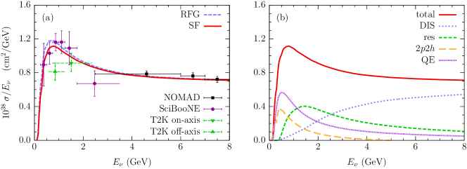
Figure 1: (color online). Panel (a): Per-nucleon CC inclusive $\nu_{\mu}$ cross section divided by neutrino energy, obtained using genie $2.8.0+\nu$T ref:GENIE ; ref:vT with the relativistic Fermi gas model (dashed line) and the spectral function approach (solid line) as a nuclear model in QE interaction. The results for carbon are compared to the experimental data for carbon extracted from NOMAD ref:NOMAD_inclusive and those for hydrocarbon (CH) reported from SciBooNE ref:SciBooNE_inclusive and T2K ref:T2K_CC_numu_xsec_C ; ref:T2K_CC_numu_xsec_CH . Panel (b): Breakup of the contributions to the inclusive cross section. The labels DIS, res, $2p2h$, and QE refer to deep-inelastic scattering, resonant pion production, two-nucleon knockout, and quasielastic scattering, respectively.

Our analysis is based on the description of nuclear structure and interaction dynamics in the genie Monte Carlo generator ref:GENIE , version 2.8.0, supplemented with the $\nu T$ package of additional modules ref:vT .

genie is a modern and versatile platform for neutrino event simulation. It has been developed putting special emphasis on scattering in the energy region of few GeV—important for ongoing and future oscillation studies—where various mechanism of interaction are relevant. A number of neutrino experiments employs this generator in data analysis ref:Dytman_NuFact10 .

Resonant pion production in genie, considered for $W\leq 1.7$ GeV, is accounted for using the model of Rein and Sehgal ref:Rein&Sehgal . Compared to 18 in the original model, 16 resonances of unambiguous existence are implemented using up-to-date parameters but neglecting the interference between them. The effect of the charged lepton’s mass is taken into account only in the calculations of the phase-space boundaries.

The contribution of nonresonant processes, classified in genie as DIS, is calculated following the method of Bodek and Yang ref:Bodek&Yang ; ref:Bodek&Yang_updated . This effective approach extends the range of applicability of the parton model to low neutrino energy by modifying the (leading-order) parton-distribution functions in the low-$Q^{2}$ region, $Q^{2}$ being the four-momentum transfer squared. Higher-order and target-mass corrections are accounted for by replacing Bjorken $x$ with a new scaling variable ref:Bodek&Yang ; ref:Bodek&Yang_updated . While DIS in genie is the only mechanism of interaction at $W>1.7$ GeV, it also produces one- and two-pion events in the resonance region.

Hadronization in genie is performed using the Andreopoulos–Gallagher–Kehayias–Yang approach ref:AGKY , which combines Koba–Nielsen–Olesen (KNO) scaling ref:KNO at low values of the hadronic invariant mass with the pythia/jetset calculations ref:PYTHIA at high $W$, ensuring a smooth transition between the two regimes.

Two-nucleon knockout ($2p2h$) events are simulated in genie using the procedure of Dytman ref:GENIE_2p , obtained modifying and extending the one of Ref. ref:Lightbody&OConnell , derived for electron scattering. The invariant mass of two-nucleon events is assumed to have a Gaussian distribution centered at $W=(M+M_{\Delta})/2$. The charged lepton’s kinematics is distributed according to the magnetic contribution to the cross section for scattering on a free nucleon ref:LlewellynSmith , identical for neutrinos and antineutrinos. The strength, adjusted to fit the cross sections reported by MiniBooNE ref:MiniB_CCQE_nu ; ref:MiniB_CCQE_anu , is implemented to linearly decrease to zero for the neutrino energy between 1 and 5 GeV, to avoid inconsistency with the results from NOMAD ref:NOMAD . As the experimental data constrain the two-nucleon contribution for the carbon target only, for other nuclei its strength is assumed to exhibit linear dependence on the mass number $A$.

In QE scattering, the default nuclear model in genie is the relativistic Fermi gas (RFG) model of Bodek and Ritchie ref:Bodek&Ritchie , in which a high-momentum tail—inspired by the effects of nucleon-nucleon correlations—is added to the nucleon momentum distribution.

Using the $\nu T$ package ref:vT , we replace the RFG model by the spectral function (SF) approach ref:Omar_RMP , the implementation of which has been validated through comparisons with electron-scattering data. In the SF formalism, the interaction between the beam particle and the nucleus is assumed to involve a single nucleon, with the remaining $(A-1)$ nucleons acting as spectators. Under this assumption—called the impulse approximation—the target initial state can be described by the nuclear spectral function $P(\mathbf{p},E)$, giving the probability distribution that removal of a nucleon with momentum $\mathbf{p}$ from the nuclear ground state leaves the residual $(A-1)$-nucleon system with excitation energy $E$.

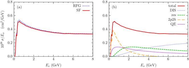
Figure 2: (color online). Same as in Fig. 1 but for the muon antineutrino.

The realistic SF of carbon, employed in the $\nu T$ package, has been obtained by the authors of Ref. ref:Omar_LDA in the local-density approximation (LDA). The LDA scheme relies on the premise that surface and shell effects do not affect short-range correlations between nucleons in nuclei, and it is supported by the evidence that for $|\mathbf{p}|\gtrsim 300$ MeV the momentum distribution is largely independent of the mass number $A$, for nuclei with $A\geq 4$ ref:Omar_RMP . Therefore, using the LDA, the correlation contribution to the nuclear SF can be obtained from theoretical calculations for uniform nuclear matter at different densities ref:Omar_NM ; ref:Omar_LDA and consistently combined with the shell structure of the nucleus, deduced from experimental $(e,e^{\prime}p)$ data ref:Saclay_C ; ref:Dutta . We stress that the carbon SF of Ref. ref:Omar_LDA has proven successful in describing electron-scattering data in various kinematical setups, see e.g. Ref. ref:FSI , and the momentum distribution obtained from it is consistent with the one extracted from $(e,e^{\prime}p)$ data at large missing energy and momentum ref:Rohe .

The effect of using the $\nu T$ package on the total inclusive CC cross section for muon neutrinos in genie is presented in Fig. 1. On the one hand, the SF calculation of the QE cross section improves the agreement with the experimental data at low energies reported by the SciBooNE Collaboration ref:SciBooNE_inclusive . On the other hand, it does not alter the good agreement at the kinematics of the NOMAD experiment ref:NOMAD_inclusive , where the inclusive cross section is dominated by the contributions of DIS processes and resonant pion production; see Fig. 1. Note that in the case of the NOMAD data, the error bars represent $\Delta(\sigma/E_{\nu})$, whereas for the SciBooNE points, they correspond to $(\Delta\sigma)/E_{\nu}$ ref:SciBooNE_inclusive .

While the calculations do not seem to reproduce the SciBooNE point at the average neutrino energy of 2.47 GeV, it is important to note that its energy range extends over the whole high-energy tail of the flux and does not end at 3.5 GeV.

The recent results of the T2K experiment ref:T2K_CC_numu_xsec_C ; ref:T2K_CC_numu_xsec_CH suggest that in the $\sim$1 GeV region uncertainties of the inclusive cross section may be sizable, of the order of 20%, and that the contribution of the $2p2h$ processes may be smaller than that deduced from MiniBooNE. Should the $2p2h$ estimate be significantly reduced in genie, the calculated cross sections would be in very good agreement with the T2K data.

For the sake of completeness, in Fig. 2, we show the total inclusive CC cross section for muon antineutrinos, for which experimental data are not available. It clearly appears that the $2p2h$ contribution—which in genie ref:GENIE_2p is assumed to be the same for neutrinos and antineutrinos—plays a much more important role in the latter case.

As this article is focused on the effects of realistic detection capabilities on energy reconstruction, we leave comparisons to exclusive cross sections for future studies of nuclear-model uncertainties of the results presented here. Being able to reproduce the inclusive cross sections—of minimal uncertainties—the employed description of neutrino interactions can be deemed suitable for the purpose of this analysis.

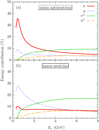
Figure 3: (color online). Fraction of the (a) $\bar{\nu}_{\mu}$ and (b) $\nu_{\mu}$ energy converted into the kinetic energies of neutrons (solid lines) and protons (dotted lines) and the total energies of charged (short dashed lines) and neutral (long dashed lines) pions.

In the context of the calorimetric energy reconstruction, it is important to estimate how different species of hadrons contribute to the final-state energy. In Fig. 3, we present the obtained fraction of the $\bar{\nu}_{\mu}$ and $\nu_{\mu}$ energy carried out by neutrons, protons, and pions.

While at energies below $\sim$1 GeV the neutron results for neutrinos and antineutrinos clearly differ, this is not the case when DIS and resonant pion production become the dominant reaction mechanisms. Having in mind the numerical uncertainties—estimated not to exceed 1%—we conclude that at $E_{\nu}\gtrsim 1.5$ GeV neutrons contribute less than 15% of the (anti)neutrino energy.

As can be expected from QE interactions, the contribution of protons in neutrino interactions resembles that of neutrons in antineutrino scattering and vice versa. For antineutrinos, the knocked-out protons carry out less than 10% of the initial energy in the whole considered region. However, for neutrinos, the protons contribution is much more sizable and reduces to $\leq 10$% for energies exceeding $\sim$3.35 GeV.

Although the total energies of $\pi^{0}$’s enter the calorimetric energy reconstruction, in the considered kinematic range, their contributions are smaller than that of neutrons. On the other hand, in the region dominated by resonant and nonresonant pion production, charged pions give the largest contribution to the final-state hadronic energy.

We observe that at energies above 0.5 GeV the analogical results for electron neutrinos and antineutrinos do not differ significantly from those presented in Fig. 3.

IV Considered detector effects

In our analysis, two extreme sets of assumptions are considered regarding the detector performance:

• Perfect reconstruction.
  With the exception of neutrons, all produced particles are observed, and their measured energies are equal to the true ones.

• Realistic setup.
  The measured energies and angles are smeared with respect to the true ones by a finite detector resolution. The detection efficiencies and thresholds are taken into account. Neutrons are assumed to escape detection.

The detection thresholds applied in our calculations correspond to the measured kinetic energy of 20 MeV for mesons and 40 MeV for protons. For comparison, the NOMAD and MiniBooNE experiments were able to detect protons of kinetic energy above $\sim$50 MeV ref:NOMAD , and the $\sim$40-MeV threshold is expected for future liquid-argon detectors Barger:2007yw .

The efficiencies are treated as energy independent, for the sake of simplicity, and set to 60% for $\pi^{0}$’s, 80% for other mesons, and 50% for protons. Those values can be considered rather optimistic, compared to the efficiencies achieved in existing detectors ref:NOMAD ; ref:efficiency_pi0_ND280 ; ref:efficiency_piC_MINERvA . We assume that produced charged leptons are always detected.

Accounting for the effect of finite detector resolution on an observable $x_{\textrm{meas}}$, we smear it according to the Gaussian distribution centered at the true value $x_{\textrm{true}}$,

$$f(x_{\textrm{meas}})=\frac{1}{\sqrt{2\pi}\sigma(x_{\textrm{true}})}\exp\left[-\frac{1}{2}\left(\frac{x_{\textrm{meas}}-x_{\textrm{true}}}{\sigma(x_{\textrm{true}})}\right)^{2}\right].$$

In the case of the muon, we apply this procedure to the momentum and production angle, using

$$\sigma(|\mathbf{k_{\mu}}|)=0.02|\mathbf{k_{\mu}}|\quad\textrm{ and }\quad\sigma(\theta)=0.7^{\circ},$$ (12)

as in the MINERvA experiment ref:MINERvA . For the electron, the realistic resolutions ref:MiniB_nue ; ref:NOvA

$$\sigma(E_{e})=0.10E_{e}\quad\textrm{ and }\quad\sigma(\theta)=2.8^{\circ}$$ (13)

are used.

For other particles, the only smeared quantity is the energy. To the electromagnetic showers produced by $\pi^{0}$ decays, we employ the energy resolution given by

$$\frac{\sigma(E_{\pi^{0}})}{E_{\pi^{0}}}=\max\left\{\frac{a_{\pi^{0}}}{\sqrt{E_{\pi^{0}}}},\,\frac{b_{\pi^{0}}}{E_{\pi^{0}}}\right\}$$ (14)

with $a_{\pi^{0}}=0.107$ and $b_{\pi^{0}}=0.02$, while for other hadrons,

$$\frac{\sigma(E_{h})}{E_{h}}=\max\left\{\frac{a_{h}}{\sqrt{E_{h}}},\,b_{h}\right\}$$ (15)

is used with $a_{h}=0.145$ and $b_{h}=0.067$. The values of $\sigma$ and the energies appearing in Eqs. (14) and (15) are expressed in units of GeV. Note that the hadron-energy resolutions applied in our analysis can be considered optimistic, as they are to be compared to

$$\frac{\sigma(E_{\pi^{0}})}{E_{\pi^{0}}}=2\sqrt{\frac{a_{\pi^{0}}^{2}}{E_{\pi^{0}}}+\frac{b_{\pi^{0}}^{2}}{E_{\pi^{0}}^{2}}}\quad\textrm{and}\quad\frac{\sigma(E_{h})}{E_{h}}=2\sqrt{\frac{a_{h}^{2}}{E_{h}}+b_{h}^{2}}$$

achieved in the MINOS ref:MINOS and MINERvA ref:MINERvA experiments. Note that the assumed $\pi^{+}$ energy resolution is also optimistic when compared with the expectation for future liquid-argon detectors from Ref. Stahl:2012exa .

It is important to emphasize that in the context of the kinematic method of energy reconstruction our assumptions are conservative. We employ realistic detector resolutions for muons and make minimal use of information on observed hadrons. Disregarding additional protons in the final state, we reconstruct every event as if it involved single-nucleon knockout. All mesons in the final state are assumed to originate from a single resonance of the invariant mass $M_{\Delta}=1.232$ GeV, and their angular distributions are not taken into account; compare to Eq. (9). On the other hand, detector effects entering the calorimetric method are treated in a rather optimistic way, compared to those in existing detectors.

Note that knocked-out neutrons are assumed to be undetected both in the realistic and perfect scenarios, owing to difficulties of their reconstruction in neutrino events. Traveling some distance from the primary interaction vertex before scattering, neutrons are currently problematic to associate with the neutrino event, and they typically deposit only part of their energy in the detector. However, this assumption may need to be revisited in the future, when an ongoing experimental program Berns:2013usa ; Liu:2015fiy brings important progress in the understanding of the detector response to neutrons.

V Migration matrices

In our calculations, detector effects are taken into account in the migration matrices, $\mathcal{M}^{X}_{ij}$, the columns of which are the probability distribution functions (PDFs) for a neutrino interaction $X$ at the true energy in the $i$th bin to be reconstructed with an energy in the $j$th bin. The observed event distribution can then be calculated as

$$N^{\textrm{tot}}_{i}=\sum_{X}\sum_{j}\mathcal{M}^{X}_{ij}N^{X}_{j},$$

where $X$ runs over the four types of interactions considered (DIS, res, $2p2h$, and QE), $i$ and $j$ refer to the energy bins, and $N^{X}_{j}$ stands for the number of $X$ events in the bin $j$ computed without detector effects. Note that, barring the boundary effects, the smearing produced by the migration matrices does not have any impact on the total number of events.

To facilitate the reproduction of our results, we provide the complete set of migration matrices, calculated for the energies up to 8 GeV, using 0.1 GeV bins, and the cross sections employed in our analysis matricesRef .

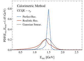
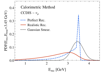
Figure 4: (color online). Probability distribution functions for a $\nu_{\mu}$ event of the energy $E_{\textrm{true}}$ to be reconstructed at an energy $E_{\textrm{rec}}$. The results obtained for a QE event at $E_{\textrm{true}}=1.45$ GeV (top) and a DIS event at $E_{\textrm{true}}=3.45$ GeV (bottom) show the effects of different assumptions on the detector performance; see the text for details.

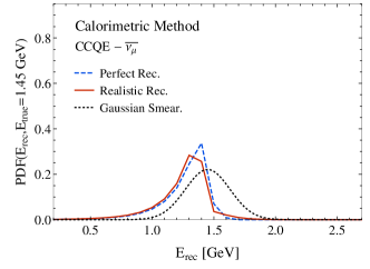
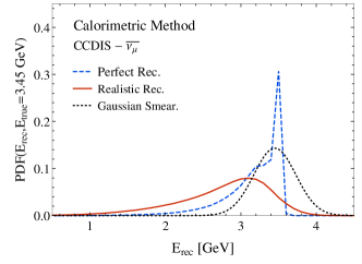
Figure 5: (color online). Same as in Fig. 4 but for a $\bar{\nu}_{\mu}$ event.

In an ideal detector, all migration matrices would be the unit matrices. In a real experiment, the reconstructed energy may depend on the reconstruction procedure, as well as on the mechanism of interaction. Imperfect detection capabilities—energy resolutions, efficiencies, and thresholds for particle detection—affect the probability for a neutrino event to be reconstructed in the correct energy bin. In particular, finite energy resolutions smear the measured energies, while imperfect efficiencies and finite thresholds result in an energy partially carried away by undetected particles. As a consequence, PDFs have finite widths, they are asymmetric, with a broader tail toward the lower energies, and their mean values are lowered with respect to the true neutrino energies.

Those features are illustrated in Figs. 4 and 5 for the QE (DIS) mechanism of interaction and the true neutrino and antineutrino energy of 1.45 GeV (3.45 GeV) reconstructed using the calorimetric method. Comparing the PDFs obtained for the perfect and realistic reconstructions, defined in Sec. IV, one can observe how sizable the effect of realistic detector capabilities is. For reference, we also show the Gaussian distribution with the standard deviation $\sigma(E_{\nu})=0.15\sqrt{E_{\nu}}$, with $\sigma$ and $E_{\nu}$ in units of GeV, typically applied to account for detector effects in phenomenological studies devoted to liquid-argon detectors Barger:2007yw ; ref:LBNE ; Agarwalla:2012bv ; Agarwalla:2013qfa ; Agarwalla:2011hh .

The differences between the neutrino and antineutrino PDFs can be traced back to a twofold reason: (i) different contributions of neutrons to the final-state energy, as shown in Fig. 3, and (ii) the typical energy transfer being lower in antineutrino interactions, owing to the destructive interference of the response functions.

Even for the perfect-reconstruction scenario, the PDFs are asymmetric, as a consequence of pion absorption in the nuclear medium and the energy carried out by neutrons, assumed to escape detection. When the realistic detector effects are accounted for, the PDFs clearly broaden due to the employed energy resolutions, and their modes shift toward lower energies. The latter effect is particularly large for DIS events, in which the muon contribution to the final-state energy is typically smaller than in QE scattering, and the role of the efficiencies is larger.

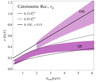
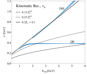
Figure 6: (color online). Effective energy resolution as a function of the true energy for muon neutrinos. The results of our Monte Carlo simulations for QE (DIS) events are shown as lower (upper) bands. For each band, the upper (lower) edge corresponds to the realistic (perfect) detection capabilities, defined in Sec. IV. For comparison, a few smearing functions frequently used in phenomenological oscillation studies are also shown.

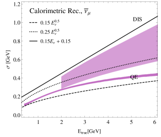
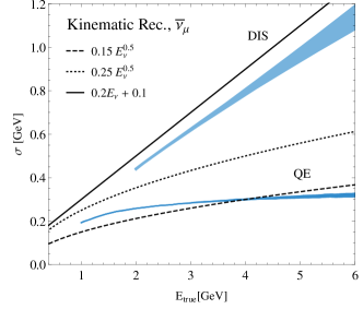
Figure 7: (color online). Same as in Fig. 6 but for $\bar{\nu}_{\mu}$’s.

To make contact with existing phenomenological studies of neutrino and antineutrino oscillations, in Figs. 6 and 7, we compare a few simple functions typically employed as an effective energy resolution with our estimates based on the Monte Carlo simulations, for both the calorimetric (upper panels) and kinematic (lower panels) reconstruction methods. Our calculations of the PDF’s standard deviations are presented as bands spanning the values between the results for the perfect-reconstruction scenario (lower edge) and those for the realistic scenario (upper edge). The estimates for QE and DIS events are shown separately, as the lower (darker) and upper (lighter) bands. Because the energy resolutions applied in the realistic scenario exceed those in existing experiments roughly two times, they can be considered optimistic. On the other hand, an effective energy resolution higher than our result for the perfect-reconstruction scenario does not seem to be possible to achieve without the reconstruction of neutrons.

Note that for liquid-argon experiments (such as DUNE or LBNO) or totally active scintillator detectors (e.g., NO$\nu$A), the effective energy resolution is typically assumed to be $\sigma(E_{\nu})=\mathcal{O}(0.05\textrm{--}0.2)\sqrt{E_{\nu}}$, in units of GeV; see, for instance, Refs. Barger:2007yw ; Patterson:2012zs ; ref:LBNE ; Agarwalla:2012bv ; Agarwalla:2011hh ; Agarwalla:2013qfa . On the other hand, for experiments based on the Cherenkov technique (such as T2K), the resolution $\sigma(E_{\nu})=\mathcal{O}(0.08)\sqrt{E_{\nu}}$ is usually applied in phenomenological studies Huber:2009cw ; Agarwalla:2013qfa .

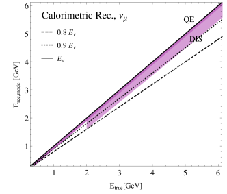
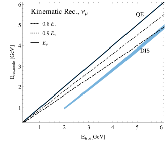
Figure 8: (color online). Mode of the reconstructed-energy distributions as a function of the true energy calculated for muon neutrinos. The bands show our Monte Carlo results, with the lower (upper) edge obtained assuming the realistic (perfect-reconstruction) scenario. The darker (lighter) bands present the results for QE (DIS) events. For reference, the lines corresponding to the true value and its underestimation by 10 and 20% are also shown.

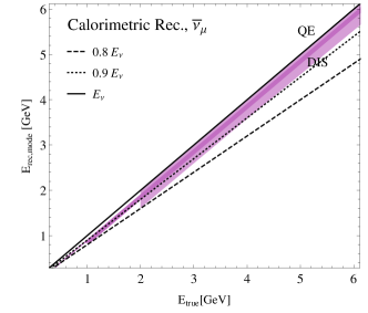
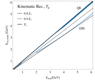
Figure 9: (color online). Same as in Fig. 8 but for $\bar{\nu}_{\mu}$’s.

Finally, in Figs. 8 and 9, we show how the modes of the reconstructed-energy distributions depend on the true value of energy, comparing the calorimetric and kinematic reconstruction methods. The bands represent our Monte Carlo results for QE and DIS events, the lower (upper) edge of which corresponds the realistic (perfect-reconstruction) scenario.

In the calorimetric method, the modes for QE scattering are in a good agreement with the true energy, and the expected presence of neutrons in the final state of antineutrino events introduces only a small effect. While for DIS, the agreement is somewhat reduced—especially when detector effects are taken into account—the modes do not differ from the true energy by more than 20%.

For the kinematic method, in QE interactions, both the neutrino and antineutrino modes are in excellent agreement with the true energy. However, this is not the case for DIS events. For antineutrinos, the discrepancy between the DIS mode and the true energy exceeds 10% and is typically close to 20%. For neutrinos, the mode underestimates the true energy by $\sim$1 GeV. This behavior can be traced back to the simplicity of our kinematic analysis, assuming that all events containing at least one pion are produced through excitation of a resonance of the invariant mass $M_{\Delta}=1.232$ GeV; see Eq. (8). Should an experiment be able to reconstruct pions angles with high angular resolution, more refined treatment (9) would be possible.

The bands in Figs. 6–9 show the differences between the results for the realistic and perfect-reconstruction scenarios. Their widths can be used as a measure of the sensitivity to detector effects, which turns out to be larger for the calorimetric migration matrices than for the kinematic ones. However, they do not represent uncertainties entering any actual experiment. In practical situations, detection capabilities and their uncertainties are estimated in test-beam exposures. In Sec. VI, we are going to analyze the importance of an accurate estimate of these uncertainties in the context of an oscillation analysis.

VI Oscillation analysis

The event number expected in a neutrino-energy bin, without considering detector effects, can be computed as

$$N^{i}_{\beta}=\int_{E_{\nu}^{i}}^{E_{\nu}^{i}+\Delta E_{\nu}}dE_{\nu}\>\sigma_{\nu_{\beta}}(E_{\nu})\>P_{\alpha\beta}\left(\{\Theta\},E_{\nu}\right)\>\phi_{\nu_{\alpha}}(E_{\nu}),$$ (16)

where the indices $\alpha$ and $\beta$ label the initial and final neutrino flavors, respectively; $\Delta E_{\nu}$ is the energy-bin size; $\sigma_{\nu_{\beta}}$ denotes the ${\nu_{\beta}}$ cross section; and $\phi_{\nu_{\alpha}}$ is the unoscillated $\nu_{\alpha}$ flux. The $\nu_{\alpha}\rightarrow\nu_{\beta}$ oscillation probability, $P_{\alpha\beta}$, depends on a set of oscillation parameters $\left\{\Theta\right\}$ as well as on the neutrino energy $E_{\nu}$. In the $\nu_{\mu}\rightarrow\nu_{\mu}$ oscillation channel, the oscillation probability can be approximated by

$$P_{\mu\mu}\simeq 1-\sin^{2}\theta_{\mu\mu}\sin^{2}\left(\frac{\Delta m^{2}_{\mu\mu}L}{4E_{\nu}}\right),$$

where

$$\sin^{2}\theta_{\mu\mu}=4\cos^{2}\theta_{13}\sin^{2}\theta_{23}(1-\cos^{2}\theta_{13}\sin^{2}\theta_{23}),$$

and $\Delta m^{2}_{\mu\mu}$ is the weighted average of $\Delta m_{31}^{2}$ and $\Delta m_{32}^{2}$ Nunokawa:2005nx that can be expressed as

$$\Delta m^{2}_{\mu\mu}=\Delta m^{2}_{31}+\mathcal{O}(\Delta m^{2}_{21}).$$

Should the experimental information on the $E_{\nu}$ distribution of events be available, the values of the oscillation parameters $\{\Theta\}$ could be, in principle, directly inferred from the data However, modern neutrino beams are produced as tertiary products, originating predominantly from the decay of pions and kaons produced in interactions of protons impinging on a target. Therefore, neutrinos are not monoenergetic, and—for a given event—the incident neutrino energy has to be reconstructed from the kinematics of the particles in the final state. Systematic uncertainties of this procedure inevitably depend on the capabilities of the employed detector, as well as on the neutrino interaction channel, owing to the different detection efficiencies for the particles involved in the event. Because for muons the efficiency uncertainty is minimal, its effect on the reconstructed energy spectrum is neglected in our analysis.

The kinematic method of energy reconstruction—used, for instance, in Cherenkov detectors—is known to be accurate to $\sim$100–150 MeV for QE events ref:Ankowski_NuFact2014 . However, as discussed in Sec. II, this is not the case for the events of QE topology containing undetected hadrons. For example, a single undetected pion typically spoils the reconstructed energy by $\sim$300–350 MeV ref:Leitner . For pion-production events, playing an important role at higher energies, either the accuracy is reduced [see Eq. (8) containing $W^{2}$, unknown on event-by-event basis] or detailed angular information is required [see Eq. (9)].

Phenomenological analyses for wide-band neutrino beams operating in the multi-GeV energy regime have shown that the sensitivity to neutrino oscillation parameters of a liquid-argon detector is similar to that of a Cherenkov detector of the mass $\sim$3–6 times larger, because of the lower efficiency of the latter for non-QE events Barger:2007yw ; Akiri:2011dv ; Huber:2010dx ; Coloma:2012ut ; Coloma:2012ma . It has been argued that the reason lies in the imaging capabilities of the liquid-argon technology, able to identify protons in addition to lepton tracks Barger:2007yw , as opposed to Cherenkov detectors in which the information on CC events comes predominantly from the charged leptons. Nevertheless, in such comparisons, the neutrino energy resolution at liquid-argon detectors was always assumed to be extremely good, in the range of $\sigma(E_{\nu})=0.15\sqrt{E_{\nu}}$. Should this be affected by detector effects, or by the energy carried away by unobserved particles, such conclusions may have to be reexamined.

In this work, we compare the kinematic and calorimetric methods of neutrino energy reconstruction in the context of a $\nu_{\mu}$ disappearance experiment. Four types of CC neutrino interactions are considered—resonant and nonresonant pion production, two-nucleon knockout, and quasielastic scattering—and modeled according to genie with the $\nu T$ package, as described in Sec. III. The coherent channel has not been taken into account because of its negligible contribution to the event rate ref:Formaggio . For each interaction type and both reconstruction methods, we have calculated corresponding migration matrices $\mathcal{M}^{X}_{ij}$ with and without detector effects; see Secs. IV and V.

In the $\nu_{\mu}\rightarrow\nu_{\mu}$ oscillation channel, the main background comes from neutral current events misidentified as CC ones. As it is generally expected to be very low, for simplicity, we neglect it in our analysis. On the other hand, due to the large event statistics, systematic uncertainties are expected to be relevant. In their treatment, we follow that of Refs. ref:Pilar_PRL ; ref:Pilar_PRD , with the $\chi^{2}$ implementation as detailed in the appendices of Refs. ref:Pilar_PRD ; ref:Coloma:2012ji . A 20% bin-to-bin uncorrelated systematic uncertainty is assumed, as well as a 20% overall normalization uncertainty, which is bin-to-bin correlated. The pull method is used, adding a Gaussian prior for each systematic error, and the final $\chi^{2}$ profile is obtained after the minimization over the nuisance parameters. These (rather conservative) systematic uncertainties are introduced in our analysis in order to accommodate possible differences in the shape of the expected event distributions at the detectors, in a similar fashion as was done in Refs. ref:Pilar_PRL ; ref:Pilar_PRD . A near detector is also considered in the analysis, which helps to constrain the nuisance parameters during the fit.

The oscillation analysis is performed using a modified version ref:Coloma:2012ji of globes GLB1 ; GLB2 . The assumed true values of the oscillation parameters are

$$\Delta m^{2}_{21}=7.50\times 10^{-5}\;\textrm{eV}^{2};\quad\Delta m^{2}_{31}=2.46\times 10^{-3}\;\textrm{eV}^{2};$$

$$\theta_{12}=33.48^{\circ};\quad\theta_{23}=42.30^{\circ};\quad\theta_{13}=8.50^{\circ};\quad\delta_{CP}=0.$$

(17)

In the analysis, we focus on the determination of atmospheric parameters $\theta_{23}$ and $\Delta m^{2}_{31}$. For simplicity, all oscillation parameters have been fixed during the analysis; i.e., no marginalization has been performed when obtaining the allowed confidence regions. However, our conclusions are not expected to change significantly if marginalization was performed within the currently allowed experimental regions. Matter effects are included in our simulations, and the matter density profile has been chosen according to the preliminary reference Earth model ref:PREM .

VI.1 Considered experimental setups

Oscillation experiments using neutrino beams produced from meson decays in flight can be divided into two main categories according to their far detector locations: on-axis (such as K2K ref:K2K and MINOS ref:MINOS and also the DUNE ref:LBNE and LAGUNA-LBNO ref:LBNO proposals) and off-axis (for instance, ongoing T2K ref:T2K and NO$\nu$A ref:NOvA ).

Because of the pion-decay kinematics, the flux at an off-axis site is well localized around a given neutrino energy, with the beam spread and high-energy tail heavily reduced ref:off-axis . Such a design allows for a significant reduction of the backgrounds coming from neutral-current events, and guarantees that the range of values of $L/E_{\nu}$ is well localized around the first oscillation maximum. The price to pay is a lower beam intensity compared to an on-axis configuration. In addition, as the mean neutrino energy is lower than in an on-axis experiment, the number of events in the far detector is also lower, since the cross section is an increasing function of the energy.

On the other hand, in an on-axis neutrino oscillation experiment, the spread of the beam is larger. In principle, this allows one to determine the shape of the oscillation probability by performing measurements at different values of $L/E_{\nu}$. In addition, thanks to the higher beam intensity and higher neutrino energies, large event statistics is easier to collect. As a consequence of being more energetic, though, the event sample generally contains a significant fraction of pion-production events. In addition, the high-energy tail typically produces a significant neutral-current background contaminating in particular the low-energy bins.

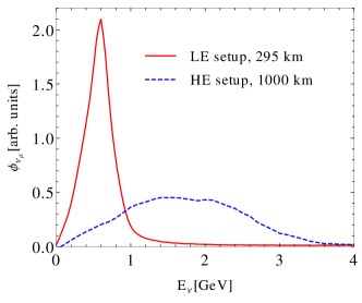
Figure 10: (color online). The muon neutrino fluxes (in arbitrary units) as a function of the neutrino energy for the two configurations considered in this work. The solid (dashed) line corresponds to the low-(high-)energy setup.

In this article, we perform an analysis of two different neutrino-oscillation experiments: a HE setup with a broadband on-axis beam, and a LE setup with a narrow-band off-axis beam.

In the LE setup, we use the neutrino beam of Ref. ref:Patrick2009 , being a preliminary estimate of that in the T2K experiment with the $2.5^{\circ}$ off-axis configuration ref:T2K_flux . As shown in Fig. 10, it is peaked at around 600 MeV. For the distance to the far detector for the LE setup, we take 295 km, the length corresponding to the first oscillation maximum. The normalization (i.e., number of protons on the target, detector size, and data-taking time) is arbitrarily set to obtain a total unoscillated CC inclusive event sample of $\mathcal{O}(5000)$ events in the energy range between 0.3 and 2 GeV, relevant to the analysis.

Table 1: Expected number of unoscillated CC $\nu_{\mu}$ events for the low- and high-energy setups defined in the text. In addition to the total event numbers, their breakup into different reaction mechanisms, labeled as in Fig. 1, is also given.

	QE	$2p2h$	res	DIS	total
LE (0.3–2 GeV)	49%	28%	21%	2%	4891
HE (0.3–4 GeV)	26%	11%	37%	26%	4456

For the HE option, the neutrino flux labeled as “650 km” in Ref. ref:Longhin is used, being one of the configurations considered within the LAGUNA design study ref:LAGUNA . This flux has a broad peak between $\sim$1 and $\sim$2 GeV, with a non-negligible tail extending well above 3 GeV; see Fig. 10. We considered several choices for the distance to the far detector in the range $L=\mathcal{O}(500\textrm{--}1000)$ km, for which the first oscillation maximum would lie within the energy range of the flux peak, and found that $L\sim 1000$ km gives optimal results in the $\nu_{\mu}$ disappearance channel. In the following, we discuss our results for this baseline choice only.

Since in this work we are only interested in exploring detector effects on different energy-reconstruction methods, the normalization for the HE setup is arbitrarily set to obtain a similar total number of unoscillated events as for the LE setup. However, due to the much higher neutrino energies, the composition of the inclusive event sample is very different. To illustrate it, the total number of unoscillated CC inclusive events at the far detector are given in Table 1 for both setups, together with the percentages for QE, $2p2h$, res and DIS events in each sample.

In our analysis, all neutrino events with the energies between 0.2 and 8 GeV are calculated for both LE and HE setups. However, only those which are reconstructed between 0.3 and 2 GeV (4 GeV) for the LE (HE) setup are considered during the fit. The $\chi^{2}$ is built by binning the events in reconstructed neutrino energy, using 100 MeV bins.

VI.2 Results for the calorimetric method

As explained in Sec. II, in the calorimetric method, the neutrino energy is reconstructed by adding the energies of all observed particles in the final state, and no information on the direction of the outgoing particles is used.

In an analysis of an oscillation experiment, one has to rely on a Monte Carlo simulation to predict the “expected” (or “fitted”) event rates. One of the inputs to such a simulation is detailed information on the detector capabilities. However, it is subject to uncertainties, the role of which we are going to analyze.

Our results for the calorimetric method are shown in Figs. 11 and 12 for the LE and HE setups, respectively. In their upper panels, we present the simulated event distributions in the far detector as a function of the reconstructed energy. The lower panels illustrate the confidence regions for fits to the atmospheric oscillation parameters. In the fits, the true event rates are computed for the oscillation parameters (17) taking into account detector effects according to the realistic setup described in Sec. IV.

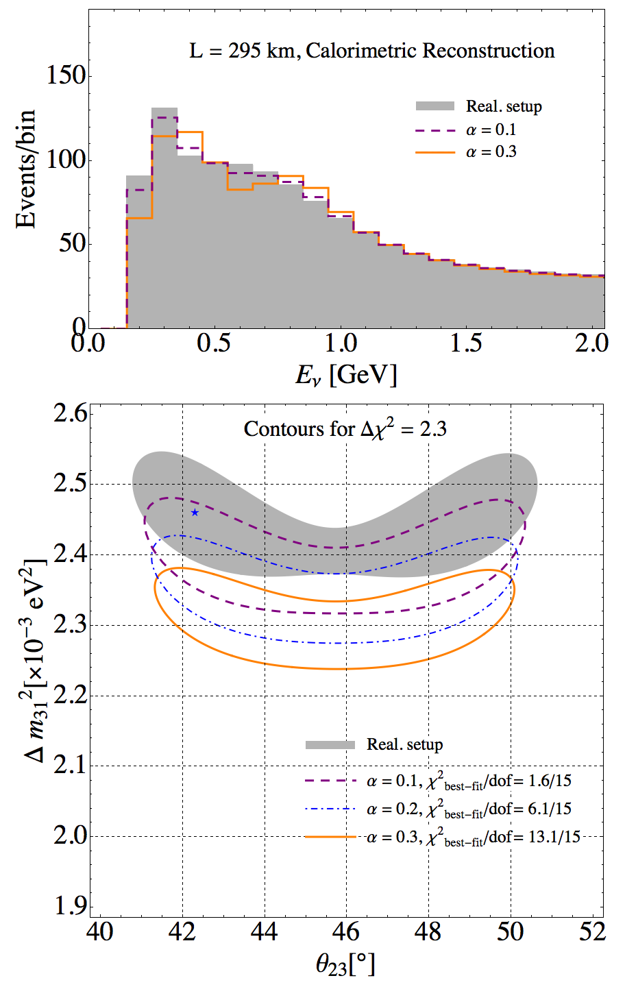
Figure 11: (color online). Results for the low-energy setup and the calorimetric reconstruction method. Upper panel: Simulated charged-current event distributions in the far detector as a function of the reconstructed energy, for the oscillation parameters (17). The shaded histogram corresponds to a perfect estimate of detector effects (see Sec. IV). The dashed and solid lines show the event rates obtained with the detector performance overestimated by 10% and 30%. Lower panel: Confidence regions in the $(\theta_{23},\Delta m^{2}_{31})$ plane, at 1$\sigma$ C.L. (2 degrees of freedom). The shaded area corresponds to the perfect estimate of the detector effects. The lines show the contours obtained for the detector performance overestimated by 10%, 20%, and 30% in the fit. The star indicates the true values of the oscillation parameters, the same for all confidence regions shown.

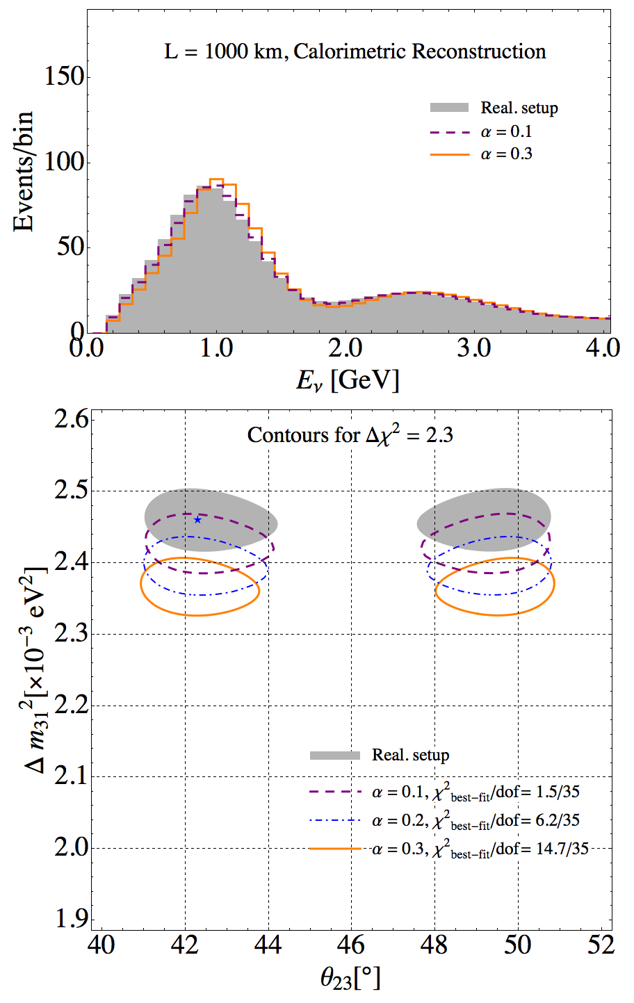
Figure 12: (color online). Same as in Fig. 11 but for the high-energy setup and the calorimetric reconstruction method.

Because it is computationally expensive to generate a given set of migration matrices from simulated neutrino events, in our analysis, the fitted rates are generated using a linear combination of the matrices obtained for the realistic and perfect-reconstruction scenarios. Allowing for a continuous transformation of the event-rate distribution from one scenario to the other, this method is useful to quantify when the incorrect estimation of the detector performance starts to have a significant impact on the fit. In practice, the fitted rates are obtained as:

$$N_{i}^{\textrm{fit}}=\sum_{X}\sum_{j}\left\{(1-\alpha)M^{X,\textrm{ real}}_{ij}+\alpha M_{ij}^{X,\textrm{ perf}}\right\}N^{X}_{j},$$ (18)

where $X$ stands for a given type of interaction (QE, $2p2h$, res, or DIS) and $i$ and $j$ are the energy-bin indices. $M^{X,\textrm{ real}}$ and $M^{X,\textrm{ perf}}$ denote the migration matrices obtained for the realistic and perfect-reconstruction scenarios, respectively. Finally, $N^{X}_{j}$ is the event rate in the energy bin $j$ for the interaction type $X$, computed without accounting for the detector effects, as in Eq. (16).

In Eq. (18), $\alpha$ is a purely phenomenological parameter, used to obtain the “effective” migration matrices as a linear deformation of the two extreme scenarios under consideration. For instance, $\alpha=0$ means that the fitted rates are obtained in the same way as the true rates. On the other hand, $\alpha=0.3$ means that the fitted rates are obtained underestimating the role of detector effects by 30%, a substantial amount. Two examples of the event distributions obtained for different values of $\alpha$ are shown in the upper panels in Figs. 11 and 12. Even though the distributions look very different, all histograms have been obtained assuming the same true values for the oscillation parameters (17).

For a given value of $\alpha$, the fitted rates are simulated for every possible combination of $(\Delta m^{2}_{31},\theta_{23})$. The point in the $(\Delta m^{2}_{31},\theta_{23})$ plane which gives a best fit to the data is then identified, and the confidence regions are drawn by requiring that

$$\Delta\chi^{2}(\Delta m_{31}^{2},\theta_{23})\equiv\chi^{2}(\Delta m^{2}_{31},\theta_{23})-\chi^{2}_{\textrm{best-fit}}<2.30.$$ (19)

Since the fitted rates are generated using a different set of the migration matrices, the event distributions generally have a different shape than the true rates, and the best fit to the data does not necessarily coincide with the true values of oscillation parameters realized in nature. When the detector capabilities are incorrectly estimated, the allowed confidence regions start to drift away from the shaded areas, as shown in the lower panels in Figs. 11 and 12. The minimum value of the $\chi^{2}$ obtained for each $\alpha$ is indicated in the legend, together with the effective number of degrees of freedom (d.o.f.) in the fit, $N_{\textrm{d.o.f.}}$. For $\alpha=0$ the value of the $\chi^{2}$ at the best-fit point is consistent with zero and, therefore, is not indicated in the legend.

VI.3 Results for the kinematic method

In the kinematic method, the neutrino energy is reconstructed using only the direction and momentum of the produced charged lepton in the final state, and no kinematic information from the outgoing hadrons is needed.

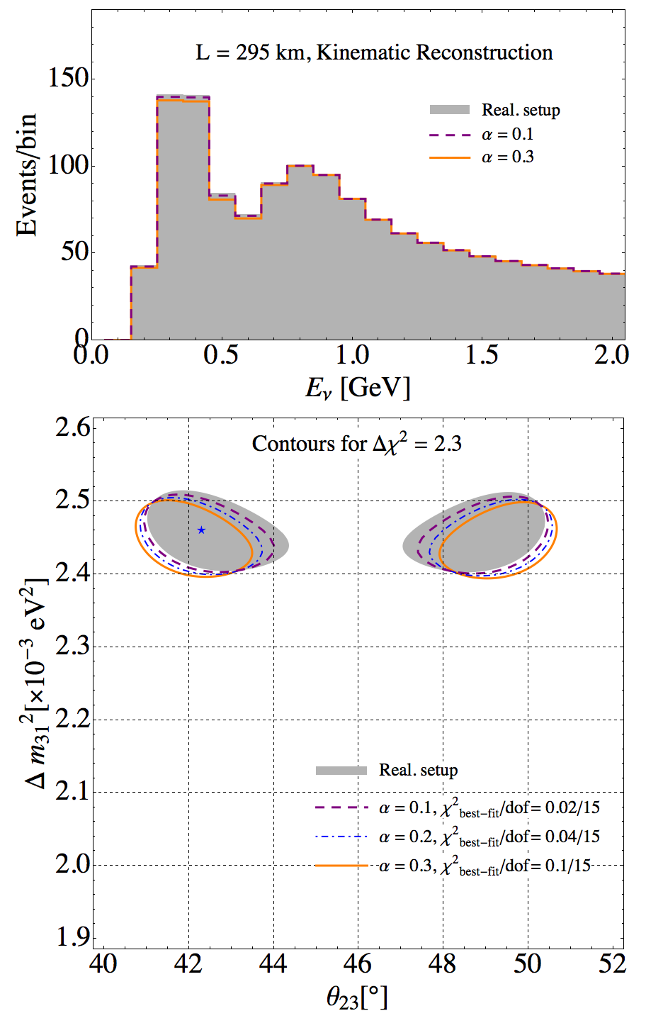
Figure 13: (color online). Same as in Fig. 11 but using the kinematic method to reconstruct the neutrino energy.

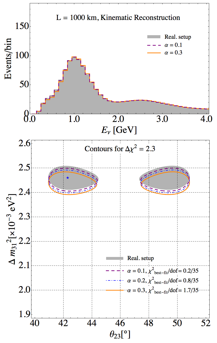
Figure 14: (color online). Same as in Fig. 11 but for the high-energy setup and the kinematic energy reconstruction.

As in Sec. VI.2, we calculate the true event distribution using the migration matrices accounting for realistic detection capabilities, while the fitted rates are obtained following Eq. (18), and the confidence regions satisfy Eq. (19).

Our results for the kinematic reconstruction method are shown in Figs. 13 and 14 for the LE and HE setups, respectively. In the case of the confidence regions represented by the shaded areas, the true and fitted rates are generated using the same set of migration matrices ($\alpha=0$), and, therefore, the best fit coincides with the true values. When the value of $\alpha$ increases, the confidence regions start to drift away from the shaded areas. This is a consequence of the fact that the shapes of the event distributions are generally different from that of the true rates, even for the same oscillation probability, and the best fit for the oscillation parameters no longer coincides with the true values.

However, it should be noted that for the kinematic reconstruction, the effect of the mismatch between the actual and assumed detector capabilities is much milder than for the calorimetric method. The confidence regions show a significant overlap, even for $\alpha=0.3$, corresponding to the detector performance substantially overestimated. The main reason for this is that the muon reconstruction is very precise in modern detectors, while for electrons and hadrons this is more difficult to achieve (see also Figs. 6 and 8). It should be noted, however, that in this study we assume that the muon track is fully contained in the detector, regardless of its energy. Should this assumption be relaxed, the muon momentum determination may be affected and, as a consequence, also the neutrino-energy reconstruction.

VII Summary

It has been realized for a while now that an accurate understanding of neutrino-nucleus scattering is an essential ingredient for neutrino-oscillation experiments employing accelerator beams. More recently, quantitative studies have tackled the relation between uncertainties in cross section modeling and the resulting physics sensitivities for oscillation measurements. For example, it was shown that for quasielastic events the energy reconstruction based exclusively on the kinematic observables of the outgoing lepton is susceptible to a large bias resulting from the underlying nuclear-interaction model ref:Pilar_PRD ; ref:Pilar_PRL . In this article, we fully rely on the nuclear model used for event generation, and have a critical look only at the impact of realistic detector effects.

From energy conservation, it is clear that a perfect calorimeter—i.e., a detector able to measure the total energy of all reaction products—would be free from any bias in energy reconstruction ref:Ulrich . In this article, we aim at quantifying how close to the perfect scenario the calorimetric energy reconstruction is, when finite energy resolutions, detection efficiencies, and thresholds are accounted for. In addition, we compare the role of realistic detection capabilities on the calorimetric and kinematic analysis. In the latter case, we use—although in a simplistic way—the information on that the charged lepton’s kinematics also for non-QE events.

We find that the kinematic reconstruction is very robust with respect to detector effects, largely because muons are the most precisely reconstructed particles in modern neutrino detectors. On the other hand, the actual performance of the calorimetric analysis clearly depends on the assumed detector performance. The employed detection capabilities are not meant to represent any existing detector, but are indicative of the general level of performance which can be expected. While to translate these result into a specific experiment a detailed study of detector response—beyond the scope of this work—would be required, many of the analysis techniques developed here should turn out to be very useful. Interestingly, we find that the kinematic reconstruction performs well even for pion-production events, but the independence of this observation from the underlying nuclear model is to be examined.

We limit our study to the $\nu_{\mu}$ disappearance channel since this can be effectively treated as a two-flavor oscillation. As a consequence, the effects of energy resolution and misreconstruction are directly related to the precision of the $\Delta m^{2}$ determination and a shift of the value of $\Delta m^{2}$, respectively. We use a phenomenological parametrization to interpolate between a perfect and realistic detector. This allows us to conclude that, overall, the detector response—in terms of efficiencies, resolutions, and thresholds for individual particles—has to be understood at a 10% level or better, to avoid a significant bias in the measurement of $\Delta m^{2}$. For the kinematic analysis, these requirements are much less stringent, but uncertainties of the nuclear model—not considered here—present a challenge, as shown previously in the literature.

In summary, while the calorimetric reconstruction may be less sensitive to the underlying nuclear model, it is strongly affected by detector effects, typically leading to energy underestimation. On the other hand, the kinematic method of neutrino energy reconstruction is much less challenging for the detector design, but it strongly relies on an accurate understanding of neutrino-nucleus interactions. One needs to keep in mind that the quantitative details of our conclusions may be specific to this work, owing to the underlying detector assumptions. However, their qualitative aspects can be expected to hold for a variety of experiments.

As a final remark, we observe that the results presented in this article are subject to nuclear-model uncertainties, likely to be largest for $2p2h$ processes. Their estimate is left to be quantified in our future studies.

- (1) K. Abe et al. (T2K Collaboration), Nucl. Instrum. Methods Phys. Res., Sect. A 659, 106 (2011).
- (2) A. A. Aguilar-Arévalo et al. (MiniBooNE Collaboration), Nucl. Instrum. Methods Phys. Res., Sect. A 599, 28 (2009).
- (3) M. Martini, M. Ericson, G. Chanfray, and J. Marteau, Phys. Rev. C 80, 065501 (2009).
- (4) D. G. Michael et al. (MINOS Collaboration), Nucl. Instrum. Methods Phys. Res., Sect. A 596, 190 (2008).
- (5) D. S. Ayres et al. (NOA Collaboration), Fermilab-Proposal-0929, arXiv:hep-ex/0503053.
- (6) C. Adams et al. (LBNE Collaboration), arXiv:1307.7335.
- (7) H. Gallagher, talk given at the INT Workshop “Neutrino-Nucleus Interactions for Current and Next Generation Neutrino Oscillation Experiments” (INT-13-54W), Seattle, USA, 3–13 December 2013; the slides and video available at http://www.int.washington.edu/talks/WorkShops/int_13_54W/.
- (8) Q. Wu et al. (NOMAD Collaboration), Phys. Lett. B660, 19 (2008).
- (9) V. V. Lyubushkin et al. (NOMAD Collaboration), Eur. Phys. J. C 63, 355 (2009).
- (10) A. A. Aguilar-Arévalo et al. (MiniBooNE Collaboration), Phys. Rev. D 81, 092005 (2010).
- (11) A. A. Aguilar-Arévalo et al. (MiniBooNE Collaboration), Phys. Rev. D 82, 092005 (2010).
- (12) A. A. Aguilar-Arévalo et al. (MiniBooNE Collaboration), Phys. Rev. D 83, 052007 (2011).
- (13) A. A. Aguilar-Arévalo et al. (MiniBooNE Collaboration), Phys. Rev. D 83, 052009 (2011).
- (14) Y. Nakajima et al. (SciBooNE Collaboration), Phys. Rev. D 83, 012005 (2011).
- (15) L. Fields et al. (MINERvA Collaboration), Phys. Rev. Lett. 111, 022501 (2013).
- (16) G. A. Fiorentini et al. (MINERvA Collaboration), Phys. Rev. Lett. 111, 022502 (2013).
- (17) K. Abe et al. (T2K Collaboration), Phys. Rev. D 87, 092003 (2013).
- (18) A. A. Aguilar-Arévalo et al. (MiniBooNE Collaboration), Phys. Rev. D 88, 032001 (2013).
- (19) K. Abe et al. (T2K Collaboration), Phys. Rev. D 90, 052010 (2014).
- (20) B. G. Tice et al. (MINERvA Collaboration), Phys. Rev. Lett. 112, 231801 (2014).
- (21) K. Abe et al. (T2K Collaboration), Phys. Rev. Lett. 113, 241803 (2014).
- (22) A. Higuera et al. (MINERvA Collaboration), Phys. Rev. Lett. 113, 261802 (2014).
- (23) A. A. Aguilar-Arévalo et al. (MiniBooNE Collaboration), Phys. Rev. D 91, 012004 (2015).
- (24) T. Walton et al. (MINERvA Collaboration), Phys. Rev. D 91, 071301(R) (2015).
- (25) K. Abe et al. (T2K Collaboration), Phys. Rev. D 91, 112002 (2015).
- (26) B. Eberly et al. (MINERvA Collaboration), arXiv:1406.6415.
- (27) K. Abe et al. (T2K Collaboration), arXiv:1411.6264.
- (28) T. Le et al. (MINERvA Collaboration), Phys. Lett. B749, 130 (2015).
- (29) C. Andreopoulos et al., Nucl. Instrum. Methods Phys. Res., Sect. A 614, 87 (2010).
- (30) C.-M. Jen, A. M. Ankowski, O. Benhar, A. P. Furmanski, L. N. Kalousis, and C. Mariani, Phys. Rev. D 90, 093004 (2014).
- (31) O. Benhar, A. Fabrocini, S. Fantoni, and I. Sick, Nucl. Phys. A579, 493 (1994).
- (32) D. G. Michael et al. (MINOS Collaboration), Phys. Rev. Lett. 97, 191801 (2006).
- (33) O. Benhar and D. Meloni, Phys. Rev. D 80, 073003 (2009).
- (34) M. H. Ahn et al. (K2K Collaboration), Phys. Rev. Lett. 90, 041801 (2003).
- (35) A. A. Aguilar-Arévalo et al. (MiniBooNE Collaboration), Phys. Rev. Lett. 100, 032301 (2008).
- (36) T. Leitner and U. Mosel, Phys. Rev. C 81, 064614 (2010).
- (37) M. Martini, M. Ericson, and G. Chanfray, Phys. Rev. D 85, 093012 (2012).
- (38) M. Martini, M. Ericson, and G. Chanfray, Phys. Rev. D 87, 013009 (2013).
- (39) O. Lalakulich, K. Gallmeister, and U. Mosel, Phys. Rev. C 86, 014614 (2012); Phys. Rev. C 90, 029902(E) (2014).
- (40) S. Dytman, in 12th International Workshop on Neutrino Factories, Superbeams, and Betabeams (NuFact10) (Mumbai, India, 2010), edited by B. S. Acharya, M. Goodman, and N. K. Mondal, AIP Conf. Proc. No. 1382 (AIP, New York, 2011), p. 156.
- (41) D. Rein and L. M. Sehgal, Ann. Phys. (N.Y.) 133, 79 (1981).
- (42) A. Bodek and U.-K. Yang, J. Phys. G 29, 1899 (2003).
- (43) A. Bodek, I. Park, and U.-K. Yang, Nucl. Phys. B, Proc. Suppl. 139, 113 (2005).
- (44) T. Yang, C. Andreopoulos, H. Gallagher, K. Hofmann, and P. Kehayias, Eur. Phys. J. C 63, 1 (2009).
- (45) Z. Koba, H.B. Nielsen, and P. Olesen, Nucl. Phys. B40, 317 (1972).
- (46) T. Sjöstrand, S. Mrenna, and P. Skands, J. High Energy Phys. 05 (2006) 026.
- (47) T. Katori, in Nuint12: The 8th International Workshop on Neutrino-Nucleus Interactions in the Few-GeV Region, edited by H. da Motta, J. G. Morfin, and M. Sakuda, AIP Conf. Proc. 1663, 030001 (2015).
- (48) J. W. Lightbody Jr. and J. S. O’Connell, Comput. Phys. 2, 57 (1988).
- (49) C. H. Llewellyn Smith, Phys. Rep. 3, 261 (1972).
- (50) A. Bodek and J. L. Ritchie, Phys. Rev. D 23, 1070 (1981).
- (51) O. Benhar, D. Day, and I. Sick, Rev. Mod. Phys. 80, 189 (2008).
- (52) O. Benhar, A. Fabrocini, and S. Fantoni, Nucl. Phys. A505, 267 (1989).
- (53) J. Mougey et al., Nucl. Phys. A262, 461 (1976).
- (54) D. Dutta et al., Phys. Rev. C 68, 064603 (2003).
- (55) A. M. Ankowski, O. Benhar, and M. Sakuda, Phys. Rev. D 91, 033005 (2015).
- (56) D. Rohe et al. (JLAB E97-006 Collaboration), Nucl. Phys. B, Proc. Suppl. 159, 152 (2006).
- (57) V. Barger et al., arXiv:0705.4396 [hep-ph].
- (58) S. Short, Ph.D. thesis, Imperial College London, 2013.
- (59) B. Eberly, in Nuint12: The 8th International Workshop on Neutrino-Nucleus Interactions in the Few-GeV Region, edited by H. da Motta, J. G. Morfin, and M. Sakuda, AIP Conf. Proc. 1663, 070006 (2015).
- (60) L. Aliaga et al. (MINERvA Collaboration), Nucl. Instrum. Methods Phys. Res., Sect. A 743, 130 (2014).
- (61) A. A. Aguilar-Arévalo et al. (MiniBooNE Collaboration), Phys. Rev. Lett. 98, 231801 (2007).
- (62) A. Stahl et al., CERN-SPSC-2012-021, SPSC-EOI-007. http://inspirehep.net/record/1194418/files/SPSC-EOI-007.pdf
- (63) H. Berns, H et al. (CAPTAIN Collaboration), arXiv:1309.1740.
- (64) Q. Liu, Phys. Procedia 61, 483 (2015).
- (65) For the migration matrices and the cross sections employed in our analysis see Ancillary Files accompanying this article. They are also available at http://chimera.roma1.infn.it/OMAR/Erica/.
- (66) S. K. Agarwalla, S. Prakash, S. K. Raut, and S. U. Sankar, JHEP 1212, 075 (2012) [arXiv:1208.3644 [hep-ph]].
- (67) S. K. Agarwalla, S. Prakash, and W. Wang, arXiv:1312.1477.
- (68) S. K. Agarwalla, T. Li and A. Rubbia, JHEP 1205, 154 (2012) [arXiv:1109.6526 [hep-ph]].
- (69) R. B. Patterson, Nucl. Phys. B, Proc. Suppl. 235-–236, 151 (2013).
- (70) P. Huber, M. Lindner, T. Schwetz, and W. Winter, JHEP 0911, 044 (2009) [arXiv:0907.1896 [hep-ph]].
- (71) H. Nunokawa, S. J. Parke, and R. Zukanovich Funchal, Phys. Rev. D 72, 013009 (2005).
- (72) G. L. Fogli and E. Lisi, Phys. Rev. D 54, 3667 (1996).
- (73) V. Barger, D. Marfatia, and K. Whisnant, Phys. Rev. D 65, 073023 (2002).
- (74) J. Burguet-Castell, M. B. Gavela, J. J. Gomez-Cadenas, P. Hernandez, and O. Mena, Nucl. Phys. B608, 301 (2001).
- (75) H. Minakata and H. Nunokawa, JHEP 0110, 001 (2001) [hep-ph/0108085].
- (76) A. Donini, D. Meloni, and S. Rigolin, JHEP 0406 (2004) 011 [hep-ph/0312072].
- (77) H. Minakata and S. J. Parke, Phys. Rev. D 87, 113005 (2013).
- (78) P. Coloma, H. Minakata, and S. J. Parke, Phys. Rev. D 90, 093003 (2014).
- (79) A. M. Ankowski, Proc. Sci. NUFACT2014 (2015) 004.
- (80) P. Coloma, E. Fernandez-Martinez, and L. Labarga, JHEP 1211, 069 (2012) [arXiv:1206.0475 [hep-ph]].
- (81) P. Coloma, T. Li, and S. Pascoli, arXiv:1206.4038 [hep-ph].
- (82) P. Huber and J. Kopp, JHEP 1103, 013 (2011) [JHEP 1105, 024 (2011)] [arXiv:1010.3706 [hep-ph]].
- (83) T. Akiri et al. (LBNE Collaboration), arXiv:1110.6249.
- (84) J. A. Formaggio and G. P. Zeller, Rev. Mod. Phys. 84, 1307 (2012).
- (85) P. Coloma and P. Huber, Phys. Rev. Lett. 111, 221802 (2013).
- (86) P. Coloma, P. Huber, C.-M. Jen, and C. Mariani, Phys. Rev. D 89, 073015 (2014).
- (87) P. Coloma, P. Huber, J. Kopp, and W. Winter, Phys.Rev. D 87, 033004 (2013).
- (88) P. Huber, M. Lindner, and W. Winter, Comput. Phys. Commun. 167, 195 (2005).
- (89) P. Huber, J. Kopp, and M. Lindner, Comput. Phys. Commun. 177, 432 (2007).
- (90) A. M. Dziewonski and D. L. Anderson, Phys. Earth Planet. Inter. 25, 297 (1981).
- (91) R. Gran et al. (K2K Collaboration), Phys. Rev. D 74, 052002 (2006).
- (92) S. K. Agarwalla et al. (LAGUNA-LBNO Collaboration), arXiv:1412.0804.
- (93) D. Beavis et al. (E889 Collaboration), Physics Design Report, BNL 52459, 1995; J.-M. Levy, arXiv:1005.0574.
- (94) P. Huber, M. Lindner, T. Schwetz, and W. Winter, J. High Energy Phys. 11 (2009) 044.
- (95) K. Abe et al. (T2K Collaboration), Phys. Rev. D 87, 012001 (2013).
- (96) A. Longhin, arXiv:1206.4294.
- (97) D. Angus et al. (LAGUNA Collaboration), arXiv:1001.0077.
- (98) U. Mosel, arXiv:1504.08204.