A new hydrodynamics code for Type Ia Supernovae

Abstract

A two-dimensional hydrodynamics code for Type Ia supernovae (SNIa) simulations is presented. The code includes a fifth-order shock-capturing scheme WENO, detailed nuclear reaction network, flame-capturing scheme and sub-grid turbulence. For post-processing we have developed a tracer particle scheme to record the thermodynamical history of the fluid elements. We also present a one-dimensional radiative transfer code for computing observational signals. The code solves the Lagrangian hydrodynamics and moment-integrated radiative transfer equations. A local ionization scheme and composition dependent opacity are included. Various verification tests are presented, including standard benchmark tests in one and two dimensions. SNIa models using the pure turbulent deflagration model and the delayed-detonation transition model are studied. The results are consistent with those in the literature. We compute the detailed chemical evolution using the tracer particles’ histories, and we construct corresponding bolometric light curves from the hydrodynamics results. We also use a Graphics Processing Unit (GPU) to speed up the computation of some highly repetitive subroutines. We achieve an acceleration of 50 times for some subroutines and a factor of 6 in the global run time.

1 Introduction

1.1 Chandrasekhar Mass Explosion Model

A Type Ia supernova (SNIa) is the explosion of a carbon-oxygen white dwarf (WD) due to thermonuclear runaway of carbon burning. It is believed to be a standard candle due to its observed explosion homogeneity (Branch & Tammann, 1992) and the luminosity-width relation (Phillips et al., 1987). Also, in numerical modeling, the standard Chandrasekhar mass WD is regarded as the progenitor of an SNIa. These properties lead to wide applications of SNIa as a cosmological ruler for determining the Hubble parameters (Leibundgut & Pinto, 1992), and the discovery of dark energy (Riess et al., 1998; Perlmutter et al., 1999).

In the last few decades, several explosion mechanisms have been proposed, starting from the pure detonation model of Chandrasekhar mass WD proposed in Arnett (1969). Despite its ability in unbinding the whole star, the over-production of iron-peaked elements and the absence of intermediate mass elements (IME) make this scheme implausible (Nomoto & Sugimoto, 1977). Later, the sub-sonic pure deflagration model is proposed, which aims at providing sufficient time for electron capture in the laminar flame stage (Nomoto et al., 1976) and production of IME. The weakness of pure detonation model is resolved but the deflagration wave is too slow to unbind the WD. The flame is quenched before consuming the whole WD, which leaves a large amount of unburnt material (fuel) (Nomoto et al., 1976). In view of this dilemma, several flame acceleration schemes or transition schemes are proposed. Popular models include the delayed-detonation transition model (DDT), the pure turbulent deflagration (PTD) model and the gravitationally confined detonation (GCD) model.

The DDT model is first suggested by Khokhlov (see for example Khokhlov (1989, 1991a)). It is believed that the eddies around the flame front may provide the required environment, which seeds the detonation spot by the Zel’dovich gradient mechanism (Khokhlov, 1991b). It has a counterpart in the shocktube experiment. The model has been found satisfactory because of the sufficient production of IME, absence of remnant and consumption of fuel around the core (Khokhlov, 1989; Gamezo et al., 2004, 2005). However, whether the first detonation spot can be seeded is still an open question. It is believed that the velocity fluctuations are adequate for triggering the detonation (Khokhlov et al., 1995). On the other hand, several turbulent flame simulations (see for example Niemeyer (1999), Imshenik et al. (1999), and Lisewski et al. (2000)) have shown that the developed velocity fluctuations are far below the required level. Also, the detonation front is found to be unstable when encountering obstacles (Maier & Niemeyer, 2006). This makes the robustness of this mechanism in doubt.

The PTD model assumes that the the fluid is highly turbulent in view of the high Reynolds number (Niemeyer & Hillebrandt, 1995b). Local velocity fluctuations are important for the flame evolution because the flame is constantly stretched and perturbed by the fluid motion, which enlarges the local burning surface (Khokhlov, 1994). This increases the fuel consumption rate and hence makes the flame propagate faster, compared with a laminar flame under the same condition (Timmes, 1992). Two models are commonly considered in turbulent flame modeling. The first model is proposed in (Damkoehler, 1939). It is observed in Bunsen flame experiments that the turbulent flame propagation speed $v_{{\rm turb}}$ varies with local turbulence fluctuations $\tilde{v}$: $v_{{\rm turb}}=\tilde{v}$ (Niemeyer & Hillebrandt, 1995a). The second model is obtained from a theoretical analysis (Pocheau, 1994). It is found that $v_{{\rm turb}}=v_{{\rm lam}}\sqrt{1+C(\tilde{v}/v_{{\rm lam}})^{2}}$ with $v_{{\rm lam}}$ being the laminar flame speed. The applications of turbulent flame in the SNIa explosion scenario are first proposed in Niemeyer & Hillebrandt (1995a), based on the sub-grid turbulence model reported in Clement (1993). The model has been found successful in providing a healthy explosion in two-dimensional (Reinecke et al., 2002a) and three-dimensional simulations (Reinecke et al., 2002b; Roepke & Hillebrandt, 2005; Roepke, 2005). However, several drawbacks have been found in detailed three dimensional studies. They include the presence of low-velocity fuels (carbon and oxygen) in the ejecta and underproduction of IME (Roepke et al., 2007).

The GCD model, also known as the Deflagration Failed Detonation (DFD) model (Plewa & Kasen, 2007; Kasen & Plewa, 2007), is similar to the DDT model, which starts from the deflagration phase. But the burning is weak so that the star remains bound. The hot and burnt material causes the WD to expand, floating the hot flame by buoyancy to the surface. After then, a large amount of fuel remains unburnt. The flame propagates throughout the WD by a surface flow (Jorden et al., 2008). The flow finally merges at one point, usually at the point opposite to the breakout location (Meakin et al., 2009). The converging flow heats up the cold and low-density fuel, pushing it deep inside the star. Once the squeezed fuel becomes the hot spot for detonation as its density exceeds the threshold, a detonation front forms, which burns the remaining stellar material and unbinds the whole WD (Jorden et al., 2012). The qualitative difference between DDT model and GCD model is that, in the former, the detonation starts from the inside of the WD and sweeps outward, while it is the opposite in the latter.

Recent developments of hydrodynamics models have considered extensively all three models. In Long et al. (2014), three-dimensional PTD models are studied. In Seitenzahl et al. (2012), the DDT model is shown to be able to explain certain SNIa observation data. In Blondin et al. (2011) and Blondin et al. (2012), DDT models in one-dimension and two-dimension are studied with their synthetic spectra and light curves. Such fine details provide a mean to constrain the explosion model (Dessart et al., 2013).

1.2 Radiative Transfer

The modeling of post-explosion light curve and spectrum are crucial for discriminating the validity of an explosion mechanism. The governing physics of SNIa light curves are believed to be the decay of synthesized ⁵⁶Ni into ⁵⁶Co in early time, and decay of ⁵⁶Co into ⁵⁶Fe in late time (Colgate & White, 1969). Simplified models, including those with diffusion approximation (Colgate et al., 1980), or analytic models assuming a fireball undergoing homologous expansion (Arnett, 1982), can already capture primary features of SNIa light curves and match a number of observed SNIa.

Despite that the light curves are well fitted by these models, in order to understand the variety of SNIa observations, as well as their relations with explosion models, detailed radiative transfer for both bolometric and multiple wavebands are important (Zhang & Sutherland, 1994). The actual problem of radiative transfer can be highly nontrivial due to its interactions with hydrodyanmics, the presence of millions to billions of atomic transition lines, ionization and excitation of atoms, and the differential-integral structure of the radiative transfer equations. These features have been studied in details in the last few decades. Physics and numerical factors, such as the effects of line blanketing (Hillier, 1990; Hillier & Miller, 1998), consistent boundary conditions (Sauer et al., 2006), treatment in opacities (Hoeflich et al., 1993), acceleration techniques (Hillier, 1990; Lucy, 2001) and so on have been studied extensively. A number of numerical codes for solving this problem have been under constant development in the past few decades (see STELLA (Blinnikov et al., 2008; Blinnikov & Sorokina, 2000; Blinnikov et al., 2006), ARTIS (Lucy, 2005; Sim, 2007; Kromer & Sim, 2009), SEDONA (Kasen, 2006) and PHOENIX (Hauschildt & Baron, 2010; Seelmann et al., 2010; Hauschildt & Baron, 2011) for the instrument papers and realizations).

Due to the stringent demand in computational resource for calculating radiative transfer, in previous studies, the explosion phase and its observational consequences are usually modeled separately (Nomoto et al., 1986; Zhang & Sutherland, 1994; Hoeflich et al., 1995; Nugent et al., 1997), where the radiative transfer part makes use of the hydrodyanmics results from some benchmark runs. Recent development of computational power allows the spectral synthesis to be coupled in the hydrodynamics to form a pipeline following the explosion and homologous expansion phases. Different explosion mechanisms have been studied with fine details, such as the PTD model (Fink et al., 2014; Long et al., 2014), DDT model (Blondin et al., 2011; Seitenzahl et al., 2012) and GCD model (Plewa & Kasen, 2007; Kasen & Plewa, 2007).

1.3 Flame Capturing Scheme

The flame capturing scheme is a technique of describing discontinuities with details in sub-grid scales. Such discontinuities can be in forms of fluid type, composition or characters. In SNIa simulations, it is essential because the typical width of deflagration waves is in the order of centimeters or even smaller. Also, their propagation speed is much slower than the fluid speed of sound. Therefore, within one time step under the Courant-Fredrich-Lewy condition, only a partial amount of a fluid element in a grid is burnt and so it is important to determine the ash-fuel interface in partially burnt grids.

To account for such discontinuities, three types of interface tracking algorithms are commonly used. The first one is the level-set method (Osher & Sethian, 1988). This method suggests that the discontinuity can be described by the zero contour of a scalar function, which is interpreted as the distance function. This method has advantages in its easy implementation and direct coupling with hydrodynamics. Also, the scheme can be generalized directly to arbitrary dimensions. The topological changes are handled naturally without the need of extra spotting mechanism (Sethian, 2001). However, it is also known to have poor volume conservation (Rider & Kothe, 1995). The distance function requires reinitialization at each iteration step in order to preserve the distance function validity (Sussman et al., 1994). This scheme in SNIa is first proposed by Reinecke et al. (1999), and applications are found in Reinecke et al. (1999, 2002a, 2002b).

Another algorithm is the point-set method (Glimm et al., 1981; Glimm & McBryan, 1985; Glimm et al., 1988). The flame front is described as a line in a two-dimensional simulation or a surface in a three-dimensional simulation, by a linked set of massless particles which are advected along the streamline of fluid flow, and they only reveal the position of the interface without affecting the hydrodynamics properties of the fluid. This method receives wide applications in other fields, such as the study of bubbles (Youngren & Acrivos, 1976). It has a huge advantage that the interface properties are exactly modeled, such that their geometric properties can be obtained in a straightforward manner (Tryggvason et al., 2001). However, it has two major shortcomings. First, it requires special attention in topological changes, namely surface splitting and merging (Glimm et al., 1988). Also, the extension of the point-set method to three-dimensional simulations is non-trivial, because the surface is no longer represented by a line segment (Glimm et al., 1999). For example of application, see Zhang (2009) for a laminar deflagration model. It is shown that, with sufficient fine details, the laminar flame can bring a successful explosion without the need of any flame acceleration scheme.

The third mechanism which is commonly found in the literature is the volume of fluid method (Hirt & Nichols, 1981). This method is similar to the level-set method, which introduces an extra scalar field that represents the volume fraction of a specific fluid. This model is also regarded as the advection-diffusion-reaction equation (Calder et al., 2007; Townsley et al., 2007). The method is known for its exact conservation of mass (Scadovelli & Zaleski, 1999). However, the implicit nature of geometric quantities becomes its disadvantage. The geometry of the flame, which is important in reconstructing the thermodynamics of partially burnt grids, is dependent of the reconstruction scheme (Rudman, 1997). In SNIa context, the algorithm is pioneered in simulations presented in Khokhlov (1993). The FLASH code has adopted this algorithm as the default flame capturing scheme; see for example (Calder et al., 2007).

1.4 Sub-grid Turbulence

The fluid motion can be turbulent because of the high Reynolds number. The flame surface is known to be unstable subject to hydrodynamic instabilities related to turbulence. The eddies stretch and perturb the flame front, which increase its effective burning area and enhance burning rate (Timmes, 1992), when compared with laminar flame at the same density. Similar to the difficulties in resolving the flame interface, the eddies have sizes down to the Kolmogorov’s scale ($\sim$ cm) (Woosley et al., 2009), and therefore a direct numerical modeling of these eddies is not yet feasible. Instead, sub-grid turbulence is employed to mimic the small-scale eddies by scaling kinematics from large scales.

Various implementations of sub-grid turbulence models are proposed. They can be classified mainly into the one-equation model, two-equation model and Reynolds stress model. In all these models, the production/dissipation rates are closed by direct numerical simulations, statistical closure or dynamical modeling.

The one-equation model, first proposed by Smagorinsky (1963), introduces the turbulence kinetic energy $q$. It first appears in the SNIa simulation in Niemeyer & Hillebrandt (1995a), which relies on a statistical model based on Kolmogorov’s scaling (Clement, 1993). The model gives breakthroughs by providing a healthy explosion, as shown in Reinecke et al. (2002a). However, it is argued that the dissipation might not be following Kolmogorov’s one instantaneously (Schmidt et al., 2006). The model is later extended in Schmidt et al. (2005), which generalizes the eddy production or dissipation terms dynamically.

The two-equation model, first proposed in Launder & Spalding (1974), introduces two extra quantities, which model the decay of eddies by an extra dissipation term $\epsilon$ ($q-\epsilon$ model) or a vorticity term $\omega$ ($q-\omega$ model). Both models aim at describing the dissipation of eddies. However, the original equations do not guarantee the positivity of $q$ and $\epsilon$ (non-realizable). We refer the reader to Shih et al. (1994) for modifications of the equations that can guarantee the realizability condition. Unlike the one-equation model, this model is not applied in common SNIa simulations.

The Reynolds stress model provides algebraic closure to the sub-grid velocity correlations (Shih et al., 1995). However, not all the variables can be closed by direct numerical simulations due to the larger number of coefficients. A similar problem can already be found in some extensions of the two-equation model. For instance, in the three-equation model, an ad hoc timescale is needed in order to close the equation set (Yoshizawa et al., 2012).

1.5 Motivation and Structure

In SNIa literature several codes are commonly used for studying the explosion phase. The first one is LEAFS, which is known as PROMETHEUS in earlier publications (see for example (Reinecke et al., 1999)). This code makes use of the piecewise-parabolic method (PPM) (Collela & Woodward, 1984) with moving meshes that follow the WD expansion (see Roepke & Hillebrandt (2005); Roepke (2005) for the development and early applications). The code models the turbulent nuclear flame using a sub-grid turbulence algorithm with the level-set method as flame-tracking scheme. This code has been used in large-scale massively parallel runs in PTD (Fink et al., 2014) and DDT models (Seitenzahl et al., 2012). Another hydrodynamics code is the FLASH code (Fryxell et al., 2000). This code is embedded with adaptive-mesh refinement such that the flame structure can be traced with fine details. Recently, FLASH has been developed into a part of a pipeline in SNIa numerical tool in constructing, analyzing and comparing numerical data with observations (Long et al., 2014). The code uses the advection-diffusion-reaction scheme in describing the ash distribution and flame geometry but without sub-grid turbulence. Recent large-scale computations in the PTD models (Long et al., 2014) and GCD models (Jorden et al., 2012) have used this open-source code. We compare our code with LEAFS and FLASH in Table 1.

There are two motivations for us to build our own hydrodynamics code. First, at the time when the code was being developed, there was not yet a published SNIa code which makes use of a 5th order scheme in spatial discretization. Second, we shall apply the hydrodynamics code to various astrophysical contexts. One of our work in progress is to study the effects of dark matter on SNIa explosions (Leung et al., 2015b). By building our own code, it is easier for us to implement and analyze any additional physics component in SNIa simulations.

Table 1: Comparison of the numerical components and structure of our code with other commonly used hydrodynamics codes.

Scheme	Our code	LEAFS (PROMETHEUS)	FLASH
Spatial discretization	WENO 5th order	PPM	PPM/WENO
Accuracy	$5^{{\rm th}}$ order	$3^{{\rm rd}}$ order	$3^{{\rm rd}}-5^{{\rm th}}$ order
Time discretization	Runge-Kutta 5-Step	Directional splitting	Directional splitting
Accuracy	$3^{{\rm rd}}$ order	$2^{{\rm nd}}$ order	$2^{{\rm nd}}$ order
Adaptive Mesh Refinement	No	No	Yes
Dimensions	1-2	1-3	1-3
Flame capturing scheme	Level-set ($default$)	Level-set	ADR
	Point-set
Sub-grid turbulence	Yes	Yes	No
Number of online isotopes	19	5	3
Hardware acceleration	GPU	Multi-processors	Multi-processors

In this article, we report numerical tests of our hydrodynamics code and comparisons with other benchmark tests reported in the literature. In Section 2, we describe the hydrodynamics equations and the numerical techniques that we implement in our code. In Section 3 we describe the input physics for modeling SNIa. We also introduce the radiative transfer code by describing its numerical implementation. Then in Section 4 we outline the post-processing tools we have used in extracting observables from the hydrodynamics results, including the tracer particle method and the one-dimensional moment-integrated radiative transfer code. In Section 5, we report our results. We describe the configurations and results of some benchmark one- and two- dimensional tests. We also show two test runs using the PTD and DDT models, and we compare our results with some similar runs in the literature. In Section 6 we describe the results after post-processing, including the detailed nucleosynthesis yields, bolometric light curves and the synthetic spectra. In Section 7, we summarize and briefly outline our future plans.

2 Methods

2.1 Hydrodynamics

We have developed a two-dimensional Eulerian hydrodynamical code in cylindrical coordinates to model SNIa. The equations include

$$\frac{\partial\rho}{\partial t}+\frac{\partial\rho v_{r}}{\partial r}+\frac{\partial\rho v_{z}}{\partial z}=-\frac{\rho v_{r}}{r},$$ (1)

$$\frac{\partial\rho v_{r}}{\partial t}+\frac{\partial(\rho v_{r}^{2}+p)}{\partial r}+\frac{\partial\rho v_{r}v_{z}}{\partial z}=-\frac{\rho v_{r}^{2}}{r}-\rho\frac{\partial\Phi}{\partial r},$$ (2)

$$\frac{\partial\rho v_{z}}{\partial t}+\frac{\partial\rho v_{r}v_{z}}{\partial r}+\frac{\partial(\rho v_{z}^{2}+p)}{\partial z}=-\frac{\rho v_{r}v_{z}}{r}-\rho\frac{\partial\Phi}{\partial z},$$ (3)

$$\frac{\partial\tau}{\partial t}+\frac{\partial(\tau+p)v_{r}}{\partial r}+\frac{\partial(\tau+p)v_{z}}{\partial z}=$$

$$-\frac{(\tau+p)v_{r}}{r}-\rho\left(v_{r}\frac{\partial\Phi}{\partial r}+v_{z}\frac{\partial\Phi}{\partial z}\right)+\dot{Q}.$$ (4)

In the above equations, $(r,z)$ are the distances from the polar axis and the symmetry plane. $\rho$, $v_{r}$, $v_{z}$, $p$ and $\tau$ are the mass density, velocities in $r$ and $z$ directions, pressure and total energy density of the fluid. The total energy density includes both the thermal and kinetic parts $\tau=\rho\epsilon+\frac{1}{2}\rho v^{2}$, where $\epsilon$ is the specific internal energy. $\Phi$, the gravitational potential, satisfies the Poisson Equation $\nabla^{2}\Phi=4\pi G\rho$. $\dot{Q}=\dot{Q}_{{\rm nuc}}-\dot{Q}_{\nu}-\dot{Q}_{{\rm turb}}$ is the heat source and loss from nuclear fusion, neutrino emission and sub-grid turbulence. Note that we deliberately arrange the Euler equations into this conservative form in order to couple them with the Weighted Essential Non-Oscillatory scheme (WENO) directly. The terms on the right hand side are regarded as source terms.

We use a high-resolution shock-capturing scheme, WENO (Barth & Deconinck, 1999), for spatial discretization. This is a fifth-order scheme, which processes piecewise smooth functions with discontinuities in order to simulate the flux across grid cells with high precision, while avoiding spurious oscillations around the shock. In the code, we use a finite-difference formulation of the WENO scheme while the hydro quantities in the simulations, such as $\rho$, $v$, $\epsilon$ and so on, represent the averaged values of the actual profiles across the Eulerian grid. For the construction of numerical fluxes, we use the WENO-Roe scheme (Jiang & Shu, 1996). First we separate the hydro flux into a positive flux and a negative flux by a global Lax-Friedrichs splitting. Then we apply the WENO reconstruction on the two fluxes by an upwinding scheme. The numerical flux is obtained by summing the reconstructed positive and negative fluxes.

For the discretization in time, we use the five-stage, third-order, non-strong-stability-preserving explicit Runge Kutta scheme (Barth & Deconinck, 1999). Note that in the original prescription the three-stage, third-order, strong-stability-preserving explicit Runge-Kutta scheme is suggested. However, comparison of these two schemes shows that the latter one has no stability advantage and is less efficient (Wang & Spiteri, 2007). Therefore, we adopt the new time-discretization scheme.

The gravitational potential $\Phi$ is obtained by solving the Poission equation $\nabla^{2}\Phi=4\pi G\rho$. We use the successive over-relaxation method with the Gauss-Seidel method to solve the Poisson equation in cylindrical coordinates. The iteration is stopped by default when the relative changes of all grids reach below 10^-8. The inner boundaries are assumed to be reflecting and the outer boundaries are fixed by using the Roche approximation, which is given by $\Phi(r,z)=-GM/\sqrt{r^{2}+z^{2}}$. We remark that the Roche approximation assumes point-like mass everywhere, but in general higher multipole terms are needed. In our case, since the outer boundaries lie about a few times of the initial stellar radius away from the center of the star, the higher multipoles’ contributions are negligible. We find that the quadruple term gives a less than $1\%$ correction to the monopole term throughout the simulations.

2.2 Level-set method

We use the level-set method to trace the geometry of the flame front. This method is widely applied to other areas which require a detailed description of surfaces. It has been applied in SNIa modeling as prescribed in details in Reinecke et al. (1999). For the sake of completeness, we outline the governing equations and its procedure.

The level-set method introduces an extra scalar field $S$ imposed on an Eulerian grid, which satisfies $|\nabla S|=1$. The flame front is defined by the zero-contour of the field. We also define grids with positive (negative) values of $S$ to be full of ash (fuel). Geometrically speaking, the value is the minimum separation of a given point to the zero-contour surface.

The flame front propagates by both fluid advection and flame burning, which can be written as

$$\frac{\partial S}{\partial t}=-(\vec{v}+\vec{v}_{{\rm flame}})\cdot\nabla S.$$ (5)

$\vec{v}$ is the velocity of the fluid, governed by the compressible Euler equations. $\vec{v}_{{\rm flame}}$ is the effective flame propagation speed obtained from the nuclear reactions described in Sec. 3.2, which points towards the outward normal direction of the flame surface. For the dependence on density or composition of the flame speed, see in Appendix A their derivations and analytic fits.

With the evolution equations, we may simultaneously evolve the flame front coupled with the hydrodynamics. Note that in our simulations, the scalar field is defined on the corners of a grid, such that the position of flame front on the grid boundary can be found exactly.

In updating the scalar field, we make use of operator splitting to deal with the contributions from fluid advection and flame propagation. The latter part can be done with a common high-order advection scheme such as the piecewise-parabolic method (PPM) (Collela & Woodward, 1984) or the WENO scheme, such that the advection may preserve the area (volume) of the flame. Naturally, we use the WENO scheme as we have used to solve the hydrodynamics. After each update in $S$, we need to do a reinitialization (or redistancing) such that the scalar field $S$ can maintain the distance property $|\nabla S|=1$. We describe the procedure below.

First, we enumerate all positions where the flame front cut the grid, by finding all neighboring pairs of the scalar field where its values are of opposite signs. The position of the flame front is obtained by linear interpolation. Then the distances of all grid points to the flame front positions are compared, and the smallest one is chosen as the new value of $S$.

Note that this procedure preserves the distance property of $S$, but it perturbs the current flame position as well. Therefore, a smooth transition from its original value to the corrected value is used. When the grid is far away from the flame front, the distance value is used, otherwise the original value is kept. Mathematically, for a given scalar field $S_{{\rm old}(i,j)}$ with a minimum flame distance $d_{(i,j)}$, we have

$$S_{{\rm new}(i,j)}=H(d_{(i,j)})S_{{\rm old}(i,j)}+(1-H(d_{(i,j)}))d_{(i,j)},$$ (6)

where $H(d)$ is a smooth function satisfying $H(0)=1$ and $H(\infty)=0$. In our case, we follow the choice of Reinecke et al. (1999) that

$$H(d)=\frac{1-{\rm tanh}\frac{d-d_{0}}{\Delta/3}}{1-{\rm tanh}\frac{-d_{0}}{\Delta/3}},$$ (7)

with $d_{0}=3\Delta$, $\Delta$ being the grid size in our simulations. This formula implies that the values of $S$ on the three closest neighboring grids around the flame front are unchanged.

As we have mentioned, the level-set method is not the only flame-capturing method. We have also developed the point-set method in order to compare their performances. See Appendix C for the details and numerical results.

2.3 GPU accelerations

In view of a large number of subroutines involved in each time step, we share parts of the computation with a graphics processing unit (GPU). By allowing the computations to be simultaneously done by more than thousands of threads, the total computation time can be drastically reduced, especially when the job requires repetitive but similar operations.

One major difference in CPU coding and GPU coding is the lack of static memory in GPU. Such a feature has made the use of GPU in typical hydrodynamics simulations unfavorable because the static memory provides convenient access to data, including the hydrodynamics variables and chemical composition, without the need of passing a large amount of variables among subroutines. Furthermore, such data migration, if not handled carefully, can take up even more time than using CPU solely. Nevertheless, the use of GPU can be advantageous when applied to subroutines that do not have the above undesirable properties.

In Table LABEL:table:TestGPU we tabulate the subroutines being processed by an NVIDIA GT Titan Black GPU and their running time, compared with an Intel I7 quad-core CPU. They include the Poisson solver, reinitialization procedure in the level-set method, WENO scheme and spatial discretization in other subroutines.

In general, two classes of time reduction can be found. For subroutines with pure matrix operations or repetitive procedures, such as the Poisson solver or the reinitialization scheme, a factor of 20-40 reduction can be obtained. For subroutines with heavy data transfer or significant amount of logical operations, such as the WENO scheme or the spatial discretization (which includes flux limiter), the time reduction is less significant, about a factor of 2 or less. Overall, there is a factor of 6 reduction in run time by using both CPU and GPU, compared with runs which make use of CPU only.

Table 2: A sample run of the code and a comparison of running time of subroutines with GPU version in one step. Subroutine time lapses are in unit of seconds and the full run is in units of hours. CPU: Intel I7, GPU: NVIDIA Titan Black.

subroutines	run time	run time
	CPU only	CPU + GPU
WENO scheme (s)	3.45	2.06
Poisson solver (s)	468.42	12.07
Reinitialization (s)	20.18	1.20
Spatial discretization (s)	1.08	1.10
One full run (hour)	199.66	29.78

3 Input physics

3.1 Equation of states

To close the equation set, we use the open-source Helmholtz equation of state (EOS) reported in Timmes & Swesty (1999) and Timmes et al. (2000). The EOS describes the equilibrium thermodynamical properties of a gas, which includes 1. electrons in the form of ideal gas with arbitrarily degenerate and relativistic levels, 2. ions in the form of classical ideal gas, 3. photons in Planck distribution, and 4. contributions from electron-positron pairs. The subroutine takes input of $\rho$, temperature $T$, mean atomic mass $\bar{A}$, mean atomic number $\bar{Z}$ and gives other thermodynamical quantities, including $p$, $\epsilon$, adiabatic index $\gamma$ and so on, together with their derivatives with respect to each input parameter.

3.2 Nuclear Reaction Network

To calculate the nuclear reaction heat production $\dot{Q}_{{\rm nuc}}$, we use the 19-isotope nuclear reaction network subroutine reported in F. X & Arnett (1999). The isotopes include ¹H, ³He, ⁴He, ¹²C, ¹⁴N, ¹⁶O, ²⁰Ne, ²⁴Mg, ²⁸Si, ³²S, ³⁶Ar, ⁴⁰Ca, ⁴⁴T, ⁴⁸Cr, ⁵²Fe, ⁵⁴Fe, ⁵⁶Ni, neutron and proton. The fusion network includes series of reactions from hydrogen burning up to silicon burning. Both $(\alpha,\gamma)$ and $(\alpha,p)(p,\gamma)$ reactions are included. Other isotopes, including ²⁷Al, ³¹P, ³⁵Cl and so on are included implicitly. Certain isotopes are less important here, for example, ¹H, ³He and ¹⁴N. They are involved in hydrogen burning or CNO-cycle, which are not crucial in SNIa. On the other hand, isotopes along the $\alpha$-particle chain are important for the exothermic processes in the explosions, as most energy is released by these processes, and the amount of ⁵⁶Ni is important for observations.

We do not couple the nuclear fusion subroutine directly in the code except at low density for two reasons. First, the deflagration and detonation wave fronts at high density have widths much thinner than the numerical grid size, and so only a fractional change occurs in the grids which are partially burnt in each time step. The energy release and isotope variations will be over-estimated if the whole cell is considered. Hence, the energy release relies on the fractional changes of area (volume) being consumed by the deflagration and detonation wave front, which depends strongly on the local density, but weakly on the local temperature. On the other hand, at low density, the deflagration and detonation wave can have a width comparable with simulation grid size. Then computing the nuclear reaction yields with data from the whole cell is acceptable. Second, the accuracy cannot be much improved unless the isotope transport of the burning grids are well described. But an exact reconstruction is time-consuming and sensitive to the numerical accuracy. As shown in Reinecke et al. (1999), an exact reconstruction is difficult for grids with large numerical errors. As a result, we choose the less accurate scheme by using tables of reaction products and energy release as functions of the input density. We describe the construction method and results in Appendix A and Appendix B.

3.3 Sub-grid turbulence

The use of the Euler equations is a good approximation when the fluid viscosity is small. This is true for the case of a WD. In a WD the fluid has a typical Reynolds number $R_{e}\sim 10^{14}$. This gives a dissipation range $\eta$ related to the integral range $L$ by the Reynolds number

$$L=\eta R_{e}^{3/4}.$$ (8)

Therefore, the dissipation range is about $10^{-3}$ cm, and the scales in which turbulence needs to be directly modeled are far smaller than the simulation grid size $\Delta\approx 10^{6}$ cm. In this range $\eta<\Delta<L$, called the inertial range, the hydrodynamics is dominated by the inertial term in the Navier-Stoke Equation and the turbulent dissipation is independent of small-scale viscosity. This allows us to treat the fluid as an ideal fluid, and take the effects of unresolved turbulence statistically. In particular, the turbulent velocity satisfies the Kolmogorov’s scaling law, which suggests that the local velocity fluctuations $\tilde{v}(l)$ are related to the local length scale $l$ by

$$\tilde{v}(l)=\tilde{v}(L)\left(\frac{l}{L}\right)^{1/3},$$ (9)

and there is a constant energy transfer rate from large to small scales.

The sub-grid turbulence model is based on the above properties as described in Clement (1993). This model is originally used to resolve the problem of frozen flow as commonly found in simulations of astrophysical convection. Such flow consists of unphysically large scale flow in opposite directions within neighbouring cells. Note that this result is also a solution of the Euler equations. It appears because the simulation fails to recognize that such large velocity gradient can actually result in sub-grid turbulence, which dissipates the excess velocity gradient into thermal energy by its kinematic viscosity. In practice, the effects of sub-grid turbulence are included as a heat source $\dot{Q}_{{\rm turb}}$

$$\dot{Q}_{{\rm turb}}=-A\rho q\nabla\cdot v+\Sigma_{ij}\frac{\partial v_{i}}{\partial x_{j}}-\rho\epsilon_{dis}+C_{{\rm Arch}}\rho g_{{\rm eff}},$$ (10)

where

$$\Sigma_{ij}=\rho\nu_{{\rm turb}}\left(\frac{\partial v_{i}}{\partial x_{j}}+\frac{\partial v_{j}}{\partial x_{i}}-A\nabla\cdot v\delta_{ij}\right)$$ (11)

is the shear-stress tensor of the fluid flow. $C_{{\rm Arch}}$ is chosen such that the flame propagation speed recovers the limit when gravity is important and Rayleigh-Taylor instabilities become the major flame acceleration mechanism. We have $C_{{\rm Arch}}\approx 1/2$ in our case. $A$ is a dimensionless constant with $A=1$ ($2/3$) for 2- (3-) dimensional fluid flow (Niemeyer & Hillebrandt, 1995a; Reinecke et al., 2002a). The terms on the right hand side of Eq. (10) are regarded as sources, which include turbulence production by compression and shear, turbulence dissipation and Archimedian production. $g_{{\rm eff}}$ is the effective gravitational force defined by the product of the local gravitational force and the Atwood number. The Atwood number characterizes the density contrast between burnt and unburnt matter, which are functions of density, as presented in Timmes & Woosley (1992). $q$ is the specific turbulence kinetic energy $q=\tilde{v}^{2}/2$, which evolves as a scalar field and couples to the fluid through $\dot{Q}_{{\rm turb}}$ by

$$\frac{\partial\rho q}{\partial t}+\nabla\cdot\left(\rho\vec{v}q\right)=\dot{Q}_{{\rm turb}}+\nabla\cdot(\rho\nu_{{\rm turb}}\nabla q),$$ (12)

where the last term on the right hand side corresponds to turbulence diffusion.

In this paper, in order to compare consistently with results from other hydrodynamics codes, we use the algebraic closure proposed in Khokhlov et al. (1995). The turbulence generation/dissipation terms are derived from Kolmogorov’s scaling relation, namely

$$\nu_{{\rm turb}}\approx\Delta\tilde{v}(\Delta)=C\Delta q^{1/2},$$ (13)

and

$$\epsilon_{{\rm dis}}\approx\frac{\tilde{v}^{3}}{\Delta}=D\frac{q^{3/2}}{\Delta},$$ (14)

with $C$ and $D$ as parameters. In (Clement, 1993) $C$ and $D$ are modeled in analogy to the ”wall proximity functions” by defining the parameter $W=\epsilon/q$. It is found that

$$C=0.1F,$$ (15)

$$D=0.5/F,$$ (16)

with

$$F=\min[100,\max(0.1,{10^{-4}}W)].$$ (17)

The term $F$ ensures that the generation term is large when $q$ is small (laminar flow) and the dissipation term is large when $q$ is large (turbulent flow). We remark that even we have mentioned Kolmogorov scaling at the beginning of this section, this sub-grid turbulence model does not assume any particular scaling relation, since the forms of Eqs. (10) and (14) are obtained by only dimensional analysis. Individual scaling relations in the fluid flow can be realized by carefully tuning Eqs. (15) - (17). But as indicated by Clement (1993), this procedure can be very difficult unless one solves the spectral equations simultaneously, which is unfeasible in the current stage. Nevertheless, the current form is shown in the literature that it can describe astrophysical flow with a high Reynolds number well.

Following the suggestion of Schmidt et al. (2006), the turbulent flame propagation speed is connected to the turbulent velocity fluctuation by

$$v_{{\rm flame}}=v_{{\rm lam}}\sqrt{1+2C_{t}\left(\frac{q}{v_{{\rm lam}}^{2}}\right)}$$ (18)

in the asymptotic regime of turbulent burning (Pocheau, 1994), with $C_{t}=4/3$. It is easy to observe that at $q=0$, $v_{{\rm flame}}=v_{{\rm lam}}$ automatically and at $q>>v_{{\rm lam}}^{2}$, $v_{{\rm flame}}\rightarrow\sqrt{8q/3}$. The laminar flame speed is obtained by solving for the structure of a steady state deflagration wave. The method and numerical fit are presented in Appendix A.

3.4 Neutrino Emission

We use a open-source thermal neutrino emission subroutine, which calculates the neutrino luminosity $Q_{\nu}$ at a given temperature, density, mean atomic number and mean proton number, using the analytic fit presented in Itoh et al. (1996). Major thermal neutrino production channels are included, such as the pair-, photo-, plasma-, bremmstrahlung and recombination neutrino processes.

To construct the neutrino spectra, we consider the neutrino emissivity due to different neutrino generation mechanisms $N_{{\rm neu}}=N_{{\rm pair}}+N_{{\rm plasma}}+...$ . In our calculation, we focus on two major mechanisms: pair-annihilation process and plasma neutrinos. The pair-annihilation neutrino emissivity at relativistic and non-degenerate regimes has an analytic fit (Misiaszek et. al., 2006) given by

$$N_{{\rm pair}}=F\phi(E_{\nu}),$$ (19)

with

$$F=\frac{G_{F}^{2}m_{e}^{8}}{18\pi^{5}}(M_{-}^{00}+M_{+}^{00})$$ (20)

being the total number emissivity and

$$\phi(E_{\nu})=\frac{A_{1}}{kT}\left(\frac{E_{\nu}}{kT}\right){\rm exp}(-aE_{\nu}/kT)$$ (21)

being the shape function. $E_{\nu}$ is the neutrino energy. $m_{e}$ is the electron mass in MeV. $A_{1}$, $a$ and $\alpha$ are obtained from parametric fits of the exact relations. $G_{F}$ is the Fermi weak-coupling constant, while $M_{-}^{00}$ ($M_{+}^{00}$) is the zeroth moment of electron (positron) energy defined by

$$M_{\mp}^{nm}=(7C_{V}^{2}-2C_{A}^{2})G^{\mp}_{n/2-1/2}G^{\mp}_{m/2-1/2}+$$

$$9C_{V}^{2}G^{\pm}_{n/2}G^{\mp}_{m/2}+(C_{V}^{2}+C_{A}^{2})\times$$

$$(4G^{\mp}_{n/2+1/2}G^{\pm}_{m/2+1/2}-G^{\mp}_{n/2-1/2}G^{\pm}_{m/2+1/2}-$$

$$G^{\mp}_{n/2+1/2}G^{\pm}_{m/2-1/2}),$$ (22)

with

$$G^{\mp}_{n}(\alpha,\beta)=\frac{1}{\alpha^{3+2n}}\int_{\alpha}^{\infty}\frac{x^{2n+1}\sqrt{x^{2}-\alpha^{2}}}{1+{\rm exp}(x\pm\beta)}dx$$ (23)

being the Fermi integral and $\alpha$, $\beta$ and $x$ are the dimensionless electron mass, chemical potential and energy. $C_{V}$ and $C_{A}$ are the vector and axial coupling constants.

There is also an analytic fit for plasma neutrinos given in Odrzywolek (2007)

$$N_{{\rm plasma}}(E_{\nu})=A_{2}kTm_{t}^{6}{\rm exp}(-E_{\nu}/kT),$$ (24)

where

$$A_{2}=\frac{G_{F}^{2}C_{V}^{2}}{8\pi^{4}\alpha h^{4}c^{9}}$$ (25)

and $m_{t}$ is the transverse electron mass related to the Fermi-Dirac distributions of electron $f_{1}$ and positron $f_{2}$ by

$$m_{t}^{2}=\frac{4\alpha}{\pi}\int_{0}^{\infty}\frac{p^{2}}{E}(f_{1}+f_{2})dp.$$ (26)

In our simulations, the transverse electron mass and the pair-annihilation total neutrino emissivity are tabulated as functions of density and temperature. The emissivities of these two channels can then be readily computed and summed to obtain an energy distribution of neutrinos.

4 Data Post-Processing

This section introduces the data processing after the hydrodynamics runs. They include the tracer particle algorithm for reconstructing detailed nucleosynthesis yields, and a moment-integrated radiative transfer code for predicting the corresponding bolometric light curves.

4.1 Particle Tracer

The use of the 19-isotope network reaction products in tabular form only provides an approximation because of the absence of electron capture and other off-$\alpha$-chain isotopes. In the literature, table forms of the energy production and chemical composition are often used due to the significant difference between reaction and hydrodynamics time scales and length scales. However, such results are inadequate if we need to compare the nucleosynthesis with real observational data, which can be recorded in fine details. In order to obtain a precise distribution of elements, we use the tracer particle method presented in Seitenzahl et al. (2004) and Seitenzahl et al. (2010). This method introduces a number of pseudo particles of either equal mass or equal volume. They follow but not affect the fluid flow. The density and temperature of these particles are recorded as functions of time. In simulations, the particle density, temperature and velocity are obtained by bilinear interpolation from the fluid properties.

After the hydrodynamics simulations, the density-temperature trajectory of each particle is recalled to trace back its chemical evolution. In our simulation, the reconstruction is done based on the same 19-isotope network, which can be compared with the results obtained from hydrodynamics runs.

4.2 Radiative Transfer for Bolometric Light Curve

After the simulations, we map the hydro results from the two-dimensional Eulerian form to a one-dimensional Lagrangian form with spherical symmetry. During this transformation, the total mass, energy and momentum are conserved in order not to provide spurious perturbation to the profiles. We follow the method in Zhang & Sutherland (1994) to construct the light curves by solving the one-dimensional time-dependent moment-integrated radiative transfer equations, which include two equations from Lagrangian hydrodyanmics,

$$\frac{Dv}{Dt}=-\left(\frac{1}{\rho}\right)\frac{\partial(p+\nu_{{\rm ar}})}{\partial r}+\frac{\chi_{F}}{c}F_{r}-\frac{Gm(r)}{r^{2}},$$ (27)

$$\frac{D\epsilon}{Dt}+(p+\nu_{{\rm ar}})\frac{D}{Dt}\left(\frac{1}{\rho}\right)=c\kappa_{E}E_{r}-4\pi\kappa_{P}B(T)+\dot{Q}_{{\rm decay}},$$ (28)

and two equations from radiative transfer,

$$\frac{D}{Dt}\left(\frac{E_{r}}{\rho}\right)+\left[f\frac{D}{Dt}\left(\frac{1}{\rho}\right)-(3f-1)\frac{v}{\rho r}\right]E_{r}=$$ (29)

$$4\pi\kappa_{P}B-c\kappa_{E}E_{r}-\frac{\partial(4\pi r^{2}F_{r})}{\partial m},$$ (30)

$$\frac{1}{c^{2}}\frac{DF_{r}}{Dt}+\frac{1}{q_{{\rm sph}}}\frac{\partial(fqE_{r})}{\partial r}=-\frac{\chi_{F}\rho}{c}F_{r}-\frac{2}{c^{2}}\left(\frac{v}{r}+\frac{\partial v}{\partial r}\right)F_{r}.$$ (31)

The hydrodynamics part is almost identical to those in previous parts. However, the physical quantities are defined in a staggered grid as typical in Lagrangian hydrodynamics. Density $\rho$, specific internal energy $\epsilon$, fluid pressure $P$, enclosed mass $m(r)$, specific energy production rate due to the decay of radioactive isotopes $\dot{Q}_{{\rm decay}}$, radiation-energy-mean opacity $\kappa_{E}$, Planck-mean opacity $\kappa_{P}$, flux-mean opacity $\chi_{F}$, blackbody radiation rate $B$, Eddington factor $f$ and sphericity $q_{{\rm sph}}$ are defined on grid centers ($r=r_{n+1/2}$, $n$ = 1, 2, 3…). Velocity $v$ and radiation flux $F_{r}$ are defined on grid boundaries ($r=r_{n}$, $n$ = 1, 2, 3 …).

$\nu_{{\rm ar}}$ is the artificial viscosity defined on the grid centers, which operates whenever fluid compression occurs. At grid centers $k+1/2$, $\nu_{{\rm ar}}$ is proportional to the difference in the magnitudes of the velocities of nearest grid boundaries, namely

$$\nu^{n}_{{\rm ar}~{}k+1/2}=2\nu_{{\rm num}}^{2}(v^{n}_{k+1}-v^{n}_{k})^{2}\rho^{n}_{k+1/2},$$ (32)

whenever $D(1/\rho)/Dt<0$ and $dv/dr<0$ and $\nu_{{\rm num}}=4$ is the numerical viscosity coefficient, which controls the smearing of shocks. The blackbody radiation rate is given by Planck’s formula $B(T)=(ac/4\pi)T^{4}$. $\kappa_{E}$ and $\kappa_{P}$ are the radiation-energy-mean opacity and Planck-mean opacity, given by

$$\kappa_{E}=\int\kappa(\nu)E_{\nu}d\nu/\int E_{\nu}d\nu,$$ (33)

$$\kappa_{P}=\int\kappa(\nu)B_{\nu}(T)d\nu,$$ (34)

with $B_{\nu}(T)=2h\nu^{3}/(e^{x}-1)$ being the Planck distribution function at some given temperature $T$, frequency $\nu$ and $x=h\nu/kT$. $\chi_{F}$ is the radiation-flux-mean opacity, given by

$$\chi_{F}=\int\chi(\nu)F_{\nu}d\nu/F_{r}.$$ (35)

Since we consider only bolometric luminosity, which means all physics quantities are frequency-integrated, we follow the choice of Hoeflich et al. (1993) that $\kappa_{E}=\kappa_{P}$, and $\chi_{F}$ is replaced by the Rosseland mean opacity $\kappa_{R}$, defined by

$$\kappa_{R}=\frac{\int\frac{1}{\chi_{\nu}}\frac{\partial B}{\partial T}d\nu}{\int\frac{\partial B}{\partial T}d\nu}.$$ (36)

We describe how we model the continuum opacity source and include the atomic transition lines as opacity sources in Appendix D.

The Eddington factor is an algebraic closure of the radiative transfer equations, given by

$$f_{\nu}=\left(\int I_{\nu}\mu^{2}d\mu\right)/\left(\int I_{\nu}d\mu\right),$$ (37)

with $\mu={\rm cos}\theta$ being the direction cosine of radiations with respect to the radial direction. $I_{\nu}$ is the monochromatic radiation intensity at frequency $\nu$. The sphericity $q_{{\rm sph}}(\nu)$ measures the level of isotropy of light rays, defined by

$${\rm ln}(q_{\nu})=\int^{r}_{r_{c}}\left[(3f_{\nu}-1)/(r^{\prime}f_{\nu})dr^{\prime}\right],$$ (38)

with $r_{c}$ being the radius, within which the matter is optically thick.

In our simulations, $\dot{Q}_{{\rm decay}}$ is the energy release due to decays of ⁵⁶Ni and ⁵⁶Co. In the radiative transfer, we consider only the time evolution of three isotopes: ⁵⁶Ni, ⁵⁶Co and ⁵⁶Fe. The energy release is related to the decay rates given by

$$\dot{Q}_{{\rm decay}}=D_{\gamma}\left(\epsilon^{\gamma}_{{\rm Ni}}\frac{DX_{{\rm Ni}}}{Dt}+\epsilon^{\gamma}_{{\rm Co}}\frac{DX_{{\rm Co}}}{Dt}\right)+\epsilon^{e^{+}}_{{\rm Co}}\frac{DX_{{\rm Co}}}{Dt},$$ (39)

where $\epsilon^{\gamma}_{{\rm Ni}}$ and $\epsilon^{\gamma}_{{\rm Co}}$ are the specific energy release due to the decays of the isotopes by emitting gamma rays, and $\epsilon^{e^{+}}_{{\rm Co}}$ is that by emitting positrons. The amount of isotopes can be computed analytically,

$$X_{{\rm Ni}}=X_{{\rm Ni(ini)}}\exp(-t/\tau_{{\rm Ni}}),$$ (40)

$$X_{{\rm Co}}=X_{{\rm Ni(ini)}}\frac{\tau_{{\rm Co}}}{\tau_{{\rm Co}}-\tau_{{\rm Ni}}}\left[\exp(-t/\tau_{{\rm Co}})-\exp(-t/\tau_{{\rm Ni}})\right],$$ (41)

with $\tau_{{\rm Ni}}=7.605\times 10^{5}$ s and $\tau_{{\rm Co}}=9.822\times 10^{6}$ s the decay half-lives of the two radioactive isotopes. $X_{{\rm Ni}}$ and $X_{{\rm Co}}$ are the mass fractions of nickel-56 and cobalt-56. The energy released by the positron decay channel is assumed to be completely absorbed by local matter because a positron has a much higher scattering cross section than a photon, even at low density. Only a fraction of photons is absorbed, which is controlled by the deposition function $D_{\gamma}$. To determine the deposition function, we follow the prescription described in Swartz et al. (1995) by solving analytically the grey radiative transfer of the gamma ray radiations in the two-stream approximations. Specifically, we obtain the energy-integrated intensity for both incoming $(I^{-})$ and outgoing directions $(I^{+})$ by solving

$$\pm\frac{\partial I^{\pm}_{\gamma}}{\partial z}=\eta-\kappa_{\gamma}\rho I^{\pm},$$ (42)

subject to boundary conditions $I^{-}=0$ at the surface of the ejecta and $I^{-}=I^{+}$ at the core. $\eta$ is the frequency integrated gamma ray emissivity. After solving for $I^{\pm}$ at each grid shell, the deposition function is computed by

$$D_{\gamma}=\frac{4\pi\kappa_{\gamma}J}{\dot{Q}_{{\rm decay}}},$$ (43)

with $J$ being the moment-integrated intensity

$$J=\frac{1}{4\pi}\oint Id\Omega,$$ (44)

which is integrated over all solid angles $d\Omega$.

In Eq. (37), we need to solve $I_{\nu}$ formally. We decompose it into the symmetric part $j_{\nu}=[I_{\nu}(r,\mu)+I_{\nu}(r,-\mu)]/2$ and anti-symmetric part $h_{\nu}=[I_{\nu}(r,\mu)-I_{\nu}(r,-\mu)]/2$. They satisfy

$$\frac{1}{c}\frac{Dj_{\nu}}{Dt}+\frac{\partial h_{\nu}}{\partial s}=\kappa_{\nu}\rho B_{\nu}(T)-$$

$$\left[\kappa_{\nu}\rho+(1-3\mu^{2})\frac{v}{rc}-\frac{(1+\mu^{2})}{c}\frac{D{\rm ln}\rho}{Dt}\right]j_{\nu},$$ (45)

$$\frac{1}{c}\frac{Dh_{\nu}}{Dt}+\frac{\partial j_{\nu}}{\partial s}=-\chi_{\nu}\rho h_{\nu}-\frac{2}{c}\left(\frac{v}{r}+\frac{\partial v}{\partial r}\right)h_{\nu}.$$ (46)

In the above equations, $s^{2}=r^{2}-p^{2}$ where $p$ is the impact factor of the ray. By solving Eqs. (45) and (46) with boundary conditions $j_{\nu}(r=R)=h_{\nu}(r=R)$ and $h_{\nu}(r=0)=0$ for all $s$, we may solve for $I_{\nu}(r,\nu)$, which then provides the Eddington factor $f_{\nu}$ and sphericity $q_{\nu}$.

To solve the radiative transfer equations, we input the density, velocity, temperature and composition profiles. Since the explosion does not yet achieve the homologous expansion, we map the initial velocity profile to a homologously expanding one with the same kinetic energy by using the results from the end of the simulations of the explosion phase. Certainly, a consistent way to obtain a homologous profile is to let the system evolve. This requires either a sufficiently large simulation box or box size that varies with time. However, the first way requires an impractically large amount of computational resource, while most of it is not used except at later time when the star starts to expand. On the other hand, with the second way we can keep track of the fluid motion while using a manageable computer resource, but it requires special numerical treatment of physics components that are sensitive to the resolution, including the sub-grid turbulence and the level-set method. Therefore, at this stage, we artificially replace the velocity profile by a homologous one which conserves the total energy of the system.

5 Hydrodynamics Results

This section presents the hydrodynamics results of various code tests. They include one-dimensional and two-dimensional code tests, such as the standard shocktube tests, Gresho vortex and tests of hydrodyanmics instabilities. They aim at testing the validity of the code and its capability in shock-capturing, level of accuracy and numerical diffusion. Then we present hydrodynamics from explosion models including the PTD and DDT models. Though it is known that the PTD model cannot provide a healthy explosion that matches typical SNIa ejecta, its slowness in flame propagation allows various hydrodynamics instabilities to form, which can be used to check the physical components collectively, such as the level-set method, sub-grid turbulence and products of the deflagration wave. The DDT model is one of the possible SNIa mechanisms. Also, our results can be compared directly for models with similar configurations in the literature.

5.1 One-dimensional Code Test

Table 3: Input parameters for one-dimensional code tests.

Test	$t_{0}$	$x_{0}$	$\rho_{L}$	$v_{L}$	$p_{L}$	$\rho_{R}$	$v_{R}$	$p_{R}$
1	0.2	0.3	1.0	0.75	1.0	0.125	0.0	0.1
2	0.5	0.5	1.0	-2.0	0.4	1.0	2.0	0.4
3	0.035	0.4	5.99924	19.5975	460.894	5.99242	-6.19633	46.0950
4	0.012	0.8	1.0	-19.59745	1000.0	1.0	-19.59745	0.01

In this two-dimensional code, we study the one-dimensional limit by reducing the number of grids in either one dimension to a few grids and assuming Cartesian coordinates, i.e. the volume of each grid is independent of the radial distance from the axis of symmetry. We follow the tests provided in (Toro, 2007) which are all shocktube tests to understand whether the code can correctly evolve various types of shocks. They all have exact solutions computed by Riemann solvers. In this part, we use a polytropic EOS with the ratio of specific heat $\gamma=1.4$. The EOS is written as $p=\rho\epsilon(\gamma-1)$. The simulation takes place in a spatial domain of interval $[0,1]$ with 2000 computing cells. The Courant number is fixed to be 0.5. The initial data consists of two parts, the left-hand state $(\rho_{L},v_{L},p_{L})$ and the right-hand state $(\rho_{R},v_{R},p_{R})$. The transition takes places at $x_{0}$ and the simulation is run for a duration $t_{0}$. We tabulate the input configurations in Table 3.

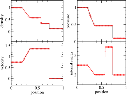
Figure 1: Density, pressure, velocity and internal energy in Test 1 at $t_{0}=0.2$ and $x_{0}=0.3$.

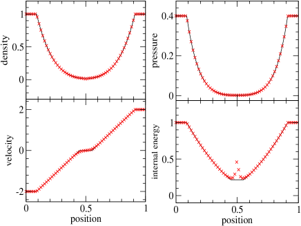
Figure 2: Density, pressure, velocity and internal energy in Test 2 at $t_{0}=0.5$ and $x_{0}=0.5$.

In Fig. 1, we plot the density, pressure, velocity and internal energy of the fluid for Test 1 at $t=0.2$. This test is a modified version of Sod’s test which assesses the entropy satisfaction property of the numerical scheme. The final solution includes a right shock wave, a right-traveling wave and a left sonic rarefaction wave. As seen from the figure, the code can very well preserve the sharp edge of the shock and contact discontinuity. Also, the entropy glitch, which usually appears in low-order schemes in a bump inside the rarefaction, does not appear.

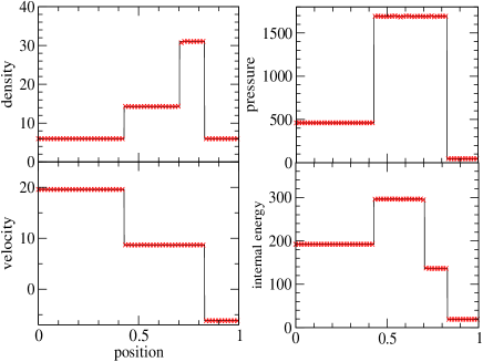
Figure 3: Density, pressure, velocity and internal energy in Test 3 at $t_{0}=0.035$ and $x_{0}=0.4$.

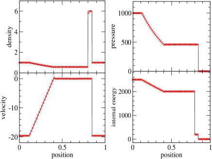
Figure 4: Density, pressure, velocity and internal energy in Test 4 at $t_{0}=0.012$ and $x_{0}=0.8$.

In Fig. 2, we plot similarly the density, pressure, velocity and internal energy of the fluid for Test 2 at $t_{0}=0.15$. This test contains a solution of two rarefaction waves and a stationary contact wave. The solution contains also a low-density region, and it tests how well the code can handle low-density fluid flow. The numerical solution follows the analytic solution very well, except for an undershoot in the velocity near $x=0.5$ and an overestimation by a factor of 2 in the internal energy. Despite these, the performance of the WENO scheme is in general much better than other low-order schemes, which result in spurious oscillations in the velocity field and a larger overestimation in the internal energy (See Toro (2007) for a detailed comparison among different numerical schemes).

In Fig. 3 we plot the test results for Test 3 at $t_{0}=0.035$. This test assesses the robustness of a code in processing strong discontinuities. There are two right-traveling shock waves, a right-traveling contact discontinuity, and a left-traveling shock. It can be seen from the figure that all discontinuities can be resolved without smearing.

In Fig. 4 we plot the density, pressure, velocity and internal energy in Test 4 at $t_{0}=0.012$. This test challenges the code in evolving a slowly-moving or stationary shock discontinuity. The final solution contains a left-traveling rarefaction wave, right-traveling shock wave and a stationary contact discontinuity. The numerical solution largely follows the analytic solution except for a small overshoot in pressure, velocity and internal energy at $x=0.4$ at the edge of rarefaction wave. Also, there are spurious oscillations with a small amplitude in density at $x=0.8$.

Combining these four tests, we can see that our code performs well in treating numerical discontinuity and it can mimic closely the analytic solution. Typical numerical inaccuracies, including the entropy glitches, spurious oscillations and smearing are highly suppressed.

5.2 Two-dimensional Code Test

The one-dimensional tests aim at validating the shock-capturing properties of the WENO scheme under different situations. In this part, we extend the code test to two dimensions. Besides shock-capturing, we also study the numerical diffuseness and the advection of smooth flow of the code. In all tests the polytropic EOS identical to the one-dimensional code tests is used with specific heat ratio $\gamma=1.4$. The Courant number is taken to be 0.5.

Table 4: Fractional changes in mass $\Delta M/M$ and energy $\Delta E/E$ in $Gresho$ test under different resolutions. $L^{1}(p-p_{{\rm ref}})$ is the $L^{1}$ norm of the error in the fluid pressure, with reference to the initial state.

$\Delta$	$N_{x}$	$N_{y}$	$\Delta M/M$	$\Delta E/E$	$L^{1}(p-p_{{\rm ref}})$
$2\times 10^{-2}$	50	50	$2.96\times 10^{-3}$	$4.08\times 10^{-4}$	$4.50\times 10^{-3}$
$1\times 10^{-2}$	100	100	$1.09\times 10^{-3}$	$1.52\times 10^{-4}$	$1.63\times 10^{-3}$
$5\times 10^{-3}$	200	200	$1.49\times 10^{-5}$	$2.10\times 10^{-5}$	$2.89\times 10^{-4}$
$2.5\times 10^{-3}$	400	400	$1.94\times 10^{-6}$	$2.73\times 10^{-6}$	$3.26\times 10^{-5}$

The first test ${Gresho}$ (Gresho, 1990) is to evaluate the code performance in handling time-independent solution, which tests the code in handling advection of smooth functions. The simulation takes place in a square box of $-0.5<x<0.5$ and $-0.5<y<0.5$ with $\Delta$ = 0.02, 0.01, 0.005 and 0.0025 units. The boundary is free everywhere. The simulation time is 3 (code unit). The initial profile is a steady solution given by $\rho=1$ everywhere, $v(r)=5r$, $p(r)=5+25/2r^{2}$ at $0<r<0.2$, $v(r)=2-5r$, $p(r)=9+4{\rm ln}(r/0.2)+25/2r^{2}-20r$ at $0.2<r<0.4$ and $v(r)=0$ and $p(r)=3+4{\rm ln}2$ at $0.4<r<0.5$. Here $r$ is the distance from the origin. Obviously, any departure of the final solution from the initial one must be due to numerical errors from the advection and numerical diffusion. In Fig. 5 we plot the linear density contour plot at $t=3$ for $dt=0.005$. It can be seen that the circular structure is maintained. The outer part remains in uniform pressure. In Table 4 we list the numerical errors in total mass, energy and the $L^{1}$-norm of the fluid pressure. At high resolutions, the results show a third order convergence which is consistent with the order of the time-discretization scheme of the code.

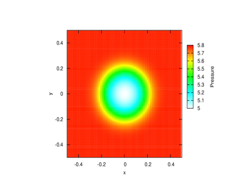
Figure 5: Density contour plot of $Gresho$ test at $t=3$.

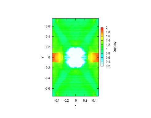
Figure 6: Density contour plot of $Blast$ test at $t=1$.

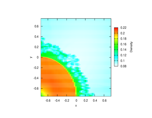
Figure 7: Pressure contour plot of $Explosion$ test at $t=2.667$.

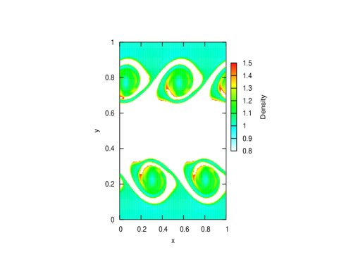
Figure 8: Density contour plot of KH test at $t=1$.

The second test is the Blast test (Toro, 2007) which takes place in a rectangular box of dimensions $-0.5<x<0.5$ and $-0.75<y<0.75$ with reflecting boundaries everywhere. The resolution is $512\times 768$. The initial condition is given by $p=10$ at $r<0.1$ and $p=1$ at $r>0.1$. $\rho=1$ everywhere. This test studies again the capability of the code in handling the low density region, the sharpness of the hydrodynamical instabilities and the shock-shock, or shock-contact discontinuity interactions. In Fig. 6 we plot the linear density contour at $t=1.0$. It can be seen that the symmetry along the x-axis and along the y-axis are preserved. Also, the Richter-Meshkov instability at the boundary of contact-discontinuity in the form of dense filaments or fingers are sharply captured.

The third test is the $Explosion$ test (Toro, 2007) which is very similar to SNIa explosion but without nucleosynthesis. The simulation box is $512\times 512$ with dimensions $0<x<1.5$ and $0<y<1.5$. The inner boundaries are reflecting and the outer boundaries are free. The initial condition is given as an overpressure region at the core, with $p(r)=1.0$ and $\rho(r)=1.0$ at $r<0.4$ and $p(r)=0.1$ and $\rho(r)=0.125$ at $r>0.4$. In Fig. 7 we plot the linear density contours at $t=2.667$. At this moment, the weak reflected shock has arrived inside the shock sphere, and the unstable contact discontinuity of the surface in the form of plumes can be observed. Again, a sharp symmetry with respect to a reflection about $x=y$ can be observed.

The last test is the Kelvin-Helmholtz (KH) test (McNally et al., 2011) which studies the KH instability. The simulation box is $256\times 256$ with dimensions $0<x<1$ and $0<y<1$ with periodic boundaries everywhere. The simulation is done up to $t=2$. The initial condition is that two fluids of different densities flow in opposite directions with a perturbation: $p=1$ everywhere, $\rho=2$ at $0.25<y<0.75$ and $\rho=1$ otherwise. An initial velocity is given as $v_{y}=A(1+{\rm cos}(2\pi x))(1+{\rm cos}(2\pi y))$. In Fig. 8 we plot the linear density contours at $t=1$. The KH instability in the form of spiral shape outside the denser region can be observed.

Combining these four tests, we have seen that the code performs satisfactorily with the desired accuracy and shock-capturing ability in multi-dimensional runs. Also, the code has shown its ability in handling hydrodynamical instabilities, such as the Kelvin-Helmholtz instability.

5.3 Code Test for PTD models

In this part, we return our focus to code test of SNIa explosions using the PTD models. The simulation uses the Helmholtz EOS (Timmes & Swesty, 1999) and all the simulations are done in cylindrical coordinates with 500 grids in each direction. Each grid has a size $\Delta=dr=dz\approx 11$ km. A hydrostatic equilibrium model with a given density is constructed with an isothermal profile of $T=10^{8}$ K and a composition of $X(^{12}$C$)=X(^{16}$O$)=0.5$. The code enforces a minimum density of $10^{5}$ g cm^-3, which is also the atmospheric density. The time step is limited by the Courant-Friedrich-Lewy condition:

$$\Delta t_{{\rm max}}=c_{cfl}\Delta/(c_{s}+|v_{r}|+|v_{z}|),$$ (47)

with $c_{cfl}=0.5$ and $c_{s}$ the local sound speed.

An initial three-finger flame front is imposed, which is comparable with the c3 flame reported in Niemeyer et al. (1996) and Reinecke et al. (1999). The reason we choose this flame front is the same as that in the literature: we want to bypass the slow laminar flame stage and consider the stage where Rayleigh-Taylor instabilities are important. The matter enclosed by the flame front is first burnt. We follow the choice in Niemeyer & Hillebrandt (1995b) to set the initial specific turbulence kinetic energy $q=10^{10}$ cm² s^-2. We also set this value to be the minimum $q$ so as to avoid unphysical result when calculating the production and dissipation of $q$.

Table 5: Simulation setup for the test of PTD models. Lengths are in units of km and densities are in units of $10^{9}$ g cm^-3. Energy is in units of $10^{50}$ erg and masses are in units of solar mass.

Model	$dx$	$\rho_{c}$	mass	radius	$E_{{\rm nuc}}$	$E_{{\rm kin}}$	$M_{{\rm Ni}}$
2D-1a-PTD	11.0	3.0	1.377	1475.0	7.141	2.109	0.320

We tabulate the simulation setups in Table. LABEL:table:TestPTD. We plot in the upper panel of Fig. 9 the total energy against time for Models 2D-1a-PTD. At early time the energy release relies on slow laminar flame, thus the energy growth is slow. At about $t\approx 0.5$ s, the sub-grid turbulence has developed and it boosts the propagation of flame and enhances the consumption of fuel significantly. At about 0.7 s, the nuclear flame has released enough energy to balance the gravitational energy. At $t\approx 0.8$ s, the expansion of the star leads to density decrease at the flame front, which lowers the energy output of the flame as well. So, the total energy levels off and reaches a constant at about $2\times 10^{50}$ erg. Notice that our initial model and related physics are chosen to mimic those of the Model $c3-2d-256$ in Reinecke et al. (2002a). Our results are comparable with theirs, which also give the final energy at $2\times 10^{50}$ erg. In the lower panel, we plot the total turbulence kinetic energy $q$ against time. Similar to the neutrino luminosity, the sub-grid turbulence energy reaches its maximum at around 0.6 s. We plot in the upper panel of Fig. 10 the neutrino luminosity against time. The model shows a single peak at about 0.5 s. This implies that the burning is the most vigorous at that moment. In the lower panel we plot the neutrino energy spectra with energy 1 MeV - 5 MeV as functions of time. In early time, the neutrino energy peaks at 2 MeV. At later time, when the WD starts to expand, the 1 MeV neutrino flux becomes the dominant one.

We also plot in Fig. 11 the time evolution of chemical isotopes. At early time, iron-peaked elements are produced, and a considerable amount of ⁴He is produced. At later time, when the fluid element expands and its temperature drops, ⁴He recombines to ⁵⁶Ni again, and incomplete burning causes the production of a trace amount of IME. The results can also be compared with Model $c3-2d-256$ (Reinecke et al., 2002a) which observes a total of 0.109 $M_{\odot}$ IME and 0.40 $M_{\odot}$ iron-peaked elements. We obtain similar amount of iron-peaked elements but the IME abundance is lower than theirs. This may be due to the difference in approximating the ash composition and the energy release at lower density, which is the main site for the production. We plot in Fig. 12 the flame shape at $t=1$ s. The initial flame is the $c3$ front shape as described in Niemeyer & Hillebrandt (1995b), which is a ”three fingers” shape. The flame shows signatures of hydrodynamical instabilities: the Rayleigh Taylor instability in the form of mushroom shape at the top of the ”fingers” and KH instability in the form of curly shape along the ”fingers”. Injection of fuel into the flame can also be seen between ”fingers”.

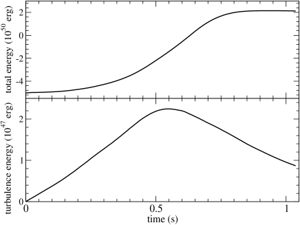
Figure 9: Upper panel: Total energy against time for Model 2D-1a-PTD. Lower panel: Total turbulence kinetic energy against time for the same model.

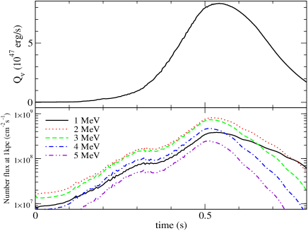
Figure 10: Upper panel: Total neutrino luminosity against time for Model 2D-1D-PTD. Lower panel: Neutrino energy spectra against time for the same model.

5.4 Code test for DDT models

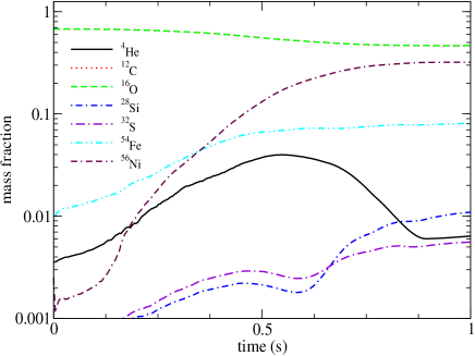
Figure 11: Isotope mass fraction against time for Model 2D-1a-PTD.

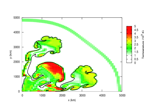
Figure 12: The deflagration and detonation fronts at $t=1$ second for Model 2D-1a-PTD.

In this part we present results for the DDT model. The DDT model is actually a natural continuation of the PTD model for two reasons. First, before the detonation starts, the evolution is exactly the same as the PTD model. Second, the criterion for the first detonation spot relies on the local turbulence that the flame width $\delta$ equals the Gibson length, also known as the turbulence length scale $l_{{\rm Gib}}$, below which the laminar flame is the dominant propagation channel. Mathematically, we have

$$\delta=l_{{\rm Gib}}=\Delta(v_{{\rm lam}}/2q)^{3/2}.$$ (48)

The flame width is obtained from the results by solving the deflagration wave, as described in Appendix A, which is a function of density. We note that this relation, which is equivalent to the Karlovitz number $Ka=1$, only states that turbulence starts to destroy the flame front. But as argued in Niemeyer & Woosley (1997), this mechanism can allow the heat from the ash to be transported to the fuel much more efficiently than only by conduction. This creates a much wider region with sufficient temperature for carrying out carbon burning simultaneously, which is believed to be one of the keys for triggering the detonation. In the simulation, whenever there is a grid on the flame front satisfying this criterion, a spherical detonation spot of radius $\Delta$ is artificially placed and evolved similarly as the deflagration front. However, because the deflagration front has burnt partially the stellar material in the core, whenever the detonation front reaches the flame surface, we assume that the detonation front stops.

Table 6: Simulation setup for the test of DDT models. Lengths are in units of km and densities are in units of $10^{9}$ g cm^-3. Energy is in units of $10^{50}$ erg and masses are in units of solar mass. $t_{{\rm tran}}$ is the first DDT time in seconds.

Model	$dx$	$\rho_{c}$	mass	radius	$E_{{\rm nuc}}$	$E_{{\rm kin}}$	$M_{{\rm Ni}}$	$t_{{\rm tran}}$
2D-1a-DDT	11.0	3.0	1.377	1475.0	15.651	10.618	0.733	0.70

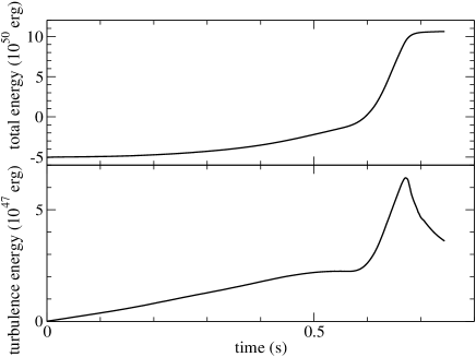
Figure 13: Upper panel: Total energy against time for Model 2D-1a-DDT. Lower panel: Total turbulence kinetic energy against time for the same model.

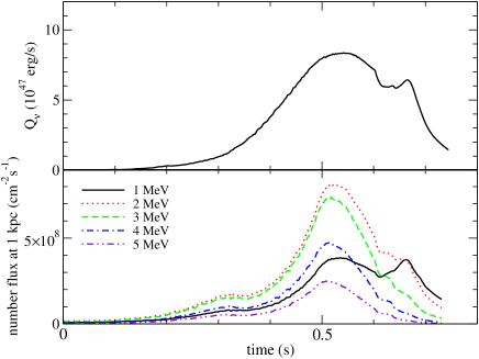
Figure 14: Upper panel: Total neutrino luminosity against time for Model 2D-1a-DDT. Lower panel: Neutrino energy spectra against time for the same model.

We carry out tests for models using DDT and we tabulate the input parameters and final explosion energetics in Table LABEL:table:TestDDT. The explosion energetics can be compared with Model $Z3a$ in Golombek & Niemeyer (2005). But the major difference between Model $Z3a$ and ours is that the former one allows the detonation front to pass through burnt regions, which is not allowed in ours in view of some direct numerical simulations of the instability of the shock front in the presence of ash product (Maier & Niemeyer, 2006). They reported $E_{{\rm nuc}}=14.4\times 10^{50}$ erg with $E_{{\rm kin}}=8.70\times 10^{50}$ erg. The DDT transition time is 0.85 s and the final amount of ⁵⁶Ni in their model is 0.65 $M_{\odot}$. Our model shows a higher energy release, a higher ⁵⁶Ni production and an earlier trigger in DDT.

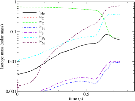
Figure 15: Isotope mass fraction against time for model 2D-1a-DDT.

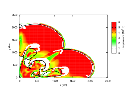
Figure 16: The deflagration and detonation fronts of Model 2D-1a-DDT at $t=1.00$. The temperature distribution is represented in different colours.

In the upper panel of Fig. 13, we plot the total energy against time for Model 2D-1a-DDT. Prior to the detonation front being triggered, the evolution is identical to that of the PTD model. By comparing with Model 2D-1a-PTD, we see that our model is consistent with models in the literature that most energy is released by the detonation front instead of the deflagration front, which is also needed to match the ejecta velocity with the observed SNIa. In the lower panel, we plot the total turbulence kinetic energy. The turbulence constantly develops as the fluid motion becomes chaotic, and then it drops slightly when the WD expands. Turbulence grows again when the detonation is launched, which reaches its maximum as the explosion has burnt all the fuel in the WD. But it then drops sharply due to the rapid expansion of the star.

In the upper panel of Fig. 14 we plot the neutrino luminosity of Model 2D-1a-DDT. The neutrino luminosity is decreasing when the detonation is just started. But it goes up again due to a large amount of matter being thermalized. In the lower panel we plot the neutrino energy spectra with energy 1 MeV - 5 MeV as functions of time. Again the number flux of each energy band shows a rise after DDT has started and after $t=0.7$ s, the 1 MeV neutrino number flux exceeds the other four fluxes of higher energy bands. We also plot the isotope abundances against time in Fig. 15. The early time evolution is comparable to the PTD model. After the detonation has started, much more iron-peaked elements and IME are produced, leaving trace amounts of ¹²C and ¹⁶O. At last, we plot deflagration and detonation flame front at $t=1$ s in Fig. 16. The flame front is shaped by the fluid flow, that ”mushroom caps” and injection of fuel can be observed from the flame front. The detonation front first starts at the outermost part of the flame front, which develops at first spherically, but then loses its symmetry when the front encounters another detonation front and the deflagration front.

6 Observational Prediction

We have demonstrated in previous sections that our hydrodynamics code can provide explosion energetics comparable with models in the literature. To further study the hydrodynamics result, we perform a series of post-processing procedures to extract SNIa observables, including the nucleosythesis yields by the tracer particle method and the bolometric light curve using a moment-integrated radiative transfer code.

6.1 Nucleosynthesis Products

We use the tracer particle method to keep track of the density and temperature of each fluid parcel, which represents a fixed amount of mass elements in the fluid. We repeat the 2D-1a-DDT model but with different numbers of tracer particles. We study its numerical convergence by adjusting the initial radial and angular separation of the fluid parcels. In the first test, we use a simple 19-isotope network with a fixed output time of hydrodynamics properties at 0.025 s. We tabulate the nucleosynthesis yields in Table LABEL:table:Run2D_tracer_results. We also include the chemical composition from the hydrodynamics run for comparison. In general, the post-processed yields are different from that of the hydrodynamics run in two ways; the final distributions of ¹²C and ¹⁶O are not the same in the post-processed results. This is related to the slow-burning in the low density regime, which is not assumed in the deflagration wave product. This also affects the IME distribution so that much higher mass fractions of ²⁸Si and ³²S are observed. Second, the amount of iron-peaked elements are drastically different in that the ⁵⁴Fe are generally lower, showing that lower amount of matter has reached nuclear statistical equilibrium for a complete burning comparing to the expectation from the deflagration wave solution. We also compare how the number of tracers along each direction affects the final results. We find that for $N=80^{2}$ the changes in the final yields differ by less than 1 $\%$, while more abundant isotopes such as ⁵⁴Fe and ⁵⁶Ni generally converge faster than less abundant elements such as ⁴⁰Ca and ⁴⁴Ti.

Table 7: Masses of all isotopes at the end of simulations for different numbers of tracer particles $N=40^{2}$, $80^{2}$ and $160^{2}$. The approximate yields from the hydrodyanmics run are also included for comparison. The 19-isotope network is used. The record time is fixed at $t=0.025$ s. All quantities are in units of solar mass.

Isotope	Hydro	$N=40^{2}$	$N=80^{2}$	$N=160^{2}$
12C	$6.68\times 10^{-2}$	$1.61\times 10^{-2}$	$1.61\times 10^{-2}$	$1.60\times 10^{-2}$
16O	$6.68\times 10^{-2}$	$3.74\times 10^{-2}$	$4.36\times 10^{-2}$	$4.33\times 10^{-2}$
24Mg	$1.60\times 10^{-5}$	$8.36\times 10^{-3}$	$1.11\times 10^{-2}$	$1.06\times 10^{-2}$
28Si	$9.17\times 10^{-3}$	$1.97\times 10^{-1}$	$1.99\times 10^{-1}$	$1.98\times 10^{-1}$
32S	$9.93\times 10^{-3}$	$9.22\times 10^{-2}$	$9.16\times 10^{-2}$	$9.08\times 10^{-2}$
36Ar	$6.90\times 10^{-3}$	$1.93\times 10^{-2}$	$1.90\times 10^{-2}$	$1.88\times 10^{-2}$
40Ca	$1.27\times 10^{-2}$	$1.82\times 10^{-2}$	$1.78\times 10^{-2}$	$1.76\times 10^{-2}$
44Ti	$3.80\times 10^{-4}$	$9.96\times 10^{-5}$	$9.73\times 10^{-5}$	$9.66\times 10^{-5}$
48Cr	$2.91\times 10^{-2}$	$8.71\times 10^{-4}$	$8.46\times 10^{-4}$	$8.39\times 10^{-4}$
52Fe	$4.20\times 10^{-2}$	$2.10\times 10^{-2}$	$2.07\times 10^{-2}$	$2.06\times 10^{-2}$
54Fe	0.368	0.100	$9.89\times 10^{-2}$	$9.99\times 10^{-2}$
56Ni	0.733	0.836	0.831	0.831

6.2 Bolometric Light Curve

Using the hydrodynamics results from models as we have obtained in Sections 5.3 and 5.4, we can predict the expected observational signals of these explosions. We plot in Fig. 17 the bolometric light curves for Models 2D-1a-DDT using the one-dimensional radiative transfer code. The nickel abundance and its distribution have stronger effects on the peak luminosity and width. We obtain a peak luminosity log₁₀ $L_{{\rm peak}}=43.1$ with a drop of the absolute magnitude at 15 days after maximum $\Delta m_{15}=0.58$. A mild but observable secondary bump can be seen at about Day 30, showing that the photosphere has receded inside the iron layer. Beyond Day 40, when ⁵⁶Co decay becomes the dominant energy source, the curve drops at a constant rate.

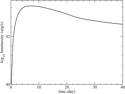
Figure 17: Bolometric light curves of Model 2D-1a-DDT.

7 Discussion and Conclusion

In this paper, we have presented a two-dimensional Eulerian hydrodynamics code for modeling SNIa using cylindrical coordinates with the level-set method as the flame capturing scheme. We also included the sub-grid turbulence for modeling turbulent flame and a neutrino subroutine for computing the corresponding neutrino spectra. We also used a tracer particle scheme for nucleosynthesis and developed a moment-integrated radiative transfer code for computing the bolometric light curve. We have preformed benchmark tests in one and two dimensions to evaluate the accuracy and robustness of the code. Also, we have studied the SNIa explosion using the PTD and DDT models. The nucleosynthesis details and the bolometric light curves of our simulation models are comparable to those similar explosion models presented in the literature.

However, it should be noted that a consistent comparison with models in other works are difficult for two reasons. First, there are different numerical treatments for the same physical process. For example, in earlier works the effective flame propagation speed is chosen to be the maximum of various flame propagation mechanisms, while in later works the transition of the flame from laminar to turbulent is based on analytic models (Pocheau, 1994). However, how the flame propagation varies with local turbulence is not yet exactly known. Second, each code has its own prescription for the input physics, such as the EOS and the nuclear reaction network, while some processes, such as the nucleosynthesis and the turbulence model, depend on these models. For example, we use the same EOS presented in Timmes & Swesty (1999) as the FLASH code (Calder et al., 2002), but their model does not include the effects of sub-grid turbulence. Also, our nuclear energy production depends on the choice of EOS. We directly use a nuclear reaction network to calculate the energy released by the deflagration and detonation waves, while in Schmidt et al. (2005) all materials are assumed to be burnt into nuclear statistical equilibrium at high densities and only up to ²⁴Mg at low densities. The difference has a subtle effect on the explosion since the produced energy may boost the fluid motion for the creation of sub-grid velocity fluctuations and at the same time makes the star expand. The produced energy then affects the local density which consequently affects the energy release again. Therefore it is difficult to carry out a quantitative comparison when the hydrodynamics, flame physics and nucleosynthesis are coupled.

In future work, we plan to include other numerical components, such as the advection-diffusion-reaction scheme and other models of sub-grid turbulence. By comparing the results of these numerical components we may better understand their roles in the explosion, as well as the limitation and validity regimes of these models. Also, as a natural continuation of our previous work (Leung et al., 2013), the effects of dark matter will be included into the dynamics. We plan to examine whether the presence of dark matter affects the role of SNIa as a standard candle, which is critical in the discovery of dark energy and measurements of cosmological distances.

8 Acknowledgment

We thank K.-W. Wong for his development of a 1D WENO solver based on which our 2D SNIa code is constructed. We also thank F. X. Timmes for his open-source codes of the Helmholtz EOS, nuclear reaction network and neutrino emission. This work is partially supported by a grant from the Research Grant Council of the Hong Kong Special Administrative Region, China (Project No. 400910). SCL is supported by the Hong Kong Government through the Hong Kong PhD Fellowship.

Appendix A Deflagration wave

In Sections 2.2 and 3.2 we mentioned that deflagration and detonation are coupled to the hydrodynamics as energy sources. Here we describe the governing equations for deflagration, how they are solved to obtain the results.

Deflagration is one of the combustion processes where electron scattering is the major heat transport mechanism. The process is so slow that the fluid remains almost isobaric. The wave structure and the flame speed are studied in Timmes & Woosley (1992). At least four methods can be used to study the structure of deflagration wave. They include direct simulations, diffusion approximations, eigenvalue method and variational approximations, arranged in descending order of information provided. Direct simulation is the computationally most expensive method, but is the most accurate one, because no assumption is made in the evolution equations. On the other hand, variational approximation is the least accurate as it gives only a lower bound of the flame speed and reveals no information about the flame structure. In our simulations, we use the diffusion approximations in finding the flame structure and its corresponding speed, which is shown to be a good approximation due to the slow propagation of flame compared with the much faster sound speed.

The diffusion approximation starts from the general Euler equations in spherical coordinate and Lagrangian formulation, namely,

$$\frac{\partial m}{\partial r} = 4\pi r^{2}\rho,$$ (49)

$$\frac{Dv}{Dt} = -4\pi r^{2}\frac{\partial P}{\partial m}-\frac{GM}{r^{2}},$$ (50)

$$\frac{D\epsilon}{Dt}+P\frac{\partial(1/\rho)}{\partial t} = \frac{1}{\rho}\frac{\partial}{\partial r}\left(\chi\frac{\partial T}{\partial r}\right)+\dot{q},$$ (51)

$$\dot{q} = N_{{\rm A}}\sum_{i}\frac{DY_{i}}{Dt}B_{i},$$ (52)

$$\frac{DY_{i}}{Dt} = \sum_{j,k}-Y_{i}Y_{j}\lambda_{jk}(i)+Y_{l}Y_{k}\lambda_{kj}(l).$$ (53)

$B_{i}$ and $Y_{i}$ are the binding energy and the number fraction of isotope $i$. $\lambda_{jk}$ is the reaction rate of nuclear reaction from isotope $j$ to $k$. Other variables have the the same physical meaning as in the main text. The derivative $D/Dt$ is the time derivative in the frame moving with the fluid. The diffusion approximation then assumes that the fluid has always the same pressure. Gravity is neglected because the typical size of deflagration reaction zone is much smaller than the density scale height. This means that the velocity equation Eq. (50) can be neglected.

In the heat diffusion term on the right hand side of Eq. (51) $\chi$ is the total thermal conductivity, which consists of contributions from both electron and photon conductivities

$$\chi=\chi_{e}+\chi_{\gamma}.$$ (54)

Photon conductivity can be exactly found as $\chi_{\gamma}=4acT^{3}/3\kappa\rho$, with $a=7.5657\times 10^{-15}$ erg cm^-1 K^-4 being the radiation constant, $c$ being the speed of light and $\kappa$ being the opacity.

To find the electron conductivity, we follow the prescription of Khokhlov et al. (1997). First we have $\chi_{e}$ expressed in terms of the effective electron collisional frequency $\nu_{e}$

$$\chi_{e}=4.09\times 10^{9}T\frac{x^{3}}{\sqrt{1+x^{2}}}\left(\frac{10^{16}}{\nu_{e}}\right){\rm ergs~{}cm^{-1}s^{-1}K^{-1}},$$ (55)

with $x=p_{F}/m_{e}c$ being the dimensionless Fermi momentum. The electron collisional frequency can be separated into ion-electron and electron-electron collisional frequencies by

$$\nu_{e}=\nu_{ee}+\nu_{ei}.$$ (56)

The electron-ion collisional frequency is given by

$$\nu_{ei}=1.78\times 10^{16}\sqrt{1+x^{2}}\frac{\bar{Z}\Lambda}{\bar{A}Y_{e}},$$ (57)

with $\bar{A}$ being the mean atomic mass and $\bar{Z}$ being the mean atomic number. $Y_{e}$ is the electron fraction and $\Lambda$ is the Coulomb logarithm.

$$\Lambda = \ln\left[\left(\frac{2\pi Z}{3}\right)^{1/3}\sqrt{\frac{3\Gamma+3}{2}}\right]-\frac{x^{2}}{2(1+x^{2})}+$$ (58)

$$\frac{\pi}{2}\alpha\beta^{2}\frac{1+1.3\alpha}{1+\alpha^{2}(0.71-0.54\beta^{2})}.$$

Here, $\Gamma=2.275\times 10^{5}\bar{Z}^{5/3}(\rho Y_{e})^{1/3}/T$, $\beta=x/\sqrt{1+x^{2}}$ and $\alpha=Z/137\beta$.

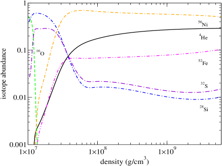
Figure 18: Isotope abundances against density for 13 isotopes. See the text for the lists of elements.

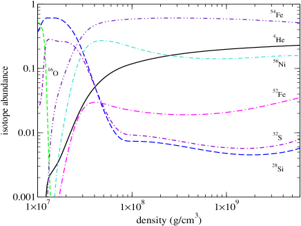
Figure 19: Isotope abundances against density for 19 isotopes. See the text for the lists of elements.

Similarly, we have the electron-electron collision frequency as a function of temperature and density

$$\nu_{ee}=0.511T^{2}\frac{x^{3/2}}{(1+x^{2})^{5/4}}J(y)~{}{\rm s^{-1}},$$ (59)

with $y=\sqrt{3}T_{pe}/T$. $T_{pe}$ is the electron-plasma temperature given by

$$T_{pe}=3.307\times 10^{8}\frac{x^{3/2}}{(1+x^{2})^{1/4}}~{}{\rm K}.$$ (60)

$J(y)$ is an integral that cannot be evaluated analytically and is given numerically by

$$J(y)=\frac{1}{3}\left(\frac{y}{1+ay}\right)^{3}\ln\left(\frac{2+by}{y}\right),$$ (61)

where $a=0.113$ and $b=1.247$.

Using these information, we find numerically the deflagration wave propagation speed, the energy production and the ash composition. To start the deflagration wave, we follow the prescription in Timmes & Woosley (1992). We first ignite the innermost grid cells, setting its initial temperature sufficient for nuclear runaway. Then we start the evolution and gradually a steady deflagration wave forms. The laminar flame velocity can be obtained by studying the motion of the steady wave structure. The ash composition is obtained from the regions swept by the deflagration wave. The internal energy production is calculated by comparing the initial and final specific internal energy.

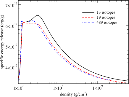
Figure 20: Specific internal energy production against density for 13, 19 and 489 isotopes. See the text for the lists of elements.

As shown in Timmes & Woosley (1992), the laminar flame velocity can be well approximated by

$$v_{{\rm lam}}=92.0~{}{\rm km~{}s}^{-1}\left(\frac{\rho}{10^{9}~{}{\rm g~{}cm}^{-3}}\right)^{0.805}\left(\frac{X_{C}}{0.5}\right)^{0.5},$$ (62)

with $X_{C}$ being the mass fraction of ¹²C.

We plot in Figs. 18 and 19 the ash composition against fuel density using 13-isotope and 19-isotope networks. At low density $\rho\sim 10^{7}$ g cm^-3, only carbon is consumed. Oxygen remains barely unchanged. Magnesium and silicon are the major products. At $\rho\sim 5\times 10^{7}$ g cm^-3, oxygen is also consumed, with silicon and sulphur being the major products. At density around $10^{8}$ g cm^-3, iron and nickel become prominent. Also helium is produced due to photo-disintegration. ⁵⁴Fe is the major product when it is included in the nuclear reaction network, which is absent in the 13-isotope network.

In Fig. 20 we plot the energy release against fuel density using 13-, 19- and 489-isotope networks. The specific internal energy production (SIEP) is in the order of $10^{17}$ erg. At low density $\rho\sim 10^{7}$ g cm^-3, SIEP increases with density and the oxygen mass fraction decreases. This is because the reaction rate increases with density. At density above $5\times 10^{7}$ g cm^-3, SIEP drops. This does not mean less fuel is consumed. As mentioned in Reinecke et al. (2002a), at high temperature, the highly endothermic photo-disintegration ⁵⁶Ni $\rightarrow 14^{4}$He becomes important, which compensates for the rise of SIEP.

Appendix B Detonation Wave

To determine the wave structure, we follow the prescription in Sharpe (1999). We first find the thermodynamics state of shocked fluid from a given state. Then, using the shocked state as an initial condition, the wave structure can be obtained by solving the steady state limit of Euler equations with nuclear reactions.

For the first part, the upstream and downstream states are related by the Rankine-Hugoniot conditions

$$\rho u=\rho_{0}D,$$ (63)

$$p+\rho v^{2}=p_{0}+\rho_{0}D^{2},$$ (64)

$$\epsilon+\frac{p}{\rho}+\frac{v^{2}}{2}=\epsilon_{0}+\frac{p_{0}}{\rho_{0}}+\frac{D^{2}}{2}.$$ (65)

Quantities with a subscript 0 are the upstream (unshocked) state. $D$ is the outflow velocity. Both $\epsilon_{0}(\rho_{0},T_{0},X_{0})$ and $p(\rho_{0},T_{0},X_{0})$ are dependent on given density, temperature and composition. In particular, $\rho_{0}$ and $T_{0}$ are free parameters, but the actual results are insensitive to $T_{0}$, because the upstream electrons are highly degenerate. $X_{0}$ is the composition of fuel, namely 0.5 $X_{C}$ and 0.5 $X_{O}$. In general, the final composition $X$ is a set of quantities (depending on the choice of isotopes) to be determined.

After having the post-shock state, we determine the reaction zone size and the ash composition by assuming a one-dimensional planar and steady flow, namely

$$v\frac{d\rho}{dx}+\rho\frac{du}{dx}=0,$$ (66)

$$\rho v\frac{du}{dx}+\frac{dp}{dx}=0,$$ (67)

$$\frac{d\epsilon}{dx}-\frac{p}{\rho^{2}}\frac{d\rho}{dx}=0,$$ (68)

$$\frac{dX}{dx}=\frac{R}{v},$$ (69)

where $R$ is the reaction rate. Then, using

$$dp=\left(\frac{\partial p}{\partial\rho}\right)_{T,X}d\rho+\left(\frac{\partial p}{\partial T}\right)_{\rho,X}dT+\sum^{N}_{i=1}\left(\frac{\partial p}{\partial X_{i}}\right)_{\rho,T}dX_{i},$$ (70)

and

$$d\epsilon=\left(\frac{\partial\epsilon}{\partial\rho}\right)_{T,X}d\rho+\left(\frac{\partial\epsilon}{\partial T}\right)_{\rho,X}dT+\sum^{N}_{i=1}\left(\frac{\partial\epsilon}{\partial X_{i}}\right)_{\rho,T}dX_{i},$$ (71)

the Euler equations with nuclear reactions in the steady state limit can be reduced to

$$\frac{d\rho}{dx} = -\frac{\rho a^{2}_{f}}{v}\frac{{\bf\sigma}\cdot{\bf R}}{\eta},$$ (72)

$$\frac{dT}{dx} = \left(\frac{\partial p}{\partial T}\right)^{-1}_{\rho,X}\left\{\left[u^{2}-\left(\frac{\partial p}{\partial\rho}\right)_{T,X}\right]\frac{d\rho}{dx}-\right.$$ (73)

$$\hskip 28.45274pt\left.\sum^{N}_{i=1}\left(\frac{\partial p}{\partial X_{i}}\right)_{\rho,T,X_{j\neq i}}\frac{dX_{i}}{dx}\right\},$$

$$\frac{dY}{dx} = \frac{R}{v},$$ (74)

where

$$\eta=a^{2}_{f}-v^{2}$$ (75)

is the sonic parameter,

$$a^{2}_{f}=\left(\frac{\partial p}{\partial\rho}\right)_{T,X}+\left[\frac{p}{\rho^{2}}-\left(\frac{\partial\epsilon}{\partial\rho}\right)_{T,X}\right]\left(\frac{\partial p}{\partial T}\right)_{\rho,X}\left(\frac{\partial\epsilon}{\partial T}\right)^{-1}_{\rho,X}$$ (76)

is the sound speed of constant composition (also known as frozen sound speed) and

$$\sigma_{i} = \frac{1}{\rho a^{2}_{f}}\left\{\left(\frac{\partial p}{\partial X_{i}}\right)_{\rho,T,X_{j\neq i}}-\left(\frac{\partial p}{\partial T}\right)_{\rho,X}\left(\frac{\partial\epsilon}{\partial T}\right)^{-1}_{\rho,X}\times\right.$$ (77)

$$\left.\left[\left(\frac{\partial\epsilon}{\partial X_{i}}\right)_{\rho,T,X_{j\neq,i}}-\left(\frac{\partial q}{\partial X_{i}}\right)_{X_{j\neq i}}\right]\right\}$$

is the thermicity constant, such that ${\bf\sigma}\cdot{\bf R}$ is the thermicity.

Eq. (74) can be integrated into the reaction zone. Notice that there are actually two types of detonation structure implied from these equations. One type is that throughout the detonation wave both $\eta$ and thermicity are positive, while the other type is that both quantities are both positive or negative simultaneously. The first type is the well-known Chapman-Jouguet (CJ) detonation, while the second type is called the supported pathological (SP) detonation.

CJ detonation occurs at low density ($\rho<2\times 10^{7}$ g cm^-3). The boundary condition is given by $\eta={\bf\sigma}\cdot R=0$ at $x\rightarrow\infty$. This corresponds to the ash propagating at frozen sound speed at the point where no more nuclear reaction can proceed.

For SP detonation ($\rho>2\times 10^{7}$ g cm^-3), the integration is divided into two sections. First, we integrate the equation close to $\eta\rightarrow 0$ (while thermicity needs not to be zero at that position). Assume $\eta=0$ at $x=x_{p}$ and we have integrated up to $x=x_{p}-\Delta x_{p}$, by making use of the symmetry of Eqs. (74) from the zero-velocity point and the continuity of thermodynamics variables, we obtain the post-zero-point states at $x=x_{p}+\Delta x_{p}$, where

$$\rho(x_{p}+\Delta x_{p})=\rho(x_{p}-\Delta x_{p}),$$ (78)

and

$$T(x_{p}+\Delta x_{p}) = T(x_{p}-\Delta x_{p})-$$ (79)

$$\sum^{N}_{i=1}\left(\frac{\partial p}{\partial X_{i}}\right)_{\rho,T,X_{j\neq i}}\frac{dX_{i}}{dx}(2\Delta x_{p}).$$

After the above transition, the integration can be carried on again until no net nuclear reaction continues. To determine the correct eigenvalue, we require $\eta={\bf\sigma}\cdot R=0$ at the same position.

Appendix C Flame Capturing using the Point-Set method

In two-dimensional simulations, the flame front is represented by a system of line segments. The point-set method (see for example in (Glimm et al., 1981; Glimm & McBryan, 1985; Glimm et al., 1987; Glimm et al., 1988; Glimm et al., 2002) for applications in two-dimensional systems, (Glimm et al., 1999, 2000, 2003) for applications in three-dimensional systems and (Zhang, 2009) for its application in SNIa modeling.) introduces a set of pseudo-particles, which form a line by assuming that the nearest neighbors are linked. Similar to the level-set method, the particles are transported by the fluid advection with a speed $\vec{v}_{{\rm fluid}}$ and its own propagation with velocity $v_{{\rm flame}}\hat{n}$ , such that

$$\vec{v}_{{\rm node}~{}i}=v_{{\rm flame}}\hat{n}_{i}+\vec{v}_{{\rm fluid}}.$$ (80)

$\hat{n}_{i}$ is the unit normal vector of the flame front pointing from the $i$-th node towards the fuel. The fluid velocity is given directly by the Euler equations. The flame propagation depends on the fluid density and the local normal direction of flame front pointing towards the fuel. The normal of a node is defined by the positions of its closest neighboring nodes. For example, given a node $i$ with position $(x_{i},y_{i})$, with a distance to its next node $i+1$ given by

$$d_{i,i+1}=\sqrt{(x_{i}-x_{i+1})^{2}+(y_{i}-y_{i+1})^{2}},$$ (81)

we define the normal direction of the line segment formed by the nodes $i$ and $i+1$ by

$$\hat{n}_{i}=\left(-\frac{y_{i+1}-y_{i}}{d_{i,i+1}},\frac{x_{i+1}-x_{i}}{d_{i,i+1}}\right).$$ (82)

Notice that whether the normal vector pointing towards the fuel or ash is arbitrary. In our study, we choose the former one.

After all node velocities are found, the positions are updated by

$$\vec{x}_{{\rm node~{}(new)}}=\vec{x}_{{\rm node~{}(old)}}+\vec{v}_{{\rm node}}\Delta t_{{\rm node}}.$$ (83)

There is no accelerating term for the node because the particles serve only as markers of the deflagration front for computing the change in energy and isotopes, which do not interact with the fluid directly.

The time step may not be the same as that of the hydrodynamics one, because the resolution of the point-set method and the hydrodynamics are independent. In general, we require

$$\Delta t_{{\rm node}}=C\frac{l_{{\rm min}}}{v_{{\rm node}}},$$ (84)

with $C$ a positive number smaller than unity and $l_{{\rm min}}$ the minimum distance between neighboring nodes.

Apart from $l_{{\rm min}}$, there are two more parameters controlling the point-set resolution, $l_{{\rm max}}$ and $l_{{\rm merge}}$. They define the inter-node maximum separation and merging distance between non-neighboring nodes. These parameters are essential in maintaining a consistent resolution of the surface during the evolution, because the distance between linked nodes can become too far or close, or there can be lines crossing each other. These phenomena occur frequently when the fluid motion is turbulent. In those cases, node addition, removal or reconnection is needed. Notice that in the literature, node reconnection is also known as surface splitting/merging in the context of multi-dimensional simulations.

To check whether there are regions which are overcrowded or underpopulated with nodes, we calculate the distance between nearest neighbors. Given two nodes $i$ and $i+1$ with separation $d_{i,i+1}$, if $d_{i,i+1}<l_{{\rm min}}$, one of the node is moved to a new position $((x_{i}+x_{i+1})/2,(y_{i}+y_{i+1})/2)$, while the other node is deleted; on the other hand, if $d_{i,i+1}>l_{{\rm max}}$ an extra node between node $i$ and $i+1$ is inserted at position $((x_{i}+x_{i+1})/2,(y_{i}+y_{i+1})/2)$. See Fig. 21 for a graphical illustration of the above operations.

To avoid lines from crossing each other, we locate all node pairs which are not connected but are potentially close enough to form a line. We first identify the nodes which lie on the same or neighboring grids, based on the same Eulerian grid of the hydrodynamics, then the separations of this group of nodes are computed. When any pair of non-neighboring nodes satisfies $d_{i,j}<l_{{\rm merge}}$ for some $i$ and $j$ that $|i-j|\neq 1$, we reconnect the nodes as shown in Fig. 21 and change the topology of the surface. In principle, the aim is that the new surface may preserve the node position but the new surfaces will propagate away from each other, so that no entanglement can be formed in the coming time steps. In practice, for a line without entanglement, there exists only one unpaired node $j$ with any node $i$ such that $d_{i,j}\leq l_{{\rm max}}$. However, when surfaces are going to split or merge, there is more than one of such candidate, which means that there is more than one way to form a line. To decide which node should be chosen, we use the above principle to connect the node such that a concave surface is obtained. Geometrically, the normal vectors on the new surfaces are converging. See Fig. 22 for a graphical description. We remark that how the surfaces merge is unique in two-dimensional simulations because all nodes have at most two neighbors for forming line segments. This property is not true for three-dimensional models because the surface is usually represented by triangular patches, which means that each node always has multiple connections with neighboring nodes. Thus, the geometry of the surface, such as the curvature, will depend on how nodes are connected.

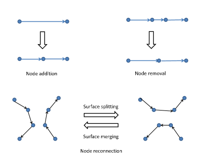
Figure 21: Illustration on node addition, removal and reconnection. The arrows between nodes stand for the pointer from one node variable to the next node variable.

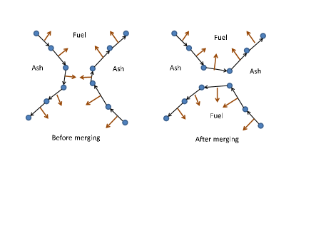
Figure 22: Illustration on how node merging can pervent two lines from crossing each other. The arrows on the line stand for the normal direction of the flame surface.

The three parameters, $l_{{\rm max}}$, $l_{{\rm min}}$ and $l_{{\rm merge}}$ are interrelated. First, we require $l_{{\rm max}}=2l_{{\rm min}}$. This is because we do not want any repetitive loop of node addition or removal to take place, that means, after adding (removing) a new node between any two nearest-neighbors, the new configuration does not have nodes which are too close to (far from) each other according to the criteria. Similarly, we require $l_{{\rm merge}}\leq l_{{\rm max}}$ to avoid entangled lines in simulations. Since the point-set method has a time step that prevents a node from moving further than $l_{{\rm max}}$, we thus choose $l_{{\rm merge}}=l_{{\rm max}}$.

We compare the performance of the level-set algorithm with the point-set algorithm. The level-set algorithm is known to be unable to track the flame consistently when the flame propagates much slower than the fluid flow. The flame surface is dominated by the turbulent flow where the flame is supposed to show a convoluted and elongated structure shaped by the fluid. But the level-set method can only preserve structure with a size greater than the grid size. Therefore, the small-scale structure cannot be tracked and a detached flame in forms of bubbles is obtained. To maintain the consistency of the level-set algorithm in SNIa simulations, flame acceleration schemes are needed (Calder et al., 2007). To address this problem, we compare the flame structure in the laminar flame limit by using the two algorithms. We present the simulation models in Table LABEL:table:TestLine. The hydrodyanmics is the same as those in PTD tests and DDT tests. The hydrodynamics is done with a configuration similar to Section 5.3 with an array of $500\times 500$ in cylindrical coordinates with uniform grid size $\Delta=11$ km.

Table 8: Simulation setup for the test of flame capturing scheme. Lengths are in unit of code unit and densities are in unit of $10^{9}$ g cm^-3.

Model	scheme	$l_{{\rm max}}$	$l_{{\rm min}}$	$l_{{\rm merge}}$	$\rho_{c}$
LSM-1	level-set	3.0	1.5	3.0	3
PSM-1-2	point-set	2.0	1.0	2.0	3
PSM-1-3	point-set	3.0	1.5	3.0	3
PSM-1-4	point-set	4.0	2.0	4.0	3

In Fig. 23 we plot the total energy against time for Models LSM-1, PSM-1-2, PSM-1-3 and PSM-1-4. As expected, the laminar deflagration cannot successfully unbind the star. All four models perform similarly in early time. The model PSM-1-3 is the most similar one to LSM-1. At later time, the level-set method predicts less energy as compared to other three models.

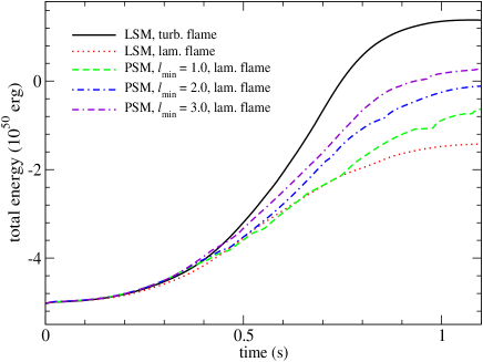
Figure 23: Total energy against time for Models LSM-1, PSM-1-2, PSM-1-3, PSM-1-4. See Table LABEL:table:TestLine for the configurations.

In Figs. 24, 25 26 and 27 we plot the flame front of Models PSM-1-2, PSM-1-3, PSM-1-4 and LSM-1, respectively at $t=1.0$ s. By comparing Models PSM-1-2, PSM-1-3 and PSM-1-4, it shows that the resolution of point-set method affects the performance in two ways: First, it contributes to the fine details of RT and KH instabilities, which enlarge the local flame area; second, the algorithm allows an extremely elongated flame structure and an injection of fuel into burnt region in the sub-grid scale. This property is important for keeping information of the flame surface as much as possible, which maintains the fuel burning rate.

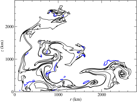
Figure 24: Flame front of Model PSM-1-2 at $t=1.00$ s.

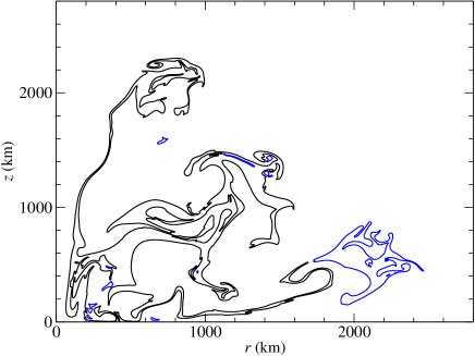
Figure 25: Flame front of Model PSM-1-3 at $t=1.00$ s.

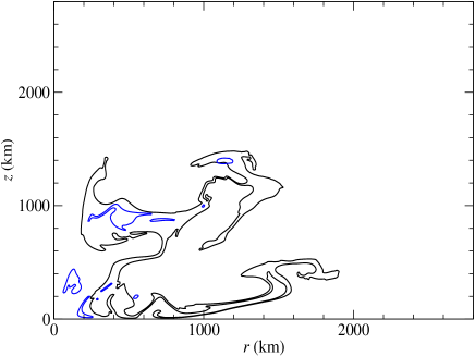
Figure 26: Flame front of Model PSM-1-4 at $t=1.00$ s.

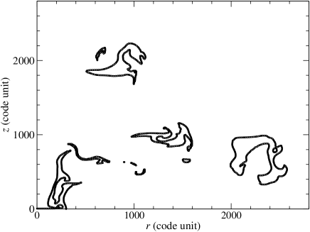
Figure 27: Flame front of Model LSM-1 at $t=1.00$ s.

We compare the point-set method and the level-set method by comparing the flame surface of LSM-1 and PSM-1-4. Both methods give thin flame shape. The point-set method shows a largely connected structure with some fuel regions surrounded by ash. In level-set method, the flame is broken into pieces and the flame bubbles are disassociated and are apart from each other. There is no sign of fuel injection. The upper part of the flame can be compared with Model PSM-1-2. But the narrow parts in Model PSM-1-2 which extends from the core are not seen in LSM-1. Only the largest structure above the resolution size is preserved. Comparing these results, the point-set method can successfully capture the flame structure even in the laminar flame limit, which is essential in understanding the energy release rate of highly convoluted flame.

Appendix D Ionization and Opacities

In Section 4.2 we described a hydrodynamics scheme in modeling the evolution of radiation of matter for a few weeks after the SNIa explosion. In general, due to the rapid expansion and radiation, the matter reaches a temperature where the assumption of complete ionization becomes invalid. Therefore, including ionization fraction in the light curve modeling is important for a consistent description of the thermodynamics properties of the matter.

We use an open-source Saha-equation solver . The subroutine solves the Saha equations, which relate the number densities of the $i^{{\rm th}}$-times ionized and the $i+1$-times ionized species by

$$\frac{n_{i+1,Z}n_{e}}{n_{i,Z}}=\Phi_{i,j,T_{R}},$$ (85)

where $\Phi_{i,Z}$ is a function of the partition functions of both species at a given temperature and ionization energies. In the subroutine, elements from ¹H to ³⁰Zn are included and all ionization stages are considered. An initial guess is given and then the solution is obtained by iterations.

The ionization fractions of all elements are then summed to find the number density of free electrons, which is used by the Helmholtz EOS subroutine in order to solve for the hydrodynamics pressure, internal energy and other local thermodynamics quantities.

After the number densities of free electron $n_{e}$ and the number fraction $n_{Z,i}$ of an element $Z$ in an ionization stage $i$ are found, we obtain the total opacity $\kappa$, which includes the Thomson opacity $\kappa_{e}$, bound-free opacity $\kappa^{bf}(\nu)$ and free-free opacity $\kappa^{bb}(\nu)$

$$\kappa(\nu)=\kappa_{e}+\kappa^{bf}(\nu)+\kappa^{bb}(\nu).$$ (86)

The Thomson opacity is given by

$$\kappa_{e}=\frac{n_{e}\sigma_{e}}{\rho}$$ (87)

where $\sigma_{e}\approx 6.65\times 10^{-25}$ cm² is the Thomson cross-section of electron. The Thomson opacity is temperature and density independent to a good approximation.

The bound-free opacity, or the photo-ionization opacity, is given by

$$\kappa^{bf}(\nu)=\sum_{Z,i}\frac{\sigma^{bf}_{Z,i}(\nu)n_{Z,i}}{\rho},$$ (88)

with $\sigma^{bf}_{Z,i}(\nu)$ being the frequency-dependent bound-free scattering cross-section for the element $Z$ at the $i^{{\rm th}}$ ionization stage. We use the fitting formula reported by Verner et al. (1996)

$$\sigma^{bf}_{Z,i}(\nu)=\sigma_{0}\left[(x(\nu)-1)^{2}+y_{W}\right]y^{P/2-5.5}(1+\sqrt{\frac{y}{y_{a}}})^{-P},$$ (89)

where

$$x(\nu)=\frac{\nu}{e_{0}}-y_{0}$$ (90)

and

$$y=\sqrt{x^{2}+y^{2}_{1}}.$$ (91)

The constants $e_{0}$, $\sigma_{0}$, $y_{0}$, $y_{1}$, $y_{a}$, $y_{w}$ and $P$ are constants depending on the species and ionization stage.

The free-free opacity is given by (Sakamoto et al., 2000)

$$\kappa^{ff}(\nu)=\sum_{Z,i}C_{Z,i}n_{e}n_{Z,i}\rho\sqrt{T}\nu^{-3},$$ (92)

with $C_{Z,i}$ being some constants related to the Gaunt factor, whose values are fitted in (Itoh et al., 1986; Nozawa et al., 1996; Itoh et al., 2000).

The Rosseland mean opacity is then given by

$$\frac{1}{\kappa_{R}}=\frac{\int^{\infty}_{0}\frac{1}{\kappa(\nu)}\frac{dB_{\nu}(T)}{dT}d\nu}{\int^{\infty}_{0}\frac{dB_{\nu}(T)}{dT}d\nu},$$ (93)

with $B_{\nu}(T)$ being the Planck distribution function. Since only the bolometric light curve is modeled, we assume $\kappa_{P}=\kappa_{E}$ and $\chi_{F}=\chi_{R}$ in the calculation.

The effects of lines are important because of the Doppler effect inside the fast expanding ejecta. Photons with frequencies within Doppler widths from the atomic scattering lines can be absorbed or scattered. To include the line opacity, we follow the prescription in Karp et al. (1977) and Hoeflich et al. (1993). We first compute the Sobolev opacity of each line by

$$\kappa_{{\rm line}}(i,j)=\frac{\pi e^{2}}{m_{e}c}\frac{f_{ij}n_{i}}{\nu_{ij}\rho}\left(1-\frac{g_{i}n_{j}}{g_{j}n_{i}}\right),$$ (94)

with $f_{ij}$ being the oscillator strength between atomic states $i$ and $j$, $n_{i}$ and $g_{i}$ are the occupation number and statistical weight at state $i$. $\nu_{ij}$ is the transition frequency.

The effective absorption coefficient $\chi_{\nu}$ is obtained by summing all relevant lines, where the lines are arranged in increasing wavelength

$$\chi_{\nu} =\kappa_{{\rm cont}}\times\left[1-\right.$$ (95)

$$\left.\sum^{N}_{j=J}1-{\rm exp}(-\tau_{j})\left(\frac{\nu_{j}}{\nu}\right)^{s(\nu)}{\rm exp}\left(-\sum^{j-1}_{i=1}\tau_{i}\right)\right]^{-1},$$

with

$$\tau_{i}=\kappa_{{\rm line}}c\rho\frac{dr}{dv(r)}$$ (96)

being the effective optical depth of the line $i$. $\kappa_{{\rm cont}}$ is the continuum opacity (bound-free opacity, free-free opacity and Thomson scattering). The frequency dependent expansion rate parameter $s(\nu)$ is given by

$$s(\nu)=\kappa_{{\rm cont}}c\rho\left(\frac{dv}{dr}\right)^{-1}.$$ (97)

We remark that as pointed out in Blinnikov (1996) and Pinto et al. (2000), the summation in Eq. 95 should be done in an upwind direction so that the opacity includes only the lines that are being scattered.

To relate the extinction coefficient with the absorption coefficient, we define the frequency independent enhancement factor

$$\epsilon=\frac{\chi_{R}-\sigma_{e}}{\chi_{R}},$$ (98)

with $\chi_{R}$ the same Rosseland opacity but with the line opacity included. To discriminate the difference between line absorption and line scattering, we define the ratio between line collisional and radiative transition rate between state $i$ and $j$ by $\alpha$, which modifies the the enhancement factor by an extra factor

$$\epsilon^{\prime}=\frac{\alpha}{\alpha+1}\epsilon.$$ (99)

The frequency dependent absorption coefficient is

$$\kappa_{\nu}=\epsilon^{\prime}(\chi_{\nu}-\sigma_{e}).$$ (100)

References

- Arnett (1969) Arnett W. D., 1969, Ap & SS, 5, 180
- Arnett (1982) Arnett W. D., 1982, Astrophys. J., 253, 785
- Barth & Deconinck (1999) Barth T. J., Deconinck H., 1999, Lecture Notes in Computational Science and Engineering 9: High-Order Methods for Computational Physics, Springer.
- Bell et al. (2004) Bell J. B., Day M. S., Rendleman C. A., Woosley S. E., Zingale M., 2004, Astrophys. J., 606, 1029
- Blinnikov (1996) Blinnikov S. I., 1996, AZh PisÏma, 22, 92
- Blinnikov & Sorokina (2000) Blinnikov S. I., Sorokina E. I., 2000, A & A, 356, L30
- Blinnikov et al. (2008) Blinnikov S. I., Eastman R., Bartunov O. S., Popolitov V. A., Woosley S. E., 2008, Astrophys. J., 496, 454
- Blinnikov et al. (2006) Blinnikov S. I. et al., 2006, Astrophys. J., 453, 229
- Blondin et al. (2012) Blondin S., Dessart L., Hillier D. J., Khokhlov A. M., 2012, MNRAS, 429, 2127.
- Blondin et al. (2011) Blondin S., Kasan D., Roepke F. K., Kirshner R. P., Mandel K. S., 2011, MNRAS, 417, 1280
- Branch & Tammann (1992) Branch D., Tammann T. A., 1992, Ann. Rev. Astron. Astrophys., 30, 359
- Calder et al. (2002) Calder A. C. et al., 2002, Astrophys. J. Suppl., 143, 201
- Calder et al. (2007) Calder A. C. et al., 2007, Astrophys. J., 656, 313
- Clement (1993) Clement M. J., 1993, Astrophys. J., 406, 651
- Colgate et al. (1980) Colgate S. A., Petschek A. G., Kriese J. T., 1980, Astrophys. J., 237, L81
- Colgate & White (1969) Colgate S. A., White R. H., 1966, Astrophys. J., 143, 626
- Collela & Woodward (1984) Collela P., Woodward P. R., 1984, J. Comput. Phys., 54, 174
- Damkoehler (1939) Damkoehler G., 1939, Jahrb. Deut. Luftfahrtforsch., 113
- Dessart et al. (2013) Dessart L., Blondin S., Hillier D. J., Khokhlov A. M., 2013, 441, 542.
- F. X & Arnett (1999) Timmes F. X., Arnett D., 1999, Astrophys. J., 125, 277
- Ferreira et al. (2004) Ferreira V. G., et al., 2004, Int. J. Numer. Meth. Fluids, 44, 347
- Fink et al. (2014) Fink M., et al., 2014, Mon. Not. R. astr. Soc., 438, 438
- Fryxell et al. (2000) Fryxell et al., 2000, ApJS, 131, 273
- Gamezo et al. (2004) Gamezo V. N., Khokhlov A. M., Oran E. S., 2004, Phys. Rev. Lett., 92, 211102
- Gamezo et al. (2005) Gamezo V. N., Khokhlov A. M., Oran E. S., 2005, Astrophys. J., 623, 337
- Glimm et al. (1981) Glimm J., Isaacson E., Marchesin D., McBryan O., 1981, Advances in Applied Mathematics, 2, 91
- Glimm & McBryan (1985) Glimm J., McBryan O. A., 1985, Advances in Applied Mathematics, 6, 422
- Glimm et al. (1987) Glimm J., McBryan O., Menikoff R., Sharp D. H., 1987, SIAM J. Sci. Stat. Comput., 7, 230
- Glimm et al. (1988) Glimm J., Grove J., Lindquist B., McBryan O. A., Tryggvason G., 1988, SIAM J. Sci. Stat. Comput., 9, 006
- Glimm et al. (1999) Glimm J., Grove J. W., Li X. C., Zhao N., 1999, Contem. Maths., 238, 133
- Glimm et al. (2000) Glimm J., Grove J. W., Li X. C., Tan D. C., 2000, SIAM J. Sci. Comput., 21, 2240
- Glimm et al. (2002) Glimm J., Grove J. W., Zhang Y., 2002, SIAM J. Sci. Comput., 24, 208
- Glimm et al. (2003) Glimm J., Li X., Liu Y., Xu Z., Zhao N., 2003, SIAM J. Num. Anal., 41, 1926
- Golombek & Niemeyer (2005) Golombek I., Niemeyer J. C., Astron. Astrophys., 2005, 438, 611
- Gresho (1990) Gresho P., Int. J. for Num. Meth. in Fluids, 1990, 11, 621
- Gueyffier et al. (1998) Gueyffier D., Li J., Nadim A., Scardovelli R., Zaleski S., 1998, J. Comput. Phys, 152, 423
- Hauschildt & Baron (2010) Hauschildt P. H., Baron E., 2010, A & A, 509, A36
- Hauschildt & Baron (2011) Hauschildt P. H., Baron E., 2011, A & A, 533, A127
- Hillier (1990) Hillier D. J., 1990, A & A, 231, 111
- Hillier (1990) Hillier D. J., 1990, A & A, 231, 116
- Hillier & Miller (1998) Hillier D. J., Miller D. L., 1998, ApJ, 496, 407
- Hirt & Nichols (1981) Hirt C. W., Nichols B. D., 1981, J. Comput. Phys., 39, 201
- Hoeflich et al. (1993) Hoeflich P., Mueller E., Khokhlov A., 1993, Astron. Astrophys., 268, 570
- Hoeflich et al. (1995) Hoeflich P., Khokhlov A., Wheeler J. C., 1995, ApJ, 444, 831
- Imshenik et al. (1999) Imshenik V. S., Kal’yanova N. L., Koldoba A. V., Chechetkin V. M., 1999, Astronomy Letters, 25, 206
- Itoh et al. (1986) Itoh N., Nakagawa M., Kohyama Y., 1986, ApJ, 294, 17
- Itoh et al. (1996) Itoh N., Hayashi H., Nishikawa A., Kohyama Y., 1996, ApJ, 102, 411
- Itoh et al. (2000) Itoh N., Sakamoto K., Kusano S., Nozawa S., Kohyama Y., 2000, ApJS, 128, 125
- Jiang & Shu (1996) Jiang G.-S., Shu C.-W., 1996, J. Comput. Phys., 126, 202
- Jorden et al. (2008) Jorden IV G. C. et al., 2008, ApJ, 681, 1448
- Jorden et al. (2012) Jorden IV G. C. et al., 2012, ApJ, 759, 53
- Karp et al. (1977) Karp A. H., Lasher G., Chan K. L., Salpeter E. E., 1977, ApJ, 214, 161
- Kasen (2006) Kasen D., 2006, Astrophys. J., 651, 366
- Kasen & Plewa (2007) Kasen D., Plewa T., 2007, Astrophys. J., 662, 459
- Khokhlov (1989) Khokhlov A. M., 1989, Mon. Not. R. astr. Soc., 239, 785
- Khokhlov (1993) Khokhlov A., 1993, Astrophys. J., 419, L77
- Khokhlov (1994) Khokhlov A., 1994, Astrophys. J., 424, L115
- Khokhlov (1991a) Khokhlov A. M., 1991a, Astron. Astrophys., 245, 114
- Khokhlov (1991b) Khokhlov A. M., 1991b, Astron. Astrophys., 245, L25
- Khokhlov (1991c) Khokhlov A. M., 1991c, Astrophys. J., 246, 383
- Khokhlov et al. (1995) Khokhlov A. M., Oran E. M., Wheeler J. C., 1995, Astrophys. J., 478, 678
- Khokhlov et al. (1997) Khokhlov A. M., Oran E. S., Wheeler J. C., 1997, Astrophys. J., 478, 678
- Kromer & Sim (2009) Kromer M., Sim S. A., 2009, Mon. Not. R. astr. Soc., 398, 1809
- Launder & Spalding (1974) Launder B. E., Spalding D. B., 1974, Int. J. Numer. Meth. Fluids, 15, 127
- Leibundgut & Pinto (1992) Leibundgut B., Pinto P. A., 1992, Astrophys. J., 401, 49
- Leung et al. (2013) Leung S.-C., Chu M.-C., Lin L.-M., Wong K.-W., 2013, Phys. Rev. D, 87, 123506
- Leung et al. (2015b) Leung S.-C., Chu M.-C., Lin L.-M., in preparations.
- Lisewski et al. (2000) Lisewski A. M., Hillebrandt W., Woosley S. E., 2000, Astrophys. J., 538, 831
- Livne et al. (2005) Livne E., Ashida S. M., Hoeflich P., 2005, Astrophys. J., 632, 443
- Long et al. (2014) Long M. et al., 2014, ApJ, 789, 103
- Lucy (2001) Lucy L. B., 2001, MNRAS, 326, 95
- Lucy (2005) Lucy L. B., 2005, Astron. Astrophys., 429, 19
- Maier & Niemeyer (2006) Maier A., Niemeyer J. C., 2006, Astron. Astrophys., 451, 207
- McNally et al. (2011) McNally C. P., Lyra W., Passy J. C., 2011, ApJS, 201, 18
- Meakin et al. (2009) Meakin C. A. et al., 2009, ApJ, 693, 1188
- Misiaszek et. al. (2006) Misiaszek M., Odrzywolek A., Kutschera M., 2006, Phys. Rev. D, 74, 043006
- Mueller & Arnett (1986) Mueller E., Arnett W. D., 1986, Astrophys. J., 307, 619
- Niemeyer (1999) Niemeyer J. C., 1999, Astrophys. J., 523, L57
- Niemeyer et al. (1999) Niemeyer J. C., Bushe W. K., Ruetsch G. R., 1999, Astrophys. J., 524, 290
- Niemeyer & Hillebrandt (1995a) Niemeyer J. C., Hillebrandt W., 1995a, Astrophys. J., 452, 769
- Niemeyer & Hillebrandt (1995b) Niemeyer J. C., Hillebrandt W., 1995b, Astrophys. J., 452, 779
- Niemeyer et al. (1996) Niemeyer J. C., Hillebrandt W., Woosley S. E., 1996, Astrophys. J., 471, 903
- Niemeyer & Woosley (1997) Niemeyer J. C., Woosley S. E., 1997, Astrophys. J., 475, 740
- Nomoto & Sugimoto (1977) Nomoto K., Sugimoto D., 1977, Publ. Asron. Soc. Japan, 29, 765
- Nomoto et al. (1976) Nomoto K., Sugimoto D., Neo S., 1976, Ap & SS, 39, 37
- Nomoto et al. (1984) Nomoto K., Thielemann F.-K., Yokoi K., 1984, Astrophys. J., 286, 644
- Nomoto et al. (1986) Nomoto K., Thielemann F.-K., Yokoi K., Branch D., 1986, Ap & SS, 118, 305
- Nozawa et al. (1996) Nozawa S., Itoh N., Kohyama Y., 1998, ApJ, 507, 630
- Nugent et al. (1997) Nugent P., Baron E., Branch D., Fisher A., Hauschildt P. H., 1997, Astrophys. J., 485, 812
- Odrzywolek (2007) Odrzywolek A., 2007, Eur. Phys. J. C, 52, 425
- Osher & Sethian (1988) Osher S., Sethian J. A., 1988, J. Comput. Phys., 79, 12
- Paxton et al. (2010) Paxton B., Bildsten L., Dotter A., Herwig F., Lesaffre P., Timmes F., 2010, ApJS, 192, 3
- Paxton et al. (2013) Paxton B. et al., 2013, ApJS, 208, 4
- Perlmutter et al. (1999) Perlmutter S., et al., 1999, Astrophys. J., 517, 565
- Phillips et al. (1987) Phillips M. M., et al., 1987, PASP, 99, 592
- Pinto et al. (2000) Pinto P. A., Eastman R. G., 2000, ApJ, 530, 757
- Plewa & Kasen (2007) Plewa T., 2007, Astrophys. J., 657, 942
- Pocheau (1994) Pocheau A., 1994, Phys. Rev. E, 49, 1109
- Reinecke et al. (1999) Reinecke M., Hillebrandt W., Niemeyer J. C., 1999, Astron. Astrophys., 347, 739
- Reinecke et al. (1999) Reinecke M., Hillebrandt W., Niemeyer J. C., Klein R., Gloebl A., 1999, Astron. Astrophys., 347, 724
- Reinecke et al. (2002a) Reinecke M., Niemeyer J. C., Hillebrandt W., 2002a, Astron. Astrophys., 386, 936
- Reinecke et al. (2002b) Reinecke M., Niemeyer J. C., Hillebrandt W., 2002b, Astron. Astrophys., 391, 1167
- Rider & Kothe (1995) Rider W. J., Kothe D. B., 1995, AIAA Paper, 95, 1717
- Riess et al. (1998) Riess A. G., et al., 1998, Astron. J., 116, 1009
- Roepke (2005) Roepke F. K., 2005, Astron. Astrophys., 432, 969
- Roepke (2007) Roepke F. K., 2007, Astrophys. J., 668, 1103
- Roepke & Hillebrandt (2005) Roepke F. K., Hillebrandt W., 2005, Astron. Astrophys., 431, 635
- Roepke et al. (2004a) Roepke F. K., Hillebrandt W., Niemeyer J. C., 2004a, Astron. Astrophys., 421, 411
- Roepke et al. (2004b) Roepke F. K., Hillebrandt W., Niemeyer J. C., 2004b, Astron. Astrophys., 421, 783
- Roepke et al. (2007) Roepke F. K., Hillebrandt W., Schmidt W., Niemeyer J. C., Blinnkov S. I., Mazzali P. A., 2007, Astrophys. J., 668, 1132
- Roepke et al. (2007) Roepke F. K., Hillebrandt W., Woosley S. E., 2007, Astrophys. J., 660, 1344
- Roepke et al. (2003) Roepke F. K., Niemeyer J. C., Hillebrandt W., 2003, Astrophys. J., 588, 952
- Rudman (1997) Rudman M., 1997, Int. J. Numer. Methods Fluids, 24, 671
- Sakamoto et al. (2000) Sakamoto T., Itoh N., Kusano S., Nozawa S., Kohyama Y., 2001, ASP Conf. Series, 251, 268
- Sauer et al. (2006) Sauer D. N., Hoffmann T. L., Pauldrach, A. W. A., 2006, A & A, 229, 240
- Scadovelli & Zaleski (1999) Scadovelli R., Zaleski S., 1999, Ann. Rev. Fluid Mech., 31, 567
- Schmidt et al. (2005) Schmidt W., Niemeyer J. C., Hillebrandt W., 2005, Astron. Astrophys., 450, 265
- Schmidt et al. (2006) Schmidt W., Niemeyer J. C., Hillebrndt W., Roepke F. K., 2006, Astron. Astrophys., 450, 283
- Seelmann et al. (2010) Seelmann A. L., Hauschildt P. H., Baron E., 2010, A & A, 522, A102
- Seitenzahl et al. (2010) Seitenzahl I. R., Roepke F. K., Fink M., Pakmor R., 2010, MNRAS, 407, 2297
- Seitenzahl et al. (2012) Seitenzahl I. R., et al., 2013, MNRAS, 429, 1156
- Sethian (1996) Sethian J. A., 1996, Proc. Natl. Acad. Sci. USA, 93, 1591
- Sethian (1999) Sethian J. A., 1999, SIAM Review, 41, 2
- Sethian (2001) Sethian J. A., 2001, J. Comput. Phys., 169, 503
- Sharpe (1999) Sharpe G. J., 1999, MNRAS, 310, 1039
- Shih et al. (1994) Shih T.-H., Liou W. W., Shabbir A., Yang Z., Zhu J., 1994, Comp. Fluids, 24, 227
- Shih et al. (1995) Shih T.-H., Zhu J., Lumley J., 1995, Comp. Methods Appl. Mech. Engng., 125, 287
- Sim (2007) Sim S. A., 2007, Astron. Astrophys., 375, 154
- Sim et al. (2007) Sim S. A., Sauer D. N., Roepke F. K., Hillebrandt W., 2007, Astron. Astrophys., 378, 2
- Smagorinsky (1963) Smagorinsky J., 1963, Mon. Weather Rev., 91, 99
- Strain (1999) Strain J., 1999, J. Comput. Phys., 151, 498
- Sussman et al. (1994) Sussman M., Smereka P., Osher S., 1994, J. Comput. Phys., 114, 146
- Swartz et al. (1995) Swartz D. A., Sutherland P. G., Harkness R. P., 1995, Astrophys. J., 446, 766
- Timmes & Woosley (1992) Timmes F. X., Woosley S. E., 1992, Astrophys. J., 396, 649
- Timmes (1992) Timmes F. X., 1992, Astrophys. J., 423, L131
- Timmes et al. (2000) Timmes F. X., Hoffman R. D., Woosley S. E., 2000, Astrophys. J. Suppl., 129, 377
- Timmes & Swesty (1999) Timmes F. X., Swesty F. D., 1999, Astrophys. J. Suppl., 126, 501
- Toro (2007) Toro E., Riemann Solvers and Numerical Methods for Fluid Dynamics, Springer-Verlag, Berlin, Heidelberg, 1997.
- Townsley et al. (2007) Towsley D. M. et al., 2007, Astrophys. J., 668, 1118
- Seitenzahl et al. (2004) Travaglio C., Hillebrant W., Reinecke M., Thielemann F.-K., 2004, A & A, 425, 1029
- Tryggvason et al. (2001) Tryggvason G. et al., 2001, J. Comput. Phys., 169, 708
- Unverdi & Tryggvason (1992) Unverdi S. A., Tryggvason G., 1992, J. Comput. Phys., 100, 25
- Verner et al. (1996) Verner D. A., Ferland G. J., Korista K. T., Yakovlev D. G., 1996, Astrophys. J., 465, 487
- Wang & Spiteri (2007) Wang R., Spiteri R. J., 2007, SIAM J. Numer. Anal., 45, 1871
- Woosley et al. (2007) Woosley S. E., Kasen D., S. Blinnikov, Sorokina E., 2009, Astrophys. J., 662, 487
- Woosley et al. (2009) Woosley S. E., Kerstein A. R., Sankaran V., Aspden A. J., Roepke F. K., 2009, Astrophys. J., 704, 255
- Yoshizawa et al. (2012) Yoshizawa A., Abe H., Matsuo Y., Fujiwara H., Mizobuchi Y., 2012, Phys. Fluids, 24, 075109
- Youngren & Acrivos (1976) Youngren G. K., Acrivos A., 1976, J. Fluid Mech., 76, 433
- Zhang & Sutherland (1994) Zhang X., Sutherland P., 1994, Astrophys. J., 422, 719
- Zhang (2009) Zhang Y., 2009, Nonlinearity, 22, 1909