A study of decoherence effects in the Stern-Gerlach experiment using matrix Wigner functions

Abstract

We analyze the Stern-Gerlach experiment in phase space with the help of the matrix Wigner function, which includes the spin degree of freedom. Such analysis allows for an intuitive visualization of the quantum dynamics of the apparatus. We include the interaction with the environment, as described by the Caldeira-Leggett model. The diagonal terms of the matrix provide us with information about the two components of the state, that arise from interaction with the magnetic field gradient. In particular, from the marginals of these components, we obtain an analytical formula for the position and momentum probability distributions in presence of decoherence, that show a diffusive behavior for large values of the decoherence parameter. These features limit the dynamics of the present model. We also observe the decay of the non-diagonal terms with time, and use this fact to quantify the amount of decoherence, from the norm of those terms in phase space. From here, we can define a decoherence time scale, which differs from previous results that make use of the same model.

I Introduction

The Stern-Gerlach (SG) experiment is a cornerstone in quantum mechanics. It showed, for the first time, direct evidence for the discretization of the spin states of the electron, by analyzing the motion of Silver atoms through a magnetic field gradient Gerlach and Stern (1922). Most textbooks make continuous use of the SG, as a simple way to illustrate the quantum measurement process, since the electron spin only involves a two-dimensional Hilbert space.

A consistent description of the SG experiment needs, obviously, to be quantum, even though one can make an introduction based on a semiclassical description, using a spin-dependent force that gives rise to a “trajectory” that depends on the initial spin state. The full quantum treatment reveals a richer dynamics, as it leads to entanglement between the spin and spatial degrees of freedom Reinisch (1999); Cruz-Barrios et al. (2003); Tumminello et al. (2005); van Huele et al. (2010); Roston et al. (2005).

In this paper, we perform a phase space analysis of the SG device, including the interaction with the environment. This interaction will be described by the Caldeira-Leggett model Caldeira and Leggett (1981). In this respect, the starting point is similar to the analysis in Venugopalan et al. (1995). However, our description is based on the use of the Wigner function (WF) Wigner (1932). Wigner functions have proven to be a powerful tool in physics, and can be used as an alternative formulation of quantum phenomena, including their dynamics. The particular features of the phase space description make it particularly advantageous in some situations, for instance recognizing the quantum features of states, or dealing with decoherence scenarios. In the WF, interference effects manifest in a clear way Lee et al. (2011); Dahl et al. (2006); Hillery et al. (1984).

In order to include the spin degree of freedom, one needs to extend the usual definition of the WF. A common prescription in the literature is the use of a matrix valued WF Wallentowitz et al. (1997), where the spin indices give rise to the matrix elements. Such description has some advantages when dealing with a particle subject to a spin-dependent force, since some effects like the spin precession, or motion that depends on the spin component, are better visualized with respect to a fixed spin basis. Examples of this description are a previous analysis of the Stern-Gerlach experiment without including decoherence effects Utz et al. (2015), the study of entangled vibronic quantum states of a trapped atom Wallentowitz et al. (1997), or the reconstruction of the fully entangled quantum state for the cyclotron and spin degrees of freedom of an electron in a Penning trap Massini et al. (2000).

As we will show, the phase space description provides a clear visualization of the SG phenomenology. First, the diagonal terms show the motion of the two components of the quantum state (corresponding to spin up or down along the gradient direction). By considering an initial Gaussian state with arbitrary spin direction, we can obtain the marginals from the Wigner function, which describe the appropriate probability distribution function (PDF) of position or momentum Schleich (2001). Each of these PDF have a Gaussian shape with a center and width which are modified by the interaction with the environment, and give valuable information about the state evolution. On the other hand, the out of diagonal terms can be used to describe the effect of decoherence, which manifest into a damping of the norm associated to these terms. We use this norm as a figure of merit to quantify the amount of decoherence experienced by the system, as a function of the parameter $\gamma$ that quantifies the strength of the coupling with the environment. As a result, we obtain a decoherence time which scales as $\gamma^{-1/5}$, in contrast with previous results that claimed a $\gamma^{1/3}$ scaling Venugopalan et al. (1995). We argue that our result is more realistic, as it implies that a larger decoherence parameter manifests into a shorter decoherence time scale.

The rest of this paper is organized as follows. In Sect. II, we solve the equations that govern the evolution of the matrix WF for the SG device, when the master equation based on the Caldeira-Leggett model is introduced to describe the environment. By evaluating the marginals of the diagonal elements, we obtain the position and momentum PDFs, and we analyze some limiting situations. Sect. III is devoted to the analysis of our results in a standard setup of the SG experiment. In particular, we study the damping of the off-diagonal terms, and make use of this to define a decoherence time scale. Finally, we discuss the validity of the model to describe decoherence phenomena for the above setup. Our conclusions are presented in Sect. IV, while some cumbersome expressions have been relegated to the Appendix.

II Dynamics of matrix Wigner functions including interaction with the environment

The behavior of a spin 1/2 neutral particle under the action of a magnetic field gradient, including the influence of decoherence effects, will be studied in this section. Particles entering the SG apparatus will move initially along the tube, defined as the $x$ axis. The geometry of the magnetic field can be described by a dependence of the form

$$\vec{B}(x,y,z)=\eta y\vec{j}+(B_{0}-\eta z)\vec{k,}$$ (1)

which contains a uniform part $B_{0}$, and a gradient of magnitude $\eta$ on the plane orthogonal to the $x$ axis. Notice that both position dependent terms in the latter equation are necessary in order to satisfy $\vec{\nabla}\cdot\vec{B}=0$ and $\vec{\nabla}\times\vec{B}=0$. However, it can be shown that the effect of the magnetic field contribution along the $y$ direction causes fast oscillations due to Larmor precession, which can be averaged out. Following Platt (1992), we neglect this contribution (see also Roston et al. (2005)). In this way, in absence of decoherence effects, the problem can be effectively factorized as the free propagation along the $x$ and $y$ axis, and the nontrivial motion corresponding to the $z$ coordinate, which can be described by the Hamiltonian

$$H=\frac{p^{2}}{2m}+\frac{g_{s}\mu_{B}}{2}(B_{0}-\eta z)\sigma_{z}\equiv\frac{p^{2}}{2m}+\lambda(B_{0}-\eta z)\sigma_{z},$$ (2)

where $p$ is the canonical conjugate momentum for $z$, and $m$ and $g_{s}$ are the mass and gyromagnetic ratio of the particle, respectively. In Eq. (2), $\sigma_{z}$ is the third Pauli matrix, and $\mu_{B}$ the Bohr’s magneton.

In order to account for decoherence effects, we assume that they are described by the Caldeira-Leggett master equation Breuer and Petruccione (2007), which accounts for those effects in the system via collisions with a thermal bath of particles. In the position and spin representation, with the Hamiltonian (2), the master equation can be written as Venugopalan et al. (1995)

$$\frac{\partial\rho_{\alpha\beta}(z,z^{\prime},t)}{\partial t}= \left[\frac{i\hbar}{2m}\left(\frac{\partial^{2}}{\partial z^{2}}-\frac{\partial^{2}}{\partial z^{\prime 2}}\right)+\frac{i\lambda B_{0}}{\hbar}(\alpha-\beta)\right.$$ (3)

$$-\frac{i\eta\lambda}{\hbar}(\alpha z-\beta z^{\prime})-\gamma(z-z^{\prime})\left(\frac{\partial}{\partial z}-\frac{\partial}{\partial z^{\prime}}\right)$$

$$\left.-\frac{D}{\hbar^{2}}(z-z^{\prime})^{2}\right]\rho_{\alpha\beta}(z,z^{\prime},t).$$

In the latter equation, $\rho_{\alpha\beta}(z,z^{\prime},t)\equiv\left\langle z,\alpha\right|\rho(t)\left|z^{\prime},\beta\right\rangle$ are the matrix elements of the density operator $\rho(t)$ representing the particle state, at a given time $t$, on the basis $\{\left|z,\alpha\right\rangle\equiv\left|z\right\rangle\otimes\left|\alpha\right\rangle\}$ , where $\left|z\right\rangle/z\in\mathbb{R}$ is the eigenbasis of the position operator, and $\{\left|\alpha\right\rangle\}$ is a fixed basis in spin space. We find it convenient to choose the eigenstates of $S_{z}$ ($\left|S_{z}=+\hbar/2\right\rangle=\left|+\right\rangle$, $\left|S_{z}=-\hbar/2\right\rangle=\left|-\right\rangle$). Finally, $\gamma$ is the damping rate of the system in the environment. The coefficient $D$ is defined as $D=2m\gamma k_{B}T$, with $k_{B}$ the Boltzmann’s constant, and $T$ the temperature of the environment.

As discussed in the Introduction, the analysis of the dynamics of this model will be presented on phase space, with the help of Wigner matrices

$$W_{\alpha\beta}(z,p,t)=\frac{1}{2\pi\hbar}\int_{-\infty}^{\infty}ds\ e^{-i\frac{p\cdot s}{\hbar}}\langle z+\frac{s}{2},\alpha|\rho(t)|z-\frac{s}{2},\beta\rangle,$$ (4)

where $W_{\alpha\beta}(z,p)$ are the spin matrix elements of the Wigner function in the above-mentioned $S_{z}$ base. The matrix WF has, among others, the following properties:

1. One has

   $$W_{\beta\alpha}(z,p,t)=W_{\alpha\beta}^{*}(z,p,t),$$ (5)

   which implies that the matrix WF is Hermitian.

2. The normalization condition becomes

   $$\sum_{\alpha}\int_{-\infty}^{\infty}\int_{-\infty}^{\infty}W_{\alpha\alpha}(z,p,t)dzdp=1.$$ (6)

3. The marginal distributions of (4) are related to matrix elements of the density operator. In particular, for the diagonal components we have

   $$\int_{-\infty}^{\infty}W_{\alpha\alpha}(z,p,t)dp=\langle z,\alpha|\rho(t)|z,\alpha\rangle\equiv f^{(\pm)}(z,t),$$ (7)

   with $\alpha=\pm$, where $f^{(\pm)}(z,t)$ represents the position PDF for the particle. In a similar way, the marginal over the position variable

   $$\int_{-\infty}^{\infty}W_{\alpha\alpha}(z,p,t)dz=\langle p,\alpha|\rho(t)|p,\alpha\rangle\equiv g^{(\pm)}(p,t)$$ (8)

   represents the momentum PDF, with $\left|p,\alpha\right\rangle\equiv\left|p\right\rangle\otimes\left|\alpha\right\rangle$, $\{\left|p\right\rangle/p\in\mathbb{R}\}$ being the eigenstates of the momentum operator.

Using the definition Eq. (4) and the dynamics of the density matrix Eq. (3), one can obtain the corresponding differential equations for the Wigner function, given as follows

$$\frac{\partial W_{d}^{(\pm)}(z,p,t)}{\partial t}= -\frac{p}{m}\frac{\partial W_{d}^{(\pm)}(z,p,t)}{\partial z}+D\frac{\partial^{2}W_{d}^{(\pm)}(z,p,t)}{\partial p^{2}}$$ (9)

$$+\gamma\frac{\partial(pW_{d}^{(\pm)}(z,p,t))}{\partial p}$$

$$\mp\eta\lambda\frac{\partial W_{d}^{(\pm)}(z,p,t)}{\partial p},$$

$$\frac{\partial W_{od}(z,p,t)}{\partial t}= -\frac{p}{m}\frac{\partial W_{od}(z,p,t)}{\partial z}+D\frac{\partial^{2}W_{od}(z,p,t)}{\partial p^{2}}$$ (10)

$$+\gamma\frac{\partial(pW_{od}(z,p,t))}{\partial p}$$

$$\pm\frac{2i\lambda(B_{0}+\eta z)W_{od}(z,p,t)}{\hbar},$$

where $W_{d}^{(\pm)}(z,p,t)$ stands for the diagonal elements of the Wigner function, with the upper sign corresponding to $W_{++}(z,p,t)$, and the lower sign to $W_{--}(z,p,t)$. We also defined $W_{od}(z,p,t)\equiv W_{+-}(z,p,t)$, which implies that $W_{-+}(z,p,t)=W_{od}^{*}(z,p,t)$, according to property 1 above.

II.1 General solution of the differential equations

To solve the system of equations (9,10) a Fourier transform is performed over both $z$ and $p$ Venugopalan et al. (1995). Once the equations are solved, the Wigner functions are retrieved by performing the inverse Fourier transform.

Assuming that the incident particle is described by a polarized Gaussian beam with spin $\left|n\right\rangle=a\left|+\right\rangle+b\left|-\right\rangle$ (with $|a|^{2}+|b|^{2}=1$), the initial density operator $\rho(0)$ can be written as

$$\rho(0)=\left|\psi\right\rangle\left\langle\psi\right|\otimes\left|n\right\rangle\left\langle n\right|,$$ (11)

with the wave function that represents the initial state $\left|\psi\right\rangle$ in position space defined as

$$\psi(z)=\frac{1}{(\pi\sigma^{2})^{1/4}}e^{-\frac{z^{2}}{2\sigma^{2}}}.$$ (12)

From the initial state Eq. (11) one can obtain the matrix Wigner function at $t=0$, which can be written as

$$W(z,p,0)=\begin{pmatrix}|a|^{2}&ab^{*}\\ a^{*}b&|b|^{2}\end{pmatrix}W_{i}(z,p),$$ (13)

where

$$W_{i}(z,p)=\frac{e^{-\frac{\sigma^{2}p^{2}}{\hbar^{2}}-\frac{z^{2}}{\sigma^{2}}}}{\pi\hbar}$$ (14)

represents the Wigner function for a spinless Gaussian state, and $\sigma$ is the Gaussian width of the particle’s spatial PDF.

Solving the differential equation (9) by the method commented above, with the help of the initial condition (14), one finds the general solution for the diagonal elements. After some algebra, they can be written as follows

$$W_{d}^{(\pm)}(z,p,t)=\frac{\gamma^{2}m\sigma}{\pi\sqrt{G(\tau)}}e^{-\frac{F(z,p,\tau)}{G(\tau)}},$$ (15)

and we have defined the new variable $\tau\equiv\gamma t$. The functions $F(z,p,\tau)$ and $G(\tau)$ are defined in the Appendix. In these functions we introduced the notations

$$z_{c}=\frac{\eta\lambda\left(\tau+e^{-\tau}-1\right)}{\gamma^{2}m},$$ (16)

$$p_{c}=\frac{\eta\lambda\left(1-e^{-\tau}\right)}{\gamma}.$$ (17)

The role played by $z_{c}$ and $p_{c}$ will be discussed in the next Section.

Using the same procedure for the differential equation (10), the solution for the off-diagonal elements is also found. The resulting expression is lengthy so that, in order to express it in a more compact way, we introduced the functions $C_{i}(\tau)$ ($i=1,2,3,4,5,6$), that can be found in the Appendix. The off-diagonal elements can finally be written as

$$W_{od}(z,p,t)=\frac{e^{\left[\frac{2iB_{0}\lambda t}{\hbar}+C_{1}-\frac{(-2C_{2}C_{3}\hbar+C_{4}C_{5}\hbar-iC_{5}z\hbar+2iC_{3}p)^{2}}{4C_{3}\hbar^{2}\left(4C_{6}C_{3}-C_{5}^{2}\right)}+\frac{(z+iC_{4})^{2}}{4C_{3}}\right]}}{2\pi\hbar\sqrt{\left(4C_{3}C_{6}-C_{5}^{2}\right)}}$$ , (18)

where we have omitted, for simplicity, the dependence of $C_{i}(\tau)$ on the variable $\tau$. The matrix Wigner function takes the following form

$$W(z,p,t)=\begin{pmatrix}|a|^{2}\ W_{d}^{(+)}(z,p,t)&ab^{*}\ W_{od}(z,p,t)\\ a^{*}b\ W_{od}^{*}(z,p,t)&|b|^{2}\ W_{d}^{(-)}(z,p,t)\end{pmatrix}.$$ (19)

As we discuss below, the diagonal terms in $W(z,p,t)$ describe the behavior of the particles in phase space, and the off-diagonal terms represent the coherence of the state.

II.2 Marginals of the Wigner function: position and momentum PDFs

The Wigner function (for a spinless particle) can not be associated with a probability distribution in phase space: In fact, it is referred to as a quasi-probability distribution, and may even take negative values. This had to be expected from first principles, given the incompatibility of the position and momentum observables in quantum mechanics. One can, however, obtain the PDF corresponding to the particle position by integrating over the momentum variable, and vice-versa, as described in the previous Sect. Eq. (7) can be integrated, with the result

$$f^{(\pm)}(z,t)=\frac{e^{-\frac{(z\mp z_{c})^{2}}{\sigma_{z}^{2}}}}{\sqrt{\pi}\sigma_{z}},$$ (20)

where

$$\sigma_{z}^{2}=\frac{2D\left(2\tau+4e^{-\tau}-e^{-2\tau}-3\right)}{\gamma^{3}m^{2}}+\frac{\hbar^{2}\left(1-e^{-\tau}\right)^{2}}{\gamma^{2}m^{2}\sigma^{2}}+\sigma^{2}$$ (21)

is the squared width of the position distribution. Integration in Eq. (8) leads to the momentum PDF:

$$g^{(\pm)}(p,t)=\frac{e^{-\frac{(p\mp p_{c})^{2}}{\sigma_{p}^{2}}}}{\sqrt{\pi}\sigma_{p}},$$ (22)

with

$$\sigma_{p}^{2}=\frac{2D\left(1-e^{-2\tau}\right)}{\gamma}+\frac{\hbar^{2}e^{-2\tau}}{\sigma^{2}}$$ (23)

giving the squared width of the momentum distribution.

The above results for the marginals, Eqs. (20,22) clearly show that the diagonal components of the Wigner matrix correspond to Gaussian distributions in phase space $(z,p)$ which center $(\pm z_{c},\pm p_{c})$ and width depend both on time, and on the rest of parameters of the problem, including the decoherence constants $\gamma$ and $D$.

Let us notice the following properties of these quantities:

1. By differentiating Eqs. (16) and (17) one readily obtains

   $$\frac{dz_{c}}{dt}=\frac{p_{c}}{m},$$ (24)

   $$\frac{dp_{c}}{dt}=\eta\lambda-\gamma p_{c}.$$ (25)

   which can be easily identified as the classical equations of motion for a particle subject to a constant force, plus a friction term. These equations allow us to describe the motion of the center of the two Gaussians using a semiclassical framework (especially if we neglect the interaction with the environment, as done in most textbooks).

2. Let us consider the limit $\gamma t\ll 1$. Performing a Taylor expansion gives

   $$z_{c}\simeq\frac{\eta\lambda t^{2}}{2m},\,\,\,\sigma_{z}\simeq\sigma+\frac{\hbar^{2}}{2m^{2}\sigma^{3}}t^{2},$$ (26)

   $$p_{c}\simeq\eta\lambda t,\,\,\,\sigma_{p}\simeq\frac{\hbar}{\sigma}+\frac{\hbar}{\sigma}(\frac{2D\sigma^{2}}{\gamma\hbar^{2}}-1)\gamma t.$$ (27)

   If we further neglect the last term in Eq. (27), the above results can be easily interpreted as the action of a constant force on the particle, and agree with the ones expected for the experiment in a decoherence free environment Platt (1992).

3. In the opposite limit (i.e., when $\gamma t\gg 1$) we can approximate

   $$z_{c}\simeq\frac{\eta\lambda}{\gamma m}t,\,\,\,\sigma_{z}\simeq\sqrt{\frac{8k_{B}Tt}{\gamma m}},$$ (28)

   $$p_{c}\simeq\frac{\eta\lambda}{\gamma},\,\,\,\sigma_{p}\simeq\sigma_{p}^{\infty}\equiv\frac{2D}{\gamma}=\sqrt{4mk_{B}T}$$ (29)

   which leads to a limiting value of the momentum center (and width as well). This is a well known effect in classical mechanics, that appears under the action of a friction force, and will play an important role in our analysis when large values of $\gamma$ are involved. We also obtain $\sigma_{z}\propto\sqrt{t}$, i.e. the characteristic behavior of a diffusive regime. Fig. 1 features the evolution in time of the center of the PDF (both in position and momentum), using the values of the parameters as defined in the next Sect. For low values of $\gamma$, the center $z_{c}$ of the position PDF first grows quadratically, and then it does linearly. The growth time scale is dictated by $\gamma^{-1}$, so that for very large values of this parameter $z_{c}$ remains close to zero. On the other hand, the center $p_{c}$ of the momentum PDF grows linearly for moderate values of $\gamma$, but approaches a constant value as $\gamma$ is increased, the asymptotic limit being inversely proportional to the decoherence parameter. In Fig. 2 we have plotted the width of the position and momentum distributions as a function of time. The position width $\sigma_{z}$ grows quadratically for small values of $t$ (as compared to $\gamma^{-1}$), whereas the regime $\sigma_{z}\propto\sqrt{t}$ corresponds to late times. The transition can only be seen for $\gamma=1$ on this Figure, given the $\gamma^{-1}$ scaling. As for the plots representing $\sigma_{p}$, one can check that the ratio $\frac{2D\sigma^{2}}{\gamma\hbar^{2}}$ is of the order $\thicksim 10^{13}$ (notice that this ratio is independent of $\gamma$). Eq. (27) then predicts a fast increase of $\sigma_{p}$ even at early times, as it is clearly observed from these plots. This magnitude will then reach the asymptotic value $\sigma_{p}^{\infty}$ also on the same $\gamma^{-1}$ time scale, which can only be appreciated, in that Figure, for the $\gamma=10^{10}$ case.

   

   

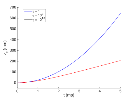
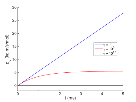
   Figure 1: (Color online) Plots of the center of the position (up) and momentum (down) PDFs, as given by Eqs. (16) (17), respectively, for three values of the parameter $\gamma$.

   

   

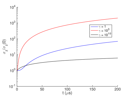
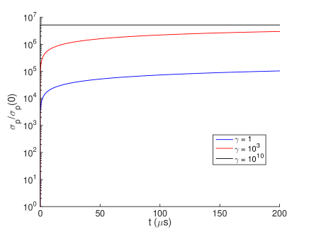
   Figure 2: (Color online) Plots of the width of the position (up) and momentum (down) PDFs, for three values of the parameter $\gamma$.

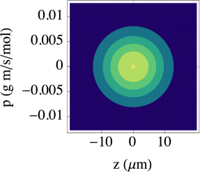
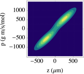
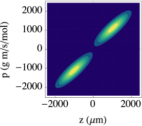
Figure 3: (Color online) Contour plots of the trace of the matrix Wigner function with $\gamma=1$ s^-1. The left panel corresponds to the initial ($t=0)$ state, while the middle panel shows the situation at $t=100\,\,\mu s$, and the right panel is for $t=200\,\,\mu s$.

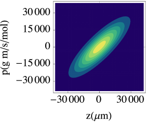
Figure 4: (Color online) Same as Fig. 3, for a value $\gamma=10^{3}$ s^-1.

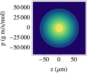
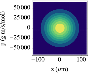
Figure 5: (Color online) Same as Fig. 3, using $\gamma=10^{10}$ s^-1.

III Application to the Stern-Gerlach experiment

The study of a realistic SG experiment setup with decoherence effects will be the core of this section. First, parameters for the setup will be introduced. Then, the evolution of the system will be pictured in phase space using the results from the previous section. To conclude, the characteristic decoherence time of the system will be studied through the damping of the off-diagonal elements of the Wigner function as the system evolves.

III.1 Experiment parameters

We assume an incident beam of Silver atoms ($m=1.8\times 10^{-25}$ kg, $g_{s}\simeq 2$) starting in the $\left|S_{x}=\hbar/2\right\rangle=\frac{1}{\sqrt{2}}\left|+\right\rangle+\frac{1}{\sqrt{2}}\left|-\right\rangle$ spin state, with an average speed $v=500$ m/s, and a beam width $\sigma=10^{-5}$ m. The SG apparatus parameters are based on the realistic ones used in a previous work Gondran and Gondran (2013). In this setup, the applied magnetic field is $B_{0}=5$ T, and the gradient $\eta=1000$ T/m. The longitude of the tube is $l=0.2$ m, which implies a flight time of around $0.4$ ms for the above Silver atoms speed. This is, therefore, the characteristic time scale for the system dynamics. The operational temperature of the tube is around $T\simeq 300$ K, i.e. the laboratory temperature.

III.2 Phase space representation

In this section we will illustrate the behavior of the SG experiment in a decoherent environment, by showing some plots of the Wigner function using the parameters defined in Sect. III.1.

III.2.1 Diagonal elements

In order to represent the phase space distribution of the particle, the trace of the matrix Wigner function is plotted for $\gamma=1,\ 10^{3},\ 10^{10}$ s^-1 in Figures 3, 4 and 5, respectively. The trace allows us to show the total quasi-probability distribution, thus putting on the same plot both spin components. Fig. 3 ($\gamma=1$ s^-1) shows how the incoming state splits into two separating components within the experiment timescale ($<$ 1 ms): At $t=100\,\,\mu s$ both terms start to split, and at $t=200\,\,\mu s$ they are visibly separated. We observe the distortion of the original shape of the Wigner function, caused by the different evolution in $z$ and $p$, that appears even when the interaction with the environment is not included (see Utz et al. (2015)). Note also that friction with the environment quickly broadens the spatial width, from the initial value to the millimeter scale in just $t=200\,\,\mu s$. The same behavior can be observed for the momentum width.

As can be seen in Fig. 4 ($\gamma=10^{3}$ s^-1), a higher value of the friction force quickly limits the momentum of the peak centers, and causes the growth of the distribution widths. The influence of the SG apparatus is still visible in the shape of the beam, but due to the speed limit and the continuous growth of the width, the two components of the beam do not separate. An even larger value of the friction force (Fig. 5) causes the distribution peak centers to remain at the origin, and the width of the momentum distribution quickly grows, thus completely masking all the effects of the apparatus.

III.2.2 Off-diagonal elements

To study the off-diagonal Wigner function, two 3D-plots of the real part of $W_{od}(z,p,t)$, corresponding to $\gamma=1,\ 10^{10}$ s^-1, are drawn in order to see how the value of the damping constant affects the decoherence rate. At $t=0$ (Fig. 6) this amounts to representing the initial Gaussian distribution Eq. (14).

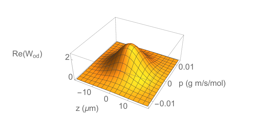
Figure 6: (Color online) 3D-plot of the real part of $W_{od}(z,p,t)$ at $t=0$.

As time goes on, Figs. 7 and 8 show how the real part of $W_{od}(z,p,\tau)$ evolves, from a Gaussian distribution, to an oscillatory function. We also observe that these oscillations are damped due to the interaction with the environment. By comparing both figures, we immediately see that a larger value of $\gamma$ increases the oscillation frequency and reduces the amplitude of the oscillations, thus leading to a faster decoherence.

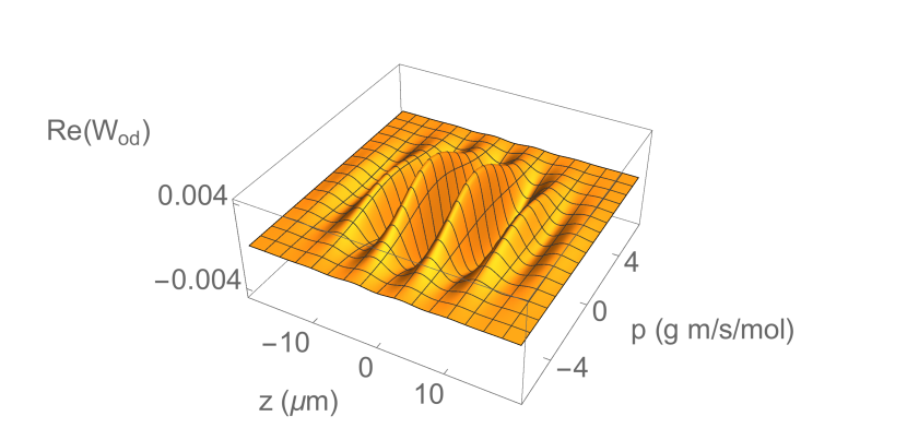
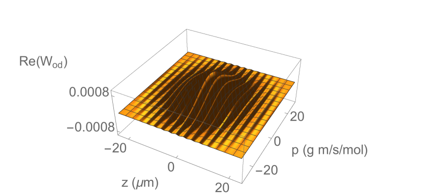
Figure 7: (Color online) 3D-plot of the real part of $W_{od}(z,p,t)$ at $t=0.005\mu s$ (up) and $t=0.1\mu s$ (down), for $\gamma=1$ s^-1.

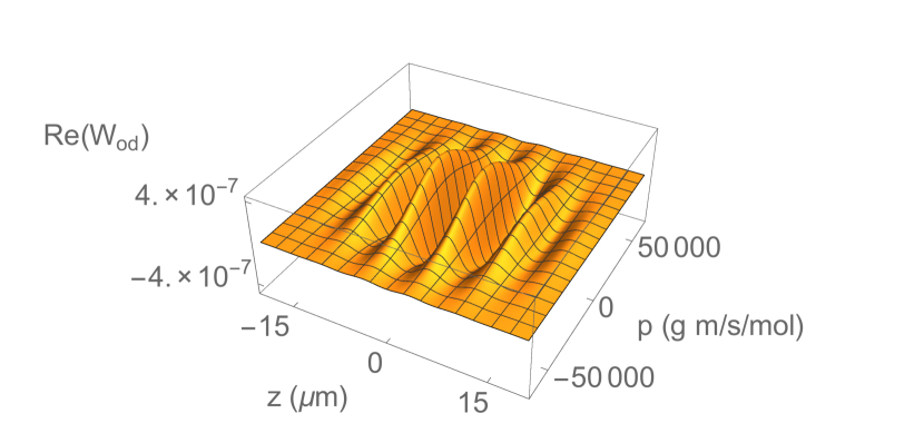
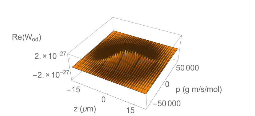
Figure 8: (Color online) Same as Fig. 7, for $\gamma=10^{10}$ s^-1.

III.3 Decoherence time

In order to quantify the loss of coherence in the system we choose, as a figure of merit, the norm $\Delta(t)$ of $W_{od}(z,p,t)$ at a given $t$, defined as

$$\Delta(t)\equiv\int_{-\infty}^{\infty}\int_{-\infty}^{\infty}|W_{od}(z,p,t)|\,\,dz\,\,dp.$$ (30)

This quantity provides the total volume, in phase space, occupied by the coherent term of the Wigner function. Taking the module, instead of the function itself, avoids for cancellations due to the oscillatory nature of this term. In Fig. 9 we have plotted $\Delta(t)$ for different values of $\gamma$. As expected, decoherence effects manifest in a decrease of $\Delta(t)$ with time. In fact, the approach to zero appears at earlier times as one considers larger values of $\gamma$, clearly indicating a faster decoherence process.

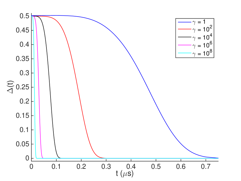
Figure 9: (Color online) Plot of $\Delta(t)$, as defined by Eq. (30), for different values $\gamma=1,10^{2},10^{4},10^{6},10^{8}$ s^-1, as a function of time.

In view of this result, we can introduce a decoherence time $t_{d}$, as the time it takes for $\Delta(t)$ to reduce its initial value by a factor $e$. From the above data, we can obtain $t_{d}$ for a given value of $\gamma$. These data are collected in Fig. 10.

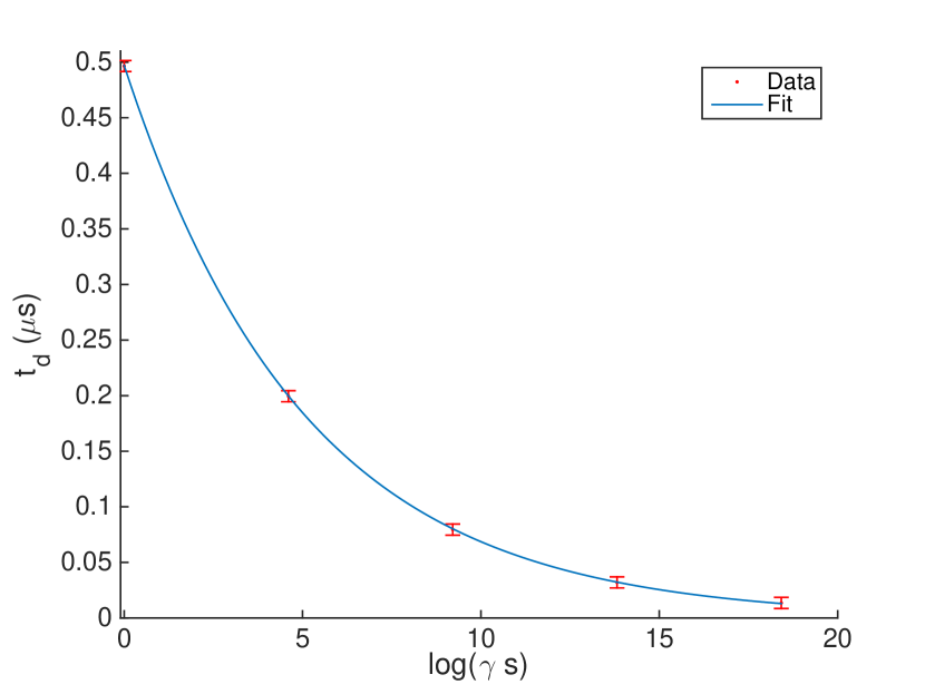
Figure 10: (Color online) Red points show the decoherence time $t_{d}$ for the same values of $\gamma$ used in Fig. (9). The bar indicates the imprecision that originates from the data. The solid curve is our fit $t_{d}=a\ \gamma^{b}$ (see the text for explanation).

Performing a numerical fit to the curve $t_{d}(\gamma)$ we find that the decoherence time can be approximated by the formula $t_{d}=a\ \gamma^{b}$, with $a=0.497\pm 0.002$ and $b=-0.198\pm 0.001$, pointing to a behavior as $t_{d}\propto\gamma^{-1/5}$. This result is at variance with the one discussed in Venugopalan et al. (1995), where a decoherence time given by $\left(\frac{3\hbar^{2}m^{2}\gamma^{2}}{4D\eta^{2}\lambda^{2}}\right)^{1/3}$ was claimed, which translates into a dependence of the form $t_{d}\propto\gamma^{1/3}$, i.e. the larger the decoherence parameter $\gamma$, the later the system experiences decoherence. In our opinion, such result is unrealistic, as one expects the opposite behavior: Decoherence should take place faster as $\gamma$ is increased, in accordance to our results.

III.4 Discussion about the validity of the model

In the SG experiment, Silver atoms travel through the high vacuum beam pipe. We assume that they collide with the residual air molecules, resulting into Brownian motion and decoherence. In the Caldeira-Leggett master equation, these effects are included via the damping rate $\gamma$. The Langevin equation relates $\gamma$ to the viscosity $\mu$ as follows Zurek (2002)

$$\gamma=\frac{\mu}{2m},$$ (31)

with $\mu$ the viscosity of the medium for Silver atoms. This quantity can be explicitly calculated through the following expression Marquardt (1999)

$$\mu=6\pi R\mu^{\prime}=2.994\ \pi RnM_{M}v_{M}\lambda_{M},$$ (32)

where $R=144$ pm is the radius of the Silver atom, $n$ is the particle number density of the air; $M_{M}$, $v_{M}$ and $\lambda_{M}$ are the molecular mass, mean speed and mean free path of air molecules, respectively. The Stokes’ law term $6\pi R$ accounts for the contribution of Silver atoms mass to the viscosity Batchelor and Young (1968), and the term $\mu^{\prime}=0.499\ nM_{M}v_{M}\lambda_{M}$ accounts for the air contribution. Assuming typical values for the pressure of the beam pipe $P\simeq 10^{-6}$ mbar PHYWE , one finds Marquardt (1999) $n\simeq 10^{10}$ cm^-3, $\lambda_{M}\simeq 10^{4}$ cm, and $v_{M}\simeq 500$ m/s. To obtain a rough estimate, we assume that the molecules in the low pressure conditions in the tube are mostly composed by $N_{2}$, with a mass $M_{M}\simeq 28$ uma $=4.65\ 10^{-26}$ kg.

Using the above data, one obtains the estimate $\mu\sim 10^{-14}$ Kg/s, implying that the order of magnitude of $\gamma$ is $\sim 10^{10}$ s^-1. Such value, however, posses a problem: As we have seen (Fig. 4), for damping rates larger than $10^{3}$ s^-1, the two components of the initial state do not separate due to the high friction with the environment. This is obviously not what happens in the real experiment, leading us to serious doubts of the application of the Caldeira-Leggett model to the SG experiment.

A possible explanation of this disagreement might be that the obtained value of $\gamma$ is wrong, because the calculation of the viscosity discussed above is not correct in high vacuum. As Marquardt (1999) indicates, when $\lambda_{M}$ is larger than the size of the container, the gas is in a molecular state, and cannot be characterized by a viscosity anymore. Furthermore, as explained in PHYWE , due to the high vacuum in the beam pipe, the mean free path of Silver atoms is a multiple of the beam pipe length. Under these conditions, one should question the validity of the master equation Eq. (3), which was used to derive the corresponding differential equations that describe the Wigner function dynamics.

IV Conclusions

In this paper, we have studied the SG experiment with environmental induced decoherence described by the Caldeira-Leggett model. Our description is done on the phase space, making use of Wigner functions, with the additional spin degree of freedom. Our goal was to describe the kinematics of the atoms traversing the magnetic field gradient, and interacting with a thermal bath of particles, leading to Brownian motion and decoherence. We solved the differential equations for the Wigner function corresponding to the model, starting from an initial separable state, with a Gaussian shape in space, and an arbitrary spin state. The diagonal terms on the $S_{z}$ basis have a simple interpretation, in terms of the two separating states of the apparatus. By calculating the marginals over momentum or position for each of the diagonal terms of the Wigner function, we obtain the probability distribution for the conjugate variable. Each of the obtained diagonal distributions conserve the initial Gaussian shape, both in position and in space, in spite of the interaction with the environment, and allow for a clear description in terms of the center and width of the corresponding Gaussian, which bear a close analogy with the classical Brownian motion of a particle. In particular, at large times the particle reaches a limit velocity, a feature which is particularly important for the description of the SG experiment inside a gas tube. We also showed that our results agree with the non decoherence expressions in the appropriate limit.

By adopting realistic parameters for the SG experiment, we plotted the diagonal and off-diagonal elements of the Wigner function. We observe that, for low values of the decoherence parameter $\gamma$, the initial state separates into two components, corresponding to the up and down spin, as expected. The off-diagonal terms provide us information about decoherence, as a consequence of the interaction with the environment, that manifests in the damping of these terms as time evolves. In order to quantify the effect of decoherence, we evaluate the norm of the off-diagonal element over the whole phase space. The characteristic decoherence time scale $t_{d}$ is defined as the instant when the initial norm is reduced by a factor $e$. By obtaining $t_{d}$ for different values of $\gamma$, we find a relation which is well described by a power law $t_{d}\propto\gamma^{-1/5}$. Our result differs from previous results, where a dependence $t_{d}\propto\gamma^{1/3}$ was claimed instead. We argue that such dependence is counter intuitive, as it would imply that a larger value of $\gamma$ makes decoherence effects to appear later. In contrast, we obtain that a stronger value of $\gamma$ implies a shorter decoherence time, which seems more reasonable.

Finally, we discuss a caveat of the model, that shows up after estimating the order of magnitude of $\gamma$ in a realistic scenario. In fact, we obtain $\gamma\sim 10^{10}$, a value that would lead to a large friction, and would ruin the observed phenomenology of the experiment. This estimate has itself a loophole, as the calculated mean free path of the incoming particles on the tube turns out to be of the order of the tube length, thus implying that collisions with the air molecules are rare events. Altogether, these reasonings rise some doubts on the applicability of the Caldeira-Leggett model for this problem. In our opinion, this question deserves further research, given the importance of the experiment as one of the cornerstones in quantum physics.

V Auxiliary formulae for the diagonal and off-diagonal Wigner function

In this Appendix, we give the explicit expressions for auxiliary functions that define both the diagonal and off-diagonal terms of the matrix WF. The functions $F(z,p,\tau)$ and $G(\tau)$ that enter in the diagonal part Eq. (15) are defined as

$$F(z,p,\tau) = 2\gamma D\sigma^{2}\left[\left(\gamma^{2}m^{2}\left(1-e^{-2\tau}\right)z^{\prime 2}-2\gamma mp^{\prime}\left(1-e^{-\tau}\right)^{2}z^{\prime}+p^{\prime 2}\left(-\left(2-e^{-\tau}\right)^{2}+2\tau+1\right)\right)\right.$$ (33)

$$+ \left.\gamma^{4}m^{2}p^{\prime 2}\sigma^{4}+\gamma^{2}\hbar^{2}\left(p^{\prime}\left(1-e^{-\tau}\right)-\gamma me^{-\tau}z^{\prime}\right)^{2}\right],$$

$$G(\tau) = 8D^{2}\sigma^{2}\left(1-e^{-\tau}\right)\left(\left(e^{-\tau}+1\right)\tau-2\left(1-e^{-\tau}\right)\right)+2\gamma D\left[\gamma^{2}m^{2}\sigma^{4}\left(1-e^{-2\tau}\right)\right.$$ (34)

$$+ \left.\left(e^{-2\tau}(2\tau+3)-4e^{-\tau}+1\right)\hbar^{2}\right]+\gamma^{4}m^{2}\sigma^{2}e^{-2\tau}\hbar^{2},$$

where $z^{\prime}=z\mp z_{c}$, $p^{\prime}=p\mp p_{c}$. The magnitudes $z_{c}$ and $p_{c}$ are given in Eqs. (16) and (17), respectively.

For the off diagonal term defined in Eq. (18) we introduced the following definitions:

$$C_{1}(\tau)=\frac{\eta^{2}\lambda^{2}\left(\sigma^{2}\left(-2D\left(2\tau^{3}-6\tau^{2}+6\tau+3\right)+6De^{-2\tau}+24De^{-\tau}\tau-3\gamma^{3}m^{2}\sigma^{2}\tau^{2}\right)-3\gamma\left(1-\tau-e^{-\tau}\right)^{2}\hbar^{2}\right)}{3\gamma^{5}m^{2}\sigma^{2}\hbar^{2}},$$ (35)

$$C_{2}(\tau)=\frac{\eta\lambda\left(\gamma\hbar^{2}\left(e^{-\tau}-e^{-\tau}\tau-e^{-2\tau}\right)-2D\sigma^{2}\left(1-2e^{-\tau}\tau-e^{-2\tau}\right)\right)}{\gamma^{3}\hbar^{2}m\sigma^{2}},$$ (36)

$$C_{3}(\tau)=\frac{\sigma^{2}\left(2De^{-2\tau}-8De^{-\tau}-D(4\tau-6)-\gamma^{3}m^{2}\sigma^{2}\right)-\gamma\hbar^{2}\left(1-e^{-\tau}\right)^{2}}{4\gamma^{3}m^{2}\sigma^{2}},$$ (37)

$$C_{4}(\tau)=\frac{\eta\lambda\left(\gamma\left(1-e^{-\tau}\right)\left(1-\tau-e^{-\tau}\right)\hbar^{2}-\sigma^{2}\left(2D\left(\tau+e^{-\tau}-1\right)^{2}+\gamma^{3}m^{2}\sigma^{2}\tau\right)\right)}{\gamma^{4}m^{2}\sigma^{2}\hbar},$$ (38)

$$C_{5}(\tau)=\frac{\left(e^{-\tau}-1\right)\left(\gamma e^{-\tau}\hbar^{2}+2D\sigma^{2}\left(1-e^{-\tau}\right)\right)}{2\gamma^{2}m\sigma^{2}\hbar},$$ (39)

$$C_{6}(\tau)=\frac{\gamma e^{-2\tau}\hbar^{2}+2D\sigma^{2}\left(1-e^{-2\tau}\right)}{4\gamma\sigma^{2}\hbar^{2}}.$$ (40)

References

- Gerlach and Stern (1922) W. Gerlach and O. Stern, Zeitschrift für Physik 9, 349 (1922).
- Reinisch (1999) G. Reinisch, Physics Letters A 259, 427 (1999).
- Cruz-Barrios et al. (2003) S. Cruz-Barrios, M. C. Nemes, and A. F. R. de Toledo Piza, Europhysics Letters 61, 148 (2003), arXiv:cond-mat/0202055 .
- Tumminello et al. (2005) M. Tumminello, A. Vaglica, and G. Vetri, European Physical Journal D 36, 235 (2005), arXiv:quant-ph/0503033 .
- van Huele et al. (2010) J.-F. S. van Huele, B. C. Hsu, and J. R. Stenson, in APS Meeting Abstracts (2010) p. 42010.
- Roston et al. (2005) G. B. Roston, M. Casas, A. Plastino, and A. R. Plastino, European Journal of Physics 26, 657 (2005).
- Caldeira and Leggett (1981) A. O. Caldeira and A. J. Leggett, Phys. Rev. Lett. 46, 211 (1981).
- Venugopalan et al. (1995) A. Venugopalan, D. Kumar, and R. Ghosh, Physica A Statistical Mechanics and its Applications 220, 563 (1995).
- Wigner (1932) E. Wigner, Phys. Rev. 40, 749 (1932).
- Lee et al. (2011) N. Lee, H. Benichi, Y. Takeno, S. Takeda, J. Webb, E. Huntington, and A. Furusawa, Science 332, 330 (2011).
- Dahl et al. (2006) J. P. Dahl, H. Mack, A. Wolf, and W. P. Schleich, Phys. Rev. A 74, 042323 (2006).
- Hillery et al. (1984) M. Hillery, R. F. O’Connell, M. O. Scully, and E. P. Wigner, Physics Reports 106, 121 (1984).
- Wallentowitz et al. (1997) S. Wallentowitz, R. L. de Matos Filho, and W. Vogel, Phys. Rev. A 56, 1205 (1997).
- Utz et al. (2015) M. Utz, M. H. Levitt, N. Cooper, and H. Ulbricht, Phys. Chem. Chem. Phys. 17, 3867 (2015).
- Massini et al. (2000) M. Massini, M. Fortunato, S. Mancini, P. Tombesi, and D. Vitali, New Journal of Physics 2, 20 (2000).
- Schleich (2001) W. P. Schleich, Quantum Optics in Phase Space, 1st ed. (Wiley-VCH, 2001).
- Platt (1992) D. E. Platt, American Journal of Physics 60, 306 (1992).
- Breuer and Petruccione (2007) H.-P. Breuer and F. Petruccione, The Theory of Open Quantum Systems (Oxford University Press, Oxford, 2007).
- Gondran and Gondran (2013) M. Gondran and A. Gondran, , 15 (2013), arXiv:1309.4757 .
- Zurek (2002) W. H. Zurek, Los Alamos Science (2002), arXiv:0306072 .
- Marquardt (1999) N. Marquardt, Vacuum , 1 (1999).
- Batchelor and Young (1968) G. K. Batchelor and A. D. Young, Journal of Applied Mechanics 35, 624 (1968), arXiv:9780471202318 .
- (23) PHYWE, “Stern Gerlach apparatus manual,” .