Structure formation and generalized second law of thermodynamics in some viable $f(R)$-gravity models

Abstract

Here, we investigate the growth of matter density perturbations as well as the generalized second law (GSL) of thermodynamics in the framework of $f(R)$-gravity. We consider a spatially flat FRW universe filled with the pressureless matter and radiation which is enclosed by the dynamical apparent horizon with the Hawking temperature. For some viable $f(R)$ models containing the Starobinsky, Hu-Sawicki, Exponential, Tsujikawa and AB models, we first explore numerically the evolution of some cosmological parameters like the Hubble parameter, the Ricci scalar, the deceleration parameter, the density parameters and the equation of state parameters. Then, we examine the validity of GSL and obtain the growth factor of structure formation. We find that for the aforementioned models, the GSL is satisfied from the early times to the present epoch. But in the farther future, the GSL for the all models is violated. Our numerical results also show that for the all models, the growth factor for larger structures like the $\Lambda$CDM model fit the data very well.

I Introduction

The observed accelerated expansion of the universe, as evidenced by a host of cosmological data such as supernovae Ia (SNeIa) SNeIa , cosmic microwave background (CMB) WMAP ; Planck , large scale structure (LSS) LSS , etc., came as a great surprise to cosmologists. The present accelerated phase of the universe expansion reveals new physics missing from our universe’s picture, and it constitutes the fundamental key to understand the fate of the universe.

There are two representative approaches to explain the current acceleration of the universe. One is to introduce “dark energy” (DE) Padmanabhan in the framework of general relativity (GR). The other is to consider a theory of modified gravity (MG), such as $f(R)$ gravity, in which the Einstein-Hilbert action in GR is generalized from the Ricci scalar $R$ to an arbitrary function of the Ricci scalar Sotiriou1 . Here, we will focus on the later approach.

In Sotiriou2 , it was shown that a $f(R)$ model with negative and positive powers of Ricci curvature scalar $R$ can naturally combine the inflation at early times and the cosmic acceleration at late times. It is actually possible for viable $f(R)$ models for late time acceleration to include inflation by adding $R^{2}$ term. Therefore, it is natural to consider combined $f(R)$ models which describe both primordial and present DE using one $f(R)$ function, albeit one containing two greatly different characteristic energy scales AB ; Motohashi . In Sobouti , it was pointed out that the $f(R)$-gravity can also serve as dark matter (DM). In Khaledian , a set of $f(R)$-gravity models corresponding to different DE models were reconstructed. Although a great variety of $f(R)$ models have been proposed in the literature, most of them is not perfect enough. An interesting feature of the $f(R)$ theories is the fact that the gravitational constant in $f(R)$-gravity, varies with length scale as well as with time Raccanelli -deltam . Thus the evolution of the matter density perturbation, $\delta_{\rm m}\equiv\delta\rho_{\rm m}/\rho_{\rm m}$, in this theory is affected by the effective Newton coupling constant, $G_{\rm eff}$, and it is scale dependent too. Therefore, the matter density perturbation is a crucial tool to distinguish MG from DE model in GR, in particular the standard $\Lambda$CDM model.

On the other hand, the connection between gravity and thermodynamics is one of surprising features of gravity which was first reinforced by Jacobson Jacobson , who associated the Einstein field equations with the Clausius relation in the context of black hole thermodynamics. This idea was also extended to the cosmological context and it was shown that the Friedmann equations in the Einstein gravity Cai05 can be written in the form of the first law of thermodynamics (the Clausius relation). The equivalence between the first law of thermodynamics and the Friedmann equation was also found for $f(R)$-gravity Akbar12 . Besides the first law, the generalized second law (GSL) of gravitational thermodynamics, which states that entropy of the fluid inside the horizon plus the geometric entropy do not decrease with time, was also investigated in $f(R)$-gravity kka1 . The GSL of thermodynamics in the accelerating universe driven by DE or MG has been also studied extensively in the literature Izquierdo1 -Geng .

All mentioned in above motivate us to investigate the growth of matter density perturbations in a class of metric $f(R)$ models and see scale dependence of growth factor. Additionally, we are interested in examining the validity of GSL in some viable $f(R)$-gravity models. The structure of this paper is as follows. In Sec. II, within the framework of $f(R)$-gravity we consider a spatially flat Friedmann-Robertson-Walker (FRW) universe filled with the pressureless matter and radiation. In Sec. III, we study the growth rate of matter density perturbations in $f(R)$-gravity. In Sec. IV, the GSL of thermodynamics on the dynamical apparent horizon with the Hawking temperature is explained. In Sec. V, the cosmological evolution of $f(R)$ models is illustrated. In Sec. VI, the viability conditions for $f(R)$ models are discussed. In addition, some viable $f(R)$ models containing the Starobinsky, Hu-Sawicki, Exponential, Tsujikawa and AB models are introduced. In Sec. VII, we give numerical results obtained for the evolution of some cosmological parameters, the GSL and the growth of structure formation in the aforementioned $f(R)$ models. Section VIII is devoted to conclusions.

II $f(R)$-gravity framework

Within the framework of $f(R)$-gravity, the modified Einstein-Hilbert action in the Jordan frame is given by Sotiriou1

$$S_{\rm J}=\int{\sqrt{-g}}~{}{\rm d}^{4}x\left[\frac{{f(R)}}{{16\pi G}}+L_{\rm matter}\right],$$ (1)

where $G$, $g$, $R$ and $L_{\rm matter}$ are the gravitational constant, the determinant of the metric $g_{\mu\nu}$, the Ricci scalar and the lagrangian density of the matter inside the universe, respectively. Also $f(R)$ is an arbitrary function of the Ricci scalar.

Varying the action (1) with respect to $g_{\mu\nu}$ yields

$$FG_{\mu\nu}=8\pi GT^{(\rm m)}_{\mu\nu}-\frac{1}{2}g_{\mu\nu}(RF-f)+\nabla_{\mu}\nabla_{\nu}F-g_{\mu\nu}\square F.$$ (2)

Here $F={\rm d}f/{\rm d}R$, $G_{\mu\nu}=R_{\mu\nu}-\frac{1}{2}Rg_{\mu\nu}$ and $T^{(\rm m)}_{\mu\nu}$ is the energy-momentum tensor of the matter. The gravitational field equations (2) can be rewritten in the standard form as action ; TX

$$G_{\mu\nu}=8\pi G\big{(}T^{(\rm m)}_{\mu\nu}+T^{(\rm D)}_{\mu\nu}\big{)},$$ (3)

with

$$8\pi GT^{(\rm D)}_{\mu\nu}=(1-F)G_{\mu\nu}-\frac{1}{2}g_{\mu\nu}(RF-f)+\nabla_{\mu}\nabla_{\nu}F-g_{\mu\nu}\square F.$$ (4)

For a spatially flat FRW metric, taking $T_{\nu}^{\mu(m)}={\rm diag}(-\rho,p,p,p)$ in the prefect fluid form, then the set of field equations (3) reduce to the modified Friedmann equations in the framework of $f(R)$-gravity as Capozziello2

$$3H^{2} = 8\pi G(\rho+\rho_{\rm D}),$$ (5)

$$2\dot{H} = -8\pi G(\rho+\rho_{\rm D}+p+p_{\rm D}),$$ (6)

where

$$8\pi G\rho_{\rm D} = \frac{1}{2}\big{(}RF-f\big{)}-3H\dot{F}+3H^{2}\big{(}1-F\big{)},$$ (7)

$$8\pi Gp_{\rm D} = \left[\frac{-1}{2}\big{(}RF-f\big{)}+\ddot{F}+2H\dot{F}-(1-F)\big{(}2\dot{H}+3H^{2}\big{)}\right],$$ (8)

with

$$R=6(\dot{H}+2H^{2}).$$ (9)

Here $H=\dot{a}/a$ is the Hubble parameter. Also $\rho_{\rm D}$ and $p_{\rm D}$ are the curvature contribution to the energy density and pressure which can play the role of DE. Also $\rho=\rho_{\rm BM}+\rho_{\rm DM}+\rho_{\rm rad}$ and $p=p_{\rm rad}=\rho_{\rm rad}/3$ are the energy density and pressure of the matter inside the universe, consist of the pressureless baryonic and dark matters as well as the radiation. On the whole of the paper, the dot and the subscript $R$ denote the derivatives with respect to the cosmic time $t$ and the Ricci scalar $R$, respectively.

The energy conservation laws are still given by

$$\dot{\rho}_{\rm m}+3H\rho_{\rm m}=0,$$ (10)

$$\dot{\rho}_{\rm rad}+4H\rho_{\rm rad}=0,$$ (11)

$$\dot{\rho}_{\rm D}+3H(\rho_{\rm D}+p_{\rm D})=0,$$ (12)

where $\rho_{\rm m}=\rho_{\rm BM}+\rho_{\rm DM}$. From Eqs. (10) and (11) one can find

$$\rho=\frac{\rho_{\rm m_{0}}}{a^{3}}+\frac{\rho_{\rm rad_{0}}}{a^{4}},$$ (13)

where $\rho_{\rm m_{0}}=\rho_{\rm BM_{0}}+\rho_{\rm DM_{0}}$ and $\rho_{\rm rad_{0}}$ are the present values of the energy densities of matter and radiation. We also choose $a_{0}=1$ for the recent value of the scale factor.

Using the usual definitions of the density parameters

$$\Omega_{\rm m}=\frac{\rho_{\rm m}}{\rho_{\rm c}}=\frac{8\pi G\rho_{\rm m_{0}}}{3H^{2}a^{3}},~{}~{}~{}\Omega_{\rm rad}=\frac{\rho_{\rm rad}}{\rho_{\rm c}}=\frac{8\pi G\rho_{\rm rad_{0}}}{3H^{2}a^{4}},~{}~{}~{}\Omega_{\rm D}=\frac{\rho_{\rm D}}{\rho_{\rm c}}=\frac{8\pi G\rho_{\rm D}}{3H^{2}},$$ (14)

in which $\rho_{\rm c}=3H^{2}/(8\pi G)$ is the critical energy density, the modified Friedmann equation (5) takes the form

$$1=\Omega_{\rm m}+\Omega_{\rm rad}+\Omega_{\rm D}.$$ (15)

From the energy conservation (12), the equation of state (EoS) parameter due to the curvature contribution is defined as

$$\omega_{\rm D}=\frac{p_{\rm D}}{\rho_{\rm D}}=-1-\frac{\dot{\rho}_{\rm D}}{3H\rho_{\rm D}}.$$ (16)

Using the modified Friedmann equations (5) and (6), the effective EoS parameter is obtained as

$$\omega_{\rm eff}=\frac{p+p_{\rm D}}{\rho+\rho_{\rm D}}=-1-\frac{2\dot{H}}{3H^{2}}.$$ (17)

Also the two important observational cosmographic parameters called the deceleration $q$ and the jerk $j$ parameters, respectively related to $\ddot{a}$ and $\dddot{a}$, are given by cosmography

$$q = -\frac{\ddot{a}}{aH^{2}}=-1-\frac{\dot{H}}{H^{2}}=1-\frac{R}{6H^{2}},$$ (18)

$$j = \frac{\dddot{a}}{aH^{3}}=1-\frac{\dot{H}}{H^{2}}+\frac{\dot{R}}{6H^{3}}=2+q+\frac{\dot{R}}{6H^{3}}.$$ (19)

III Growth rate of matter density perturbations

Here, we study the evolution of the matter density contrast $\delta_{\rm m}=\delta\rho_{\rm m}/\rho_{\rm m}$ in $f(R)$-gravity. To this aim, we consider the linear scalar perturbations around a flat FRW background in the Newtonian (longitudinal) gauge as

$${\rm d}s^{2}=-(1+2\Psi){\rm d}t^{2}+a^{2}(t)(1+2\Phi){\rm d}x^{2},$$ (20)

with two scalar potentials $\Psi$ and $\Phi$ describing the perturbations in the metric. In this gauge, the matter density perturbation $\delta_{\rm m}$ and the perturbation of $\delta F(R)$ obey the following equations in the Fourier space Hwang ; Tsujik

$$\ddot{\delta}_{\rm m}+\left(2H+\frac{\dot{F}}{2F}\right)\dot{\delta}_{\rm m}-\frac{8\pi G\rho_{\rm m}}{2F}\delta_{\rm m}=\frac{1}{2F}\left[\left(-6H^{2}+\frac{k^{2}}{a^{2}}\right)\delta F+3H\dot{\delta F}+3\ddot{\delta F}\right],$$ (21)

$$\ddot{\delta F}+3H\dot{\delta F}+\left(\frac{k^{2}}{a^{2}}+\frac{F}{3F_{\rm R}}-\frac{R}{3}\right)\delta F=\frac{8\pi G}{3}\rho_{\rm m}\delta_{\rm m}+\dot{F}\dot{\delta}_{\rm m},$$ (22)

where $k$ is the comoving wave number. For the modes deep inside the Hubble radius (i.e. $k^{2}/a^{2}\gg H^{2}$), we have $|\dot{F}|\ll HF$ and $\ddot{\delta F}\ll H\dot{\delta F}\ll H^{2}$, hence the evolution of matter density contrast $\delta_{\rm m}$ reads Starobinsky ; Tsu

$$\ddot{\delta}_{\rm m}+2H\dot{\delta}_{\rm m}-4\pi G_{\rm eff}\rho_{\rm m}\delta_{\rm m}=0,$$ (23)

where

$$G_{\rm eff}=\frac{G}{F}\left[\frac{4}{3}-\frac{1}{3}\frac{M^{2}a^{2}}{k^{2}+M^{2}a^{2}}\right],$$ (24)

and $M^{2}=\frac{F}{3F_{\rm R}}$. The fraction of effective gravitational constant to the Newtonian one, i.e. $G_{\rm eff}/G$, is defined as screened mass function in the literature Rahvar . Equation (24) obviously shows that the screened mass function is the time and scale dependent parameter.

With the help of new variable namely $g(a)=\delta_{\rm m}/a$ which parameterizes the growth of structure in the matter, Eq. (23) becomes

$$\frac{{\rm d}^{2}g}{{\rm d}\ln{a^{2}}}+\left(4+\frac{\dot{H}}{{H}^{2}}\right)\frac{{\rm d}g}{{\rm d}\ln{a}}+\left(3+\frac{\dot{H}}{{H}^{2}}-\frac{4{\pi}G_{\rm eff}\rho_{\rm m}}{H^{2}}\right)g=0.$$ (25)

In general, there is no analytical solution to this equation. But in Yokoyama for an asymptotic form of viable $f(R)$ models at high curvature regime given by $f(R)=R+R^{-n}$ where $n>-1$, an analytic solution for density perturbations in the matter component during the matter dominated stage was obtained in terms of hypergeometric functions. In what follows we solve the differential equation (25), numerically. To this aim, the natural choice for the initial conditions are $g(a_{\rm m})=1$ and $\frac{\rm dg}{\rm d\ln a}\mid_{a=a_{\rm m}}=0$, where $a_{\rm m}=1/(1+z_{\rm m})$ should be taken during the matter era, because for the matter dominated universe, i.e. $H^{2}=8\pi G\rho_{\rm m}/3$ and $G_{\rm eff}/G=1$, the solution of Eq. (23) yields $\delta_{\rm m}=a$. The growth factor is defined as Peebles

$$f(z)=\frac{{\rm d}\ln\delta_{\rm m}}{{\rm d}\ln a}=-(1+z)\,\frac{{\rm d}\ln\delta_{\rm m}}{{\rm d}z},$$ (26)

which is an observational parameter. In the present work, we obtain the evolution of linear perturbations relevant to the matter spectrum for the scales; $k=0.1,0.01,0.001$ $h~{}{\rm Mpc}^{-1}$, where $h$ corresponds to the Hubble parameter today.

IV Generalized second law of thermodynamics

Here, we are interested in examining the validity of the GSL of gravitational thermodynamics for a given $f(R)$ model. According to the GSL, entropy of the matter inside the horizon beside the entropy associated with the surface of horizon should not decrease during the time Cai05 . As demonstrated by Bekenstein, this law is satisfied by black holes in contact with their radiation Bekenstein . The entropy of the matter containing the pressureless matter and radiation inside the horizon is given by the Gibbs’ equation Izquierdo1

$$T_{\rm A}{\rm d}S={\rm d}E+p{\rm d}V.$$ (27)

Taking time derivative of Eq. (27) and using the energy equations (10)-(11) as well as the Friedmann equations (5)-(6) one can find

$$T_{\rm A}\dot{S}=\frac{\tilde{r}^{2}_{\rm A}}{2G}\left(\dot{\tilde{r}}_{\rm A}-H\tilde{r}_{\rm A}\right)\left(-2\dot{H}+H\frac{{\rm d}}{{\rm d}t}-\frac{{\rm d}^{2}}{{\rm d}t^{2}}\right)F,$$ (28)

where $\tilde{r}_{\rm A}=(H^{2}+\frac{K}{a^{2}})^{-1/2}$ and $T_{\rm A}=\frac{1}{2\pi\tilde{r}_{\rm A}}\big{(}1-\frac{\dot{\tilde{r}}_{\rm A}}{2H\tilde{r}_{\rm A}}\big{)}$ are the dynamical apparent horizon and Hawking temperature, respectively. The horizon entropy in $f(R)$-gravity is given by $S_{\rm A}=\frac{AF}{4G}$ Wald , where $A=4\pi\tilde{r}^{2}_{\rm A}$ is the area of the apparent horizon. Taking the time derivative of $S_{\rm A}$ one can get the evolution of horizon entropy as

$$T_{\rm A}\dot{S}_{\rm A}=\frac{1}{4GH}\left(2H\tilde{r}_{\rm A}-\dot{\tilde{r}}_{\rm A}\right)\left(\frac{2\dot{\tilde{r}}_{\rm A}}{\tilde{r}_{\rm A}}+\frac{{\rm d}}{{\rm d}t}\right)F.$$ (29)

Now we can calculate the GSL due to different contributions of the matter and horizon. Adding Eqs. (28) and (29), one can get the GSL in $f(R)$-gravity as kka1

$$T_{\rm A}\dot{S}_{\rm tot}=\frac{1}{4GH^{4}}\left[2\dot{H}^{2}F-\dot{H}H\dot{F}+2(\dot{H}+H^{2})\ddot{F}\right],$$ (30)

where $S_{\rm tot}=S+S_{\rm A}$. Note that Eq. (30) shows that the validity of the GSL, i.e. $T_{\rm A}\dot{S}_{\rm tot}\geq 0$, depends on the $f(R)$-gravity model. For the Einstein gravity ($F=1$), one can immediately find that the GSL (30) reduces to

$$T_{\rm A}\dot{S}_{\rm tot}=\frac{\dot{H}^{2}}{2GH^{4}}\geq 0,$$ (31)

which shows that the GSL is always fulfilled throughout history of the universe.

V Cosmological evolution

Here, we recast the differential equations governing the evolution of the universe in dimensionless form which is more suitable for numerical integration. To do so, following Luisa we use the dimensionless quantities

$$\bar{t}=H_{0}t,~{}~{}~{}\bar{H}=\frac{H}{H_{0}},~{}~{}~{}\bar{R}=\frac{R}{H^{2}_{0}},$$ (32)

$$\bar{f}=\frac{f}{H^{2}_{0}},~{}~{}~{}\bar{F}=F,~{}~{}~{}\bar{F}_{\rm R}=\frac{F_{\rm R}}{H^{-2}_{0}},~{}~{}~{}\bar{F}_{\rm RR}=\frac{F_{\rm RR}}{H^{-4}_{0}},$$ (33)

where $H_{0}$ is the Hubble parameter today. With the help of the above definitions and using

$$\frac{\rm d}{{\rm d}\bar{t}}=-\bar{H}(1+z)\frac{\rm d}{{\rm d}z},$$ (34)

one can rewrite the modified Friedmann equation (5) as follows

$$\bar{H}^{2}=\Omega_{\rm m_{0}}\big{[}(1+z)^{3}+\chi(1+z)^{4}\big{]}+(\bar{F}-1)\big{[}\bar{H}^{2}-(1+z)\bar{H}\bar{H}^{\prime}\big{]}-\frac{1}{6}\big{(}\bar{f}-\bar{R}\big{)}+(1+z)\bar{H}^{2}\bar{F}_{R}\bar{R}^{\prime},$$ (35)

where $\chi=\rho_{\rm rad_{0}}/\rho_{\rm m_{0}}=\Omega_{\rm rad_{0}}/\Omega_{\rm m_{0}}$ and prime ‘^′’ denotes a derivative with respect to the cosmological redshift $z=\frac{1}{a}-1$.

To solve Eq. (35) we introduce new variables as HS :

$$y_{\rm H}:=\frac{\rho_{\rm D}}{\rho_{\rm m_{0}}}=\frac{\bar{H}^{2}}{\Omega_{\rm m_{0}}}-(1+z)^{3}-\chi(1+z)^{4},$$ (36)

and

$$y_{\rm R}:=\frac{\bar{R}}{\Omega_{\rm m_{0}}}-3(1+z)^{3}.$$ (37)

Taking the derivative of both sides of Eqs. (36) and (37) with respect to redshift $z$ yield

$$-(1+z){y^{\prime}_{\rm H}}=\frac{1}{3}y_{\rm R}-4y_{\rm H},$$ (38)

$$-(1+z){y^{\prime}_{\rm R}} = 9(1+z)^{3}-\frac{1}{\bar{H}^{2}\bar{F}_{\rm R}}\left\{y_{\rm H}+\frac{1}{6\Omega_{\rm m_{0}}}(\bar{f}-\bar{R})\right.$$ (39)

$$\left.-(\bar{F}-1)\left[\frac{y_{\rm R}}{6}-y_{\rm H}-\frac{1}{2}\Big{(}(1+z)^{3}+2\chi(1+z)^{4}\Big{)}\right]\right\}.$$

Finally, inserting Eq. (39) into the derivative of Eq. (38) gives a second differential equation governing $y_{\rm H}(z)$ as Bamba

$$(1+z)^{2}{y^{\prime\prime}_{\rm H}}+J_{1}(1+z){y^{\prime}_{\rm H}}+J_{2}y_{\rm H}+J_{3}=0,$$ (40)

where

$$J_{1}=-3-\left(\frac{1-\bar{F}}{6\bar{H}^{2}\bar{F}_{\rm R}}\right),\\$$ (41)

$$J_{2}=\frac{2-\bar{F}}{3\bar{H}^{2}\bar{F}_{\rm R}},\\$$ (42)

$$J_{3}=-3(1+z)^{3}-\frac{1}{6\bar{H}^{2}\bar{F}_{\rm R}}\left[(1-\bar{F})\Big{(}(1+z)^{3}+2\chi(1+z)^{4}\Big{)}+\frac{1}{3\Omega_{\rm m_{0}}}(\bar{R}-\bar{f})\right].$$ (43)

Equation (40) cannot be solved analytically. Hence, we need to solve it numerically. To do so, we use the two initial conditions $y_{\rm H}(z_{\rm i})=3$ and $y^{\prime}_{\rm H}(z_{\rm i})=0$ which come from the $\Lambda$CDM approximation of $f(R)$ model in high curvature regime. Notice $z_{\rm i}$ is the proper redshift in which we have $RF_{\rm R}(z_{\rm i})\leq 10^{-13}$.

With the help of Eqs. (14), (16), (17) and (36) one can obtain the evolutionary behaviors of the matter density parameter, $\Omega_{\rm m}(z)$, DE density parameter, $\Omega_{\rm D}(z)$, EoS parameter of DE, $\omega_{\rm D}(z)$, and effective EoS parameter, $\omega_{\rm eff}(z)$, in terms of $y_{\rm H}$ and its derivatives as follows

$$\Omega_{\rm m}(z)=\frac{(1+z)^{3}}{y_{\rm H}+(1+z)^{3}+\chi(1+z)^{4}},$$ (44)

$$\Omega_{\rm D}(z)=\frac{y_{\rm H}}{y_{\rm H}+(1+z)^{3}+\chi(1+z)^{4}},$$ (45)

$$\omega_{\rm D}(z)=-1+\frac{1+z}{3}\left(\frac{y^{\prime}_{\rm H}}{y_{\rm H}}\right),$$ (46)

$$\omega_{\rm eff}(z)=-1+\frac{(1+z)}{3}\left[\frac{y^{\prime}_{\rm H}+3(1+z)^{2}+4\chi(1+z)^{3}}{y_{\rm H}+(1+z)^{3}+\chi(1+z)^{4}}\right].$$ (47)

Also from Eqs. (18), (19) and (36) one can get the evolutions of the deceleration and jerk parameters as

$$q(z)=-1+\frac{(1+z)}{2}\left[\frac{y^{\prime}_{\rm H}+3(1+z)^{2}+4\chi(1+z)^{3}}{y_{\rm H}+(1+z)^{3}+\chi(1+z)^{4}}\right],$$ (48)

$$j(z)=1+\frac{(1+z)}{2}\left[\frac{(1+z)y^{\prime\prime}_{\rm H}-2y^{\prime}_{\rm H}+4\chi(1+z)^{3}}{y_{\rm H}+(1+z)^{3}+\chi(1+z)^{4}}\right].$$ (49)

VI Viable $f(R)$-gravity models

Since we are intersected in investigating the growth of structure formation and examining the GSL in $f(R)$-gravity, hence in what follows we consider some viable $f(R)$ models including the Starobinsky, Hu-Sawicki, Exponential, Tsujikawa and AB models.

VI.1 Starobinsky Model

The Starobinsky $f(R)$ model is as follows Starobinsky

$$f(R)=R+\lambda R_{\rm s}\left[\left(1+\frac{R^{2}}{R^{2}_{\rm s}}\right)^{-n}-1\right],$$ (50)

where $n>0$, $\lambda$ and $R_{\rm s}$ are constant parameters of the model. Following pstaro , we take $n=2$ and $\lambda=1$. Note that in the high $z$ regime ($z\simeq z_{\rm i}$) we have $R/R_{\rm s}\gg 1$. This yields the $f(R)$ model (50) to behave like the $\Lambda$CDM model, i.e. $f(R)=R-2\Lambda$. Consequently, the constant parameter $R_{\rm s}$ is obtained as $R_{\rm s}=18\Omega_{\rm m_{0}}H^{2}_{0}/\lambda$.

VI.2 Hu-Sawicki Model

This model was reconstructed based on the local observational data and presented by Hu and Sawicki HS as

$$f(R)=R-\frac{c_{1}R_{\rm s}\big{(}\frac{R}{R_{\rm s}}\big{)}^{n}}{c_{2}\big{(}\frac{R}{R_{\rm s}}\big{)}^{n}+1},$$ (51)

where $n>0$, $c_{1},c_{2}$ and $R_{\rm s}$ are constants of the model. For this model we take $n=4$, $c_{1}=1.25\times 10^{-3},c_{2}=6.56\times 10^{-5}$ Luisa , and obtain $R_{\rm s}=18c_{2}\Omega_{\rm m_{0}}H^{2}_{0}/c_{1}$.

VI.3 Exponential Model

This model is defined by the following function Bamba ,

$$f(R)=R-\beta R_{\rm s}\left(1-e^{-\frac{R}{R_{\rm s}}}\right),$$ (52)

where $\beta$ and $R_{\rm s}$ are two constants of the model. Here $R_{\rm s}$ corresponds to the characteristic curvature modification scale. Here we take $\beta=1.8$ Bamba and obtain $R_{\rm s}=18\Omega_{\rm m_{0}}H^{2}_{0}/\beta$.

VI.4 Tsujikawa Model

This model was originally presented in Tsujik as

$$f(R)=R-\lambda R_{\rm s}\tanh{\left(\frac{R}{R_{\rm s}}\right)},$$ (53)

where $\lambda$ and $R_{\rm s}$ are the model parameters. For this model we obtain $R_{\rm s}=18\Omega_{\rm m_{0}}H^{2}_{0}/\lambda$ and set $\lambda=1$ Bamba2 .

VI.5 AB Model

This model was proposed by Appleby and Battye AB ; AB1 as

$$f(R)=\frac{R}{2}+\frac{\epsilon}{2}\log\left[\frac{\cosh\big{(}\frac{R}{\epsilon}-b\big{)}}{\cosh(b)}\right],$$ (54)

where $b$ is a dimensionless constant and $\epsilon=R_{\rm s}/\big{[}b+\log(2\cosh b)\big{]}$. The constant $R_{\rm s}$ can be obtained at high curvature regime when the AB $f(R)$ model (54) behaves like the $\Lambda$CDM model, i.e. $f(R)=R-2\Lambda$. This gives

$$R_{\rm s}=\frac{-36\;\Omega_{\rm m_{0}}H^{2}_{0}\big{[}b+\log(2\cosh b)\big{]}}{\log\big{(}\frac{1-\tanh b}{2}\big{)}}.$$

Here, we also set $b=1.4$.

VII Numerical results

Here to solve Eq. (40) numerically, we choose the cosmological parameters $\Omega_{\rm m_{0}}=0.24$, $\Omega_{\rm D_{0}}=0.76$ and $\Omega_{\rm rad_{0}}=4.1\times 10^{-5}$. As we have already mentioned, we use the two suitable initial conditions $y_{\rm H}(z_{\rm i})=3$ and $y^{\prime}_{\rm H}(z_{\rm i})=0$, in which $z_{\rm i}$ is obtained where $RF_{\rm R}\rightarrow 10^{-13}$. For the Starobinsky, Hu-Sawicki, Exponential, Tsujikawa and AB $f(R)$ models we obtain $z_{\rm i}=$15.61, 13.12, 3.66, 3.52 and 3.00, respectively.

In addition, to study the growth rate of matter density perturbations, we numerically solve Eq. (25) with the initial conditions $g(z_{\rm m})=1$ and $({\rm d}g/{\rm d}\ln a)|_{z_{\rm m}}=0$, in which $z_{\rm m}$ is obtained where $\Omega_{\rm m}(z_{\rm m})=1$. For the aforementioned models we obtain $z_{\rm m}=$14, 13, 12, 14 and 14.36, respectively.

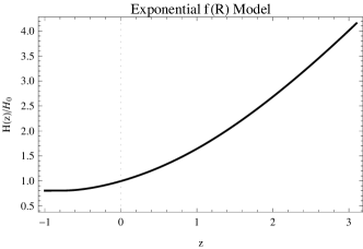
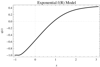
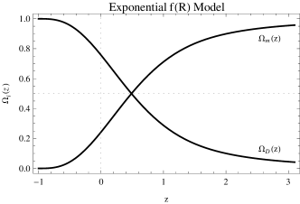
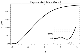
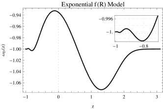
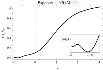
Figure 3: Same as Fig. 1 but for the Exponential model. Auxiliary parameters are $\Omega_{\rm m_{0}}=0.24$, $\Omega_{\rm D_{0}}=0.76$, $\Omega_{\rm rad_{0}}=4.1\times 10^{-5}$ and $\beta=1.8$.

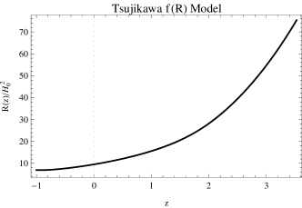
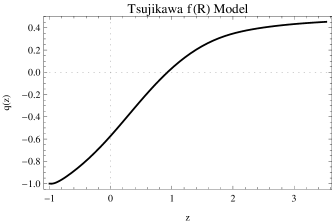
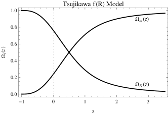
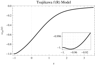
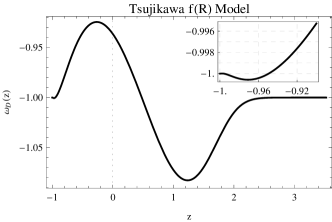
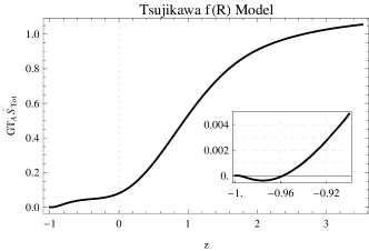
Figure 4: Same as Fig. 1 but for the Tsujikawa model. Auxiliary parameters are $\Omega_{\rm m_{0}}=0.24$, $\Omega_{\rm D_{0}}=0.76$, $\Omega_{\rm rad_{0}}=4.1\times 10^{-5}$ and $\lambda=1$.

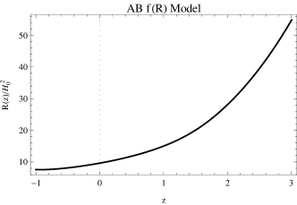
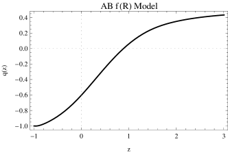
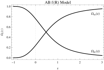
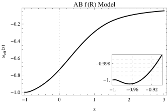
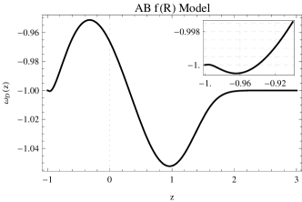
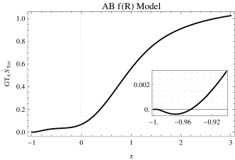
Figure 5: Same as Fig. 1 but for the AB model. Auxiliary parameters are $\Omega_{\rm m_{0}}=0.24$, $\Omega_{\rm D_{0}}=0.76$, $\Omega_{\rm rad_{0}}=4.1\times 10^{-5}$ and $b=1.4$.

With the help of numerical results obtained for $y_{\rm H}(z)$ in Eq. (40), we can obtain the evolutionary behaviors of $H$, $R$, $q$, $\Omega_{\rm m}$, $\Omega_{\rm D}$, $\omega_{\rm eff}$, $\omega_{\rm D}$ and GSL for our selected $f(R)$ models. The results for the Starobinsky, Hu-Sawicki, Exponential, Tsujikawa and AB $f(R)$ models are displayed in Figs. 1-5. Figures show that: (i) the Hubble parameter and the Ricci scalar decrease during history of the universe. (ii) The deceleration parameter $q$ varies from an early matter-dominant epoch ($q=0.5$) to the de Sitter era ($q=-1$) in the future, as expected. It also shows a transition from a cosmic deceleration $q>0$ to the acceleration $q<0$ in the near past. The current values of the deceleration parameter for the Starobinsky, Hu-Sawicki, Exponential, Tsujikawa and AB $f(R)$ models are obtained as $q_{0}=-0.56$, $-0.60$, $-0.56$, $-0.57$ and $-0.60$, respectively. These are in good agreement with the recent observational constraint $q_{0}=-0.43_{-0.17}^{+0.13}~{}(68\%~{}\rm CL)$ obtained by the cosmography CapCosmo . (iii) The density parameters $\Omega_{\rm D}$ and $\Omega_{\rm m}$ increases and decreases, respectively, as $z$ decreases. (iv) The effective EoS parameter, $\omega_{\rm eff}$, for the all models, starts from an early matter-dominated regime (i.e. $\omega_{\rm eff}=0$) and in the late time, $z\rightarrow-1$, it behaves like the $\Lambda$CDM model, $\omega_{\rm eff}\rightarrow-1$. (v) The EoS parameter of DE, $\omega_{\rm D}$, for the all models starts at the phase of a cosmological constant, i.e. $\omega_{\rm D}=-1$, and evolves from the phantom phase, $\omega_{\rm D}<-1$, to the non-phantom (quintessence) phase, $\omega_{\rm D}>-1$. The crossing of the phantom divide line $\omega_{\rm D}=-1$ occurs in the near past as well as farther future. At late times ($z\rightarrow-1$), $\omega_{\rm D}$ approaches again to $-1$ like the $\Lambda$CDM model. Moreover, the present values of $\omega_{\rm D}$ for the Starobinsky, Hu-Sawicki, Exponential, Tsujikawa and AB $f(R)$ models are obtained as $\omega_{\rm D_{0}}=-0.94$, $-0.98$, $-0.93$, $-0.94$ and $-0.97$, respectively. These values satisfy the present observational constraints WMAP ; Planck .

(vi) The variation of the GSL shows that it holds for the aforementioned models from early times to the present epoch. But in the farther future, the GSL for the Starobinsky, Hu-Sawicki, Exponential, Tsujikawa and AB $f(R)$ models is violated for $-0.996<z<-0.955$, $-0.935<z<-0.909$, $-0.897<z<-0.751$, $-0.997<z<-0.958$ and $-0.995<z<-0.950$, respectively. To investigate this problem in ample detail, using Eq. (17) we rewrite Eq. (30) in terms of $\omega_{\rm eff}$ as

$$T_{\rm A}\dot{S}_{\rm tot}=\frac{1}{4G}\left[\frac{9}{2}(1+\omega_{\rm eff})^{2}F+\frac{3}{2}(1+\omega_{\rm eff})\frac{\dot{F}}{H}-(1+3\omega_{\rm eff})\frac{\ddot{F}}{H^{2}}\right],$$ (55)

which shows that in the farther future $z\rightarrow-1$ when $\omega_{\rm eff}\rightarrow-1$ (see Figs. 1-5) we have

$$T_{\rm A}\dot{S}_{\rm tot}\simeq\frac{\ddot{F}}{2GH^{2}}.$$ (56)

According to Eq. (56), the validity of GSL, i.e. $T_{\rm A}\dot{S}_{\rm{tot}}\geq 0$, depends on the sign of $\ddot{F}$. In Figs. 1-5, we plot the variation of $\ddot{F}/(2H^{2})$ versus $z$ in the farther future for the selected $f(R)$ models. Figures confirm that when the sign of $\ddot{F}$ changes from positive to negative due to the dominance of DE over non-relativistic matter then the GSL is violated. Although the parameters used for each model in Figs. 1-5 are the viable ones, by more fine tuning the model parameters the GSL can be held. For instance, in AB $f(R)$ model by choosing the model parameter as $b=1.3$, the GSL is always satisfied from early times to the late cosmological history of the universe.

In Figs. 6-10, we plot the evolutions of $RF_{\rm R}$, $G_{\rm eff}/G$, $g$ and the growth factor $f$ versus $z$ for the selected $f(R)$ models. Figures show that: (i) $RF_{\rm R}$ goes to zero for higher values of $z$ which means that the $f(R)$ models at high $z$ regime behave like the $\Lambda$CDM model. (ii) The screened mass function $G_{\rm eff}/G$ for a given wavenumber $k$ is larger than one which makes a faster growth of the structures compared to the GR. However, for the higher redshifts, the screened mass function approaches to unity in which the GR structure formation is recovered. Note that the deviation of $G_{\rm eff}/G$ from unity for small scale structures (larger $k$) is greater than large scale structures (smaller $k$). (iii) The linear density contrast relative to its value in a pure matter model $g=\delta/a$ starts from an early matter-dominated phase, i.e. $g\simeq 1$ and decreases during history of the universe. For a given $z$, $g$ in the all $f(R)$ models, is greater than that in the $\Lambda$CDM model. (iv) The evolution of the growth factor $f(z)$ for $f(R)$ models and $\Lambda$CDM model together with the 11 observational data of the growth factor listed in Table 1 show that for smaller structures (larger $k$), the all $f(R)$ models deviate from the observational data. But for larger structures (smaller $k$), the growth factor in the all $f(R)$ models, very similar to the $\Lambda$CDM model, fits the data very well.

VIII Conclusions

Here, we investigated the evolution of both matter density fluctuations and GSL in some viable $f(R)$ models containing the Starobinsky, Hu-Sawicki, Exponential, Tsujikawa and AB models. For the aforementioned models, we first obtained the evolutionary behaviors of the Hubble parameter, the Ricci scalar, the deceleration parameter, the matter and DE density parameters, the EoS parameters and the GSL. Then, we explored the growth of structure formation in the selected $f(R)$ models. Our results show the following.

(i) All of the selected $f(R)$ models can give rise to a late time accelerated expansion phase of the universe. The deceleration parameter for the all models shows a cosmic deceleration $q>0$ to acceleration $q<0$ transition. The present value of the deceleration parameter takes place in the observational range. Also at late times ($z\rightarrow-1$), it approaches a de Sitter regime (i.e. $q\rightarrow-1$), as expected.

(ii) The effective EoS parameter $\omega_{\rm eff}$ for the all models starts from the matter dominated era, $\omega_{\rm eff}\simeq 0$, and in the late time, $z\rightarrow-1$, it behaves like the $\Lambda$CDM model, $\omega_{\rm eff}\rightarrow-1$.

(iii) The evolution of the EoS parameter of DE, $\omega_{\rm D}$, shows that the crossing of the phantom divide line $\omega_{D}=-1$ appears in the near past as well as farther future. This is a common physical phenomena to the existing viable $f(R)$ models and thus it is one of the peculiar properties of $f(R)$ gravity models characterizing the deviation from the $\Lambda$CDM model Bamba2 .

(iv) The GSL is respected from the early times to the present epoch. But in the farther future, the GSL for the all models is violated in some ranges of redshift. The physical reason why the GSL does not hold in the farther future is that the sign of $\ddot{F}$ changes from positive to negative due to the dominance of DE over non-relativistic matter.

(v) For the all models, the screened mass function $G_{\rm eff}/G$ is larger than 1 and in high $z$ regime goes to 1. The deviation of $G_{\rm eff}/G$ from unity for larger $k$ (smaller structures) is greater than the smaller $k$ (larger structures). The modification of GR in the framework of $f(R)$-gravity, gives rise to an effective gravitational constant, $G_{\rm eff}$, which is time and scale dependent parameter in contrast to the Newtonian gravitational constant.

(vi) The linear density contrast relative to its value in a pure matter model, $g(a)=\delta_{\rm m}/a$, for the all models starts from an early matter-dominated phase, $g(a)=1$, and decreases during history of the universe.

(vii) The evolutionary behavior of the growth factor of linear matter density perturbations, $f(z)$, shows that for the all models the growth factor for smaller $k$ (larger structures) like the $\Lambda$CDM model fit the data very well.

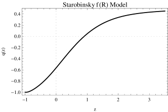
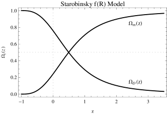
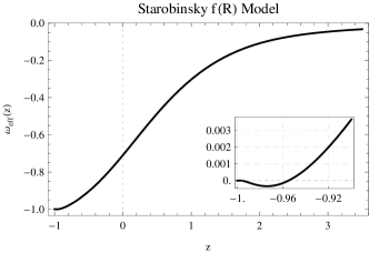
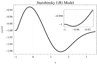
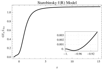
Figure 1: The variations of the Hubble parameter $H/H_{0}$, the Ricci scalar $R/H_{0}^{2}$, the deceleration parameter $q$, the density parameter $\Omega_{\rm i}$, the effective EoS parameter $\omega_{\rm eff}$ , the EoS parameter of DE $\omega_{\rm D}$, the GSL, $GT_{\rm A}\dot{S}_{\rm tot}$ and $\frac{\ddot{F}}{2H^{2}}$ versus redshift $z$ for the Starobinsky model. Auxiliary parameters are $\Omega_{\rm m_{0}}=0.24$, $\Omega_{\rm D_{0}}=0.76$, $\Omega_{\rm rad_{0}}=4.1\times 10^{-5}$, $\lambda=1$ and $n=2$ .

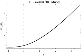
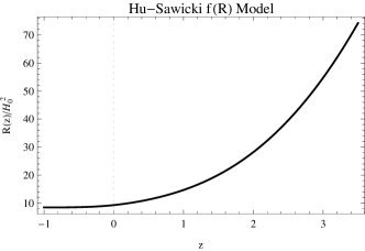
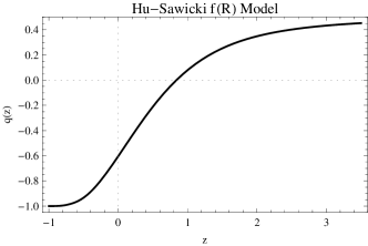
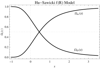
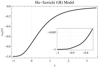
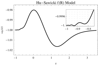
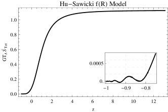
Figure 2: Same as Fig. 1 but for the Hu-Sawicki model. Auxiliary parameters are $\Omega_{\rm m_{0}}=0.24$, $\Omega_{\rm D_{0}}=0.76$, $\Omega_{\rm rad_{0}}=4.1\times 10^{-5}$, $c_{1}=1.25\times 10^{-3}$, $c_{2}=6.56\times 10^{-5}$ and $n=4$.

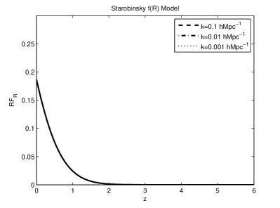
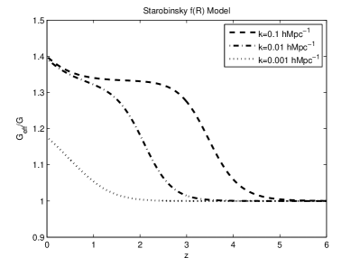
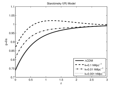
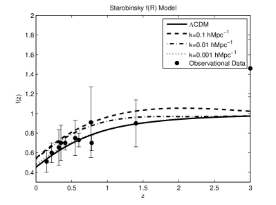
Figure 6: The variations of $RF_{\rm R}$, the screened mass function $G_{\rm eff}/G$, the linear density contrast relative to its value in a pure matter model $g=\delta/a$ and the growth factor $f(z)$, versus redshift $z$ for the Starobinsky model.

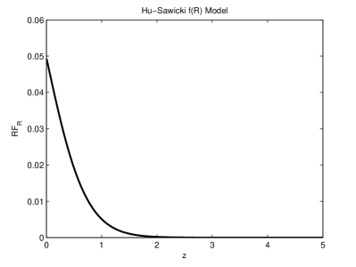
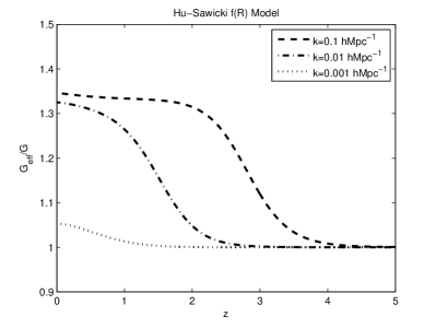
Figure 7: Same as Fig. 6 but for the Hu-Sawicki model.

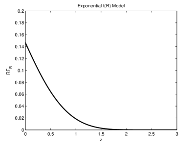
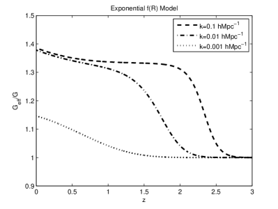
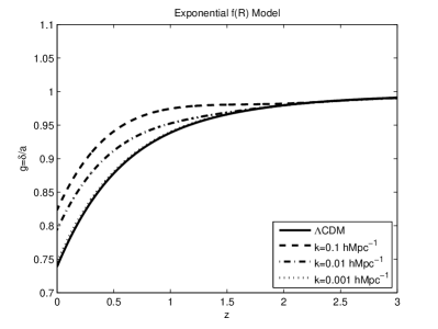
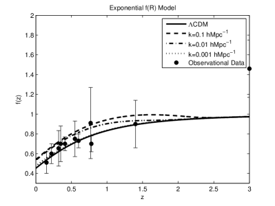
Figure 8: Same as Fig. 6 but for the Exponential model.

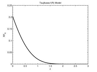
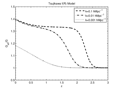
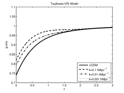
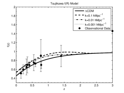
Figure 9: Same as Fig. 6 but for the Tsujikawa model.

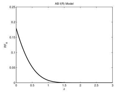
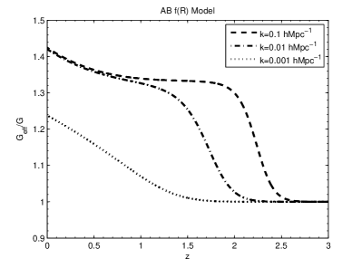
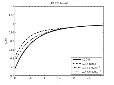
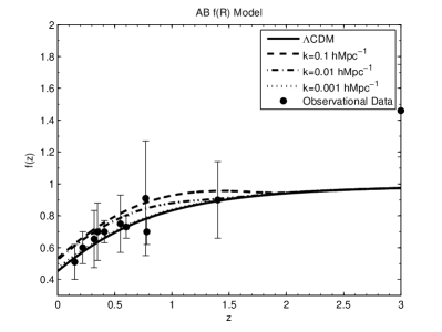
Figure 10: Same as Fig. 6 but for the AB model.

Table 1: The observational data for the linear growth rate $f_{\rm obs}(z)$.

$z$	$0.15$	$0.22$	$0.32$	$0.35$	$0.41$	$0.55$	$0.60$	$0.77$	$0.78$	$1.4$	$3.0$
$f_{\rm obs}$	$0.51$	$0.60$	$0.654$	$0.70$	$0.70$	$0.75$	$0.73$	$0.91$	$0.70$	$0.90$	$1.46$
$1\sigma$	$0.11$	$0.10$	$0.18$	$0.18$	$0.07$	$0.18$	$0.07$	$0.36$	$0.08$	$0.24$	$0.29$
Ref.	Hawkins	Blake	Reyes	Tegmarks	Blake	Ross	Blake	Guzzo	Blake	Angela	Donald

References

- (1) M. Kowalski, et al., (Supernova Cosmology Project), Astrophys. J. 686, 749 (2008).
-
(2)
E. Komatsu, et al., (WMAP Collaboration), Astrophys. J. Suppl. 192, 18 (2011);
G. Hinshaw, et al., (WMAP Collaboration), Astrophys. J. Suppl. 208, 19 (2013). - (3) P.A.R. Ade, et al., (Planck Collaboration), Astron. Astrophys. 571, A16 (2014).
-
(4)
M. Tegmark, et al., (SDSS collaboration), Phys. Rev. D 69,
103501 (2004);
D.J. Eisenstein, et al., (SDSS collaboration), Astrophys. J. 633, 560 (2005);
H. Lampeitl, et al., (SDSS collaboration), Mon. Not. Roy. Astron. Soc. 401, 2331 (2009). -
(5)
T. Padmanabhan, Phys. Rep. 380, 235 (2003);
P.J.E. Peebles, B. Ratra, Rev. Mod. Phys. 75, 559 (2003);
C.G. Tsagas, A. Challinor, R. Maartens, Phys. Rept. 465, 61 (2008);
M. Li, et al., Commun. Theor. Phys. 56, 525 (2011). -
(6)
T.P. Sotiriou, V. Faraoni, Rev. Mod. Phys. 82, 451 (2010);
A. De Felice, S. Tsujikawa, Living Rev. Relativ. 13, 3 (2010);
S. Nojiri, S.D. Odintsov, Phys. Rept. 505, 59 (2011). - (7) S. Nojiri, S.D. Odintsov, Phys. Rev. D 68, 123512 (2003).
- (8) S.A. Appleby, R.A. Battye, A.A. Starobinsky, JCAP 06, 005 (2010).
-
(9)
H. Motohashi, A. Nishizawa, Phys. Rev. D 86, 083514 (2012);
A. Nishizawa, H. Motohashi, Phys. Rev. D 89, 063541 (2014). - (10) Y. Sobouti, Astron. Astrophys. 464, 921 (2007).
-
(11)
K. Karami, M.S. Khaledian, JHEP 03, 086 (2011);
K. Karami, M.S. Khaledian, Int. J. Mod. Phys. D 21, 1250083 (2012). - (12) A. Raccanelli, et al., Mon. Not. Roy. Astron. Soc. 436, 89 (2013).
- (13) D. Huterer, et al., Astropart. Phys. 63, 23 (2015).
- (14) M. Kunz, D. Sapone, Phys. Rev. Lett. 98, 121301 (2007).
- (15) E. Bertschinger, P. Zukin, Phys. Rev. D 78, 024015 (2008).
- (16) S. Baghram, S. Rahvar, JCAP 12, 008 (2010).
- (17) N. Mirzatuny, S. Khosravi, S. Baghram, H. Moshafi, JCAP 01, 019 (2014).
- (18) Y.S. Song, W. Hu, I. Sawicki, Phys. Rev. D 75, 044004 (2007).
- (19) T. Jacobson, Phys. Rev. Lett. 75, 1260 (1995).
- (20) R.G. Cai, S.P. Kim, JHEP 02, 050 (2005).
-
(21)
M. Akbar, R.G. Cai, Phys. Lett. B 635,
7 (2006);
M. Akbar, R.G. Cai, Phys. Lett. B 648, 243 (2007). - (22) K. Karami, M.S. Khaledian, N. Abdollahi, Europhys. Lett. 98, 30010 (2012).
- (23) G. Izquierdo, D. Pavón, Phys. Lett. B 639, 1 (2006).
-
(24)
H. Mohseni Sadjadi, Phys. Rev. D 73, 063525 (2006);
H. Mohseni Sadjadi, Phys. Rev. D 76, 104024 (2007);
H. Mohseni Sadjadi, Phys. Lett. B 645, 108 (2007). - (25) J. Zhou, et al., Phys. Lett. B 652, 86 (2007).
-
(26)
Y. Gong, B. Wang, A. Wang, Phys. Rev. D 75, 123516 (2007);
Y. Gong, B. Wang, A. Wang, JCAP 01, 024 (2007). - (27) M. Jamil, M. Akbar, Gen. Relativ. Gravit. 43, 1061 (2011).
-
(28)
A. Sheykhi, B. Wang, Phys. Lett. B 678, 434 (2009);
A. Sheykhi, Phys. Rev. D 81, 104011 (2010). - (29) N. Banerjee, D. Pavón, Phys. Lett. B 647, 447 (2007).
-
(30)
K. Karami, JCAP 01, 015 (2010);
K. Karami, S. Ghaffari, Phys. Lett. B 685, 115 (2010);
K. Karami, S. Ghaffari, Phys. Lett. B 688, 125 (2010);
K. Karami, S. Ghaffari, M.M. Soltanzadeh, Class. Quantum Grav. 27, 205021 (2010). -
(31)
K. Karami, et al., JHEP 08, 150 (2011);
K. Karami, A. Abdolmaleki, JCAP 04, 007 (2012);
K. Karami, et al., Eur. Phys. J. C 73, 2565 (2013);
K. Karami, et al., Phys. Rev. D 88, 084034 (2013);
A. Abdolmaleki, T. Najafi, K. Karami, Phys. Rev. D 89, 104041 (2014). - (32) N. Radicella, D. Pavón, Phys. Lett. B 691, 121 (2010).
- (33) K. Bamba, C.Q. Geng, JCAP 11, 008 (2011).
- (34) A.A. Starobinsky, Phys. Lett. B 91, 99 (1980).
-
(35)
H. Motohashi, A.A. Starobinsky, J. Yokoyama, Prog. Theor. Phys. 123, 887 (2010);
H. Motohashi, A.A. Starobinsky, J. Yokoyama, JCAP 06, 006 (2011). -
(36)
S. Capozziello, et al., Int. J. Mod. Phys. D 12 1969, (2003);
S. Capozziello, V.F. Cardone, A. Troisi, Phys. Rev. D 71, 043503 (2005). -
(37)
N.J. Poplawski, Phys. Lett. B 640, 135 (2006);
S. Capozzielo, et al., Astrophys. Space Sci. 342, 155 (2012);
V.F. Cardone, S. Camera, A. Diaferio, JCAP 02, 030 (2012). - (38) J.c. Hwang, H. Noh, Phys. Rev. D 71, 063536 (2005).
- (39) S. Tsujikawa, Phys. Rev. D 77, 023507 (2008).
- (40) A.A. Starobinsky, JETP Lett. 86, 157 (2007).
-
(41)
S. Tsujikawa, Phys. Rev. D 76, 023514 (2007);
S. Tsujikawa, K. Uddin, R. Tavakol, Phys. Rev. D 77, 043007 (2008). - (42) H. Motohashi, A.A. Starobinsky, J. Yokoyama, Int. J. Mod. Phys. D 18, 1731 (2009).
-
(43)
P.J.E. Peebles, Principles of Physical Cosmology, Princeton University Press (1993);
T. Padmanabhan, Structure formation in the universe, Cambridge University Press (1993). - (44) J.D. Bekenstein, Phys. Rev. D 9, 3292 (1974).
-
(45)
R.M. Wald, Phys. Rev. D 48, 3427 (1993);
G. Cognola, et al., JCAP 02, 010 (2005). - (46) L.G. Jaime, L. Patiño, M. Salgado, arXiv:1206.1642.
- (47) W. Hu, I. Sawicki, Phys. Rev. D 76, 064004 (2007).
- (48) K. Bamba, C.Q. Geng, C.C. Lee, JCAP 08, 021 (2010).
- (49) A.D. Dolgav, M. Kawasaki, Phys. Lett. B 573, 1 (2003).
- (50) V. Faraoni, Phys. Rev. D 74, 104017 (2006).
- (51) S. Tsujikawa, et al., Phys. Rev. D 80, 084044 (2009).
- (52) A. de la Cruz-Dombriz, A. Dobado, A.L. Maroto, Phys. Rev. Lett. 103, 179001 (2009).
- (53) H. Motohashi, A.A. Starobinsky, J. Yokoyama, Int. J. Mod. Phys. D 20, 1347 (2011).
-
(54)
K. Bamba, C.Q. Geng, C.C. Lee, JCAP 11, 001 (2010);
K. Bamba, C.Q. Geng, C.C. Lee, Int. J. Mod. Phys. D 20, 1339 (2011). -
(55)
S.A. Appleby, R.A. Battye, Phys. Lett. B
654, 7 (2007);
S.A. Appleby, R.A. Battye, JCAP 05, 019 (2008). - (56) S. Capozziello, et al., Phys. Rev. D 84, 043527 (2011).
-
(57)
L. Verde, et al., Mon. Not. Roy. Astron. Soc. 335, 432 (2002);
E. Hawkins, et al., Mon. Not. Roy. Astron. Soc. 346, 78 (2003);
E.V. Linder, Astropart. Phys. 29, 336 (2008). - (58) C. Blake, et al., Mon. Not. Roy. Astron. Soc. 415, 2876 (2011).
- (59) R. Reyes, et al., Nature 464, 256 (2010).
- (60) M. Tegmark, et al., Phys. Rev. D 74, 123507 (2006).
- (61) N.P. Ross, et al., Mon. Not. Roy. Astron. Soc. 381, 573 (2007).
- (62) L. Guzzo, et al., Nature 451, 541 (2008).
- (63) J. da Angela, et al., Mon. Not. Roy. Astron. Soc. 383, 565 (2008).
- (64) P. McDonald, et al., Astrophys. J. 635, 761 (2005).