A highly stable atomic vector magnetometer based on free spin precession

Abstract

We present a magnetometer based on optically pumped Cs atoms that measures the magnitude and direction of a $1\text{\,}\mathrm{\SIUnitSymbolMicro}\mathrm{T}$ magnetic field. Multiple circularly polarized laser beams were used to probe the free spin precession of the Cs atoms. The design was optimized for long-time stability and achieves a scalar resolution better than $300\text{\,}\mathrm{f}\mathrm{T}$ for integration times ranging from $80\text{\,}\mathrm{m}\mathrm{s}$ to $1000\text{\,}\mathrm{s}$. The best scalar resolution of less than $80\text{\,}\mathrm{f}\mathrm{T}$ was reached with integration times of 1.6 to $6\text{\,}\mathrm{s}$. We were able to measure the magnetic field direction with a resolution better than $10\text{\,}\mathrm{\SIUnitSymbolMicro}\mathrm{r}\mathrm{a}\mathrm{d}$ for integration times from $10\text{\,}\mathrm{s}$ up to $2000\text{\,}\mathrm{s}$.

1 Introduction

Magnetometers using optical pumping (OPM) of atomic media were pioneered in the early 1960s [1]. Since then, many OPM varieties [2] have been developed for diverse applications, e.g., mapping the geo-magnetic field or detection of the bio-magnetic field emanating from the human heart [3, 4] and brain [5, 6]. In fundamental science, OPMs monitor the magnetic field in precision magnetic resonance experiments searching for electric dipole moments (EDM) [7, 8] and Lorentz invariance tests [9, 10]. The neutron EDM (nEDM) search sets stringent constraints on theories proposing extensions beyond the standard model of particle physics. Experimental sensitivity to a nEDM depends directly on the control and measurement of the magnetic field in the experiment, a task of particular challenge since (currently) the field must be known over volumes on the order of 20 l for times of hundreds of seconds. Herein, we present an OPM combining long-term stability with high statistical sensitivity, and including vector information. The OPM is designed to serve in an array of such sensors to form an auxiliary magnetometer system monitoring the stability and uniformity of the magnetic field in a next generation nEDM experiment at the Paul Scherrer Institut. An array of scalar Cs OPMs has been used successfully to determine directional and gradient magnetic field information via fits to multi-sensor readings [11].

Various methods exist for extracting information about the magnetic field vector components, including the spin exchange relaxation free (SERF) magnetometers [5] operating at $|{\mathbf{B}}_{0}|=0$ and whose intrinsically sensitivity is to one vector component only. For operation in the offset fields used for neutron magnetic resonance, we focus on conventional OPMs that measure the magnetic field modulus by detecting the Larmor precession frequency, $\omega_{\mathrm{L}}=\gamma|{\mathbf{B}}_{0}|$, where $\gamma$ is the gyromagnetic ratio of the probed atomic state. Information about vector components is gleaned by monitoring the OPM’s response to an externally applied oscillating magnetic field using phase sensitive detection. In a recently published all-optical variant of that method [12], circularly polarized laser beams induce an effect equivalent to the perturbation field via the vector light shift [13]. Without external modulations, vector information can be inferred using multiple detection channels [14] when the first and second harmonics of the Larmor precession of an atomic alignment [15] are detected with linearly polarized light.

Our approach uses multiple circularly polarized laser beams to gain vector information and thus extends methods pioneered by Fairweather and Usher [16]. The absorption of circularly polarized light depends linearly on the projection of the atomic spin polarization on the light’s ${\mathbf{k}}$ vector. The precessing atomic polarization modulates the transmitted light power at $\omega_{L}$ if ${\mathbf{B}}_{0}$ is not parallel to ${\mathbf{k}}$. This can be used to maintain the condition ${\mathbf{B}}_{0}\parallel{\mathbf{k}}$ in a feedback loop either by changing the direction of ${\mathbf{B}}_{0}$ [16] or of ${\mathbf{k}}$ [17]. In contrast to those vector magnetometer implementations, our system uses off-line data analysis enabling us to infer the magnetic field information from free spin precession (FSP) signals. The FSP method is particularly well suited for the application in nEDM experiments since it allows for very stable field measurements.

2 Experimental setup

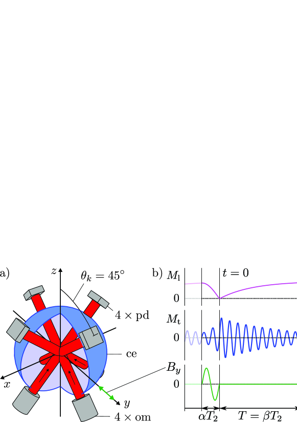
Figure 1: a) Apparatus schematic: four laser light beams are polarized by the optical modules (om), traverse the Cs cell (ce, shown in section) and are converted into signals $S_{i}$ by the photodiodes (pd). b) Measurement cycle time structure, repeated every $40\,\mathrm{ms}$: The longitudinal magnetization $M_{\mathrm{l}}$ is created by optical pumping. Following a $\pi/2$ pulse, $B_{y}$, of duration $\alpha T_{2}$, the resultant transverse magnetization $M_{\mathrm{t}}$ gives rise to FSP signals (shown here projected onto the $x$ axis). The parameters $\alpha,\beta$ measure the length of the $\pi/2$ pulse and the FSP signal, respectively, in units of $T_{2}$. In each signal analysis, the $t=0$ time origin is reset to the FSP start.

The experiment was performed inside the magnetic shield of the nEDM experiment at PSI [18], in which a stable $1\text{\,}\mathrm{\SIUnitSymbolMicro}\mathrm{T}$ magnetic field was generated by a $\cos\theta$ coil. The static magnetic field is parametrized as ${\mathbf{B}}_{0}=B_{0}(\sin\theta\cos\phi,\sin\theta\sin\phi,$ $\cos\theta)$, and was approximately aligned along the $z$ axis, i.e., $\theta\approx 0$. Our magnetometer was created to measure the field modulus, $B_{0}$, and its direction, i.e., the polar angle, $\theta$, and azimuthal angle $\phi$. The magnetometer design is shown in Fig. 1(a). Light is generated by an extended cavity diode-laser coupled to a polarization-maintaining single-mode fiber splitter having three outputs. One output feeds a saturated absorption spectroscopy unit, used for active laser frequency stabilization to the $F{=}4\rightarrow 3$ cesium $D_{1}$ transition ($894\text{\,}\mathrm{n}\mathrm{m}$). A second single-mode fiber guides light to the magnetometer head, where it is split into four beams which are coupled into short multi-mode fibers. At the sensor head, the light from each multi-mode fiber is collimated and circularly polarized by a linear polarizer and a quarter-wave plate, mounted in a compact optical module (om). The power of those beams can be adjusted by rotating an additional linear polarizer in the om. The beams traverse an evacuated $45\text{\,}\mathrm{m}\mathrm{m}$ diameter glass-cell (ce) containing a saturated vapor of cesium atoms. The cell is paraffin coated [19] to reduce spin depolarization during atom-wall collisions. A combination of photodiodes (pd) and transimpedance amplifiers converts the transmitted light power of each beam to a signal $S_{i}$, which is digitized with a high resolution sampling system. The combined noise of the photodiode, preamp, and sampling system is well below the shot-noise level for the typical light power of $1\text{\,}\mathrm{\SIUnitSymbolMicro}\mathrm{W}$ per laser beam.

The magnetometer is operated in pulsed mode, and information is extracted from the FSP signals. Figure 1(b) shows the experimental cycle which repeats every 40 ms. The FSP is described using the magnetization ${\mathbf{M}}$ associated with the ensemble average of the atomic spin. The combined optical pumping by the four laser beams in combination with ${\mathbf{B}}_{0}$ creates a magnetization ${\mathbf{M}}_{\mathrm{l}}$ longitudinal to ${\mathbf{B}}_{0}$. A short magnetic $\pi/2$ pulse along the $y$ direction turns ${\mathbf{M}}_{\mathrm{l}}$ to a direction transverse to ${\mathbf{B}}_{0}$, creating ${\mathbf{M}}_{\mathrm{t}}$. The pulse uses a single sinusoidal period in order to minimize deadtime ($\alpha$ in Fig. 1(b)). The magnetization component perpendicular to ${\mathbf{B}}_{0}$ precesses at the Larmor frequency, $\omega_{\mathrm{L}}=\gamma B_{0}$, where $\gamma=$3.498\,621\,1(4)\text{\,}\mathrm{k}\mathrm{H}\mathrm{z}\mathrm{/}\mathrm{\SIUnitSymbolMicro}\mathrm{T}$$ is the gyromagnetic ratio of the $F{=}4$ cesium ground state. The light absorption by the cesium atoms depends linearly on the projection of ${\mathbf{M}}$ on the light’s $k$-vector [20]. Consequently, the transmitted laser power, measured by a photodiode, is modulated at $\omega_{\mathrm{L}}$. The transverse magnetization component decay (see $M_{\mathrm{t}}$ in Fig. 1(b)), with its effective decay time $T_{2}$, is observed as a decreasing modulation amplitude of the recorded FSP photodiode signal. During the FSP, the longitudinal magnetization, $M_{\mathrm{l}}$, is recreated by optical pumping, such that the next $\pi/2$ pulse can start the next cycle. Both the data acquisition system recording the FSP signals and the function generator producing the $\pi/2$ pulses are synchronized to an atomic clock.

Using the classical Bloch equation, the recorded signal for each laser beam can be modeled as

$$S_{i}(t)=c_{i}+e^{-\frac{t}{T_{2}}}\left(b_{i}+A_{\mathrm{c},i}\cos{\omega t}+A_{\mathrm{s},i}\sin{\omega t}\right)\,.$$ (1)

Both frequency $\omega$ and effective decay time $T_{2}$ are common parameters for all simultaneously recorded FSP signals. The offsets, $c_{i}$ and $b_{i}$, as well as the in-phase, $A_{\mathrm{c},i}$, and quadrature, $A_{\mathrm{s},i}$, components of the modulation amplitudes are different for each signal $S_{i}$. The $c_{i}$ parameters represent the DC signal offsets and are proportional to the average light power of beam $i$. If the $k$-vector of beam $i$ has a longitudinal component, the exponential build-up of $M_{\mathrm{l}}$ contributes to the absorption it probes. Assuming that the longitudinal and transverse relaxation rates are equal allows this contribution to be parametrized by the offsets $b_{i}$. The modulation amplitudes are used to determine the magnetic field direction. The ${\mathbf{B}}_{0}$ field magnitude is determined using the estimation of frequency $\omega$, interpreted as the Larmor frequency. The magnitude and the extracted field direction are used to reconstruct the vector magnetic field.

3 Data analysis

The parameters of Eq. (1) are extracted with a precision limited by the Cramér-Rao Lower Bound (CRLB) [21, 22]. The lower limit of the frequency spectral density, $\rho_{f}$, calculated with the CRLB for signals with no DC components ($c_{i}=b_{i}=0$) and sampled at a sufficiently high rate ($\gg\omega_{L}/2\pi$) is

$$\rho_{f}\geq\frac{2\,\rho}{\pi\,A\,T_{2}}\sqrt{\frac{\left(\alpha+\beta\right)e^{\beta}\sinh\beta}{\cosh 2\beta-2\beta^{2}-1}}\,.$$ (2)

The length of the FSP signal, $T$, is parametrized in a dimensionless way by $\beta=T/T_{2}$ (Fig. 1(b)), whereas $\alpha$ measures the dead-time of the $\pi/2$ pulse. The spectral density $\rho$ of the photodiode signals is ultimately limited by shot noise. The amplitude $A$ is proportional to $M_{z}$, in the instance before it is flipped, it thus scales like $A=A_{0}\left(1-e^{-\beta}\right)$. Given this, Eq. (2) has a minimum at $\beta\approx 2.6$. For technical reasons, the pulse repetition time of $T=40\,\mathrm{ms}$ was chosen to be slightly shorter than the optimum given that $T_{2}=20.4(2)~{}\mathrm{ms}$. Estimates indicate a $\sim 10\%$ performance gain at $T\approx 2.6~{}T_{2}$.

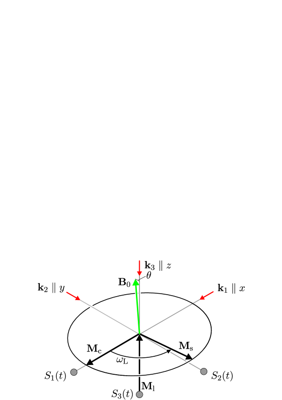
Figure 2: The Larmor precession is described by ${\mathbf{M}}_{\mathrm{c}}$ and ${\mathbf{M}}_{\mathrm{s}}$, c.f. Eq. (3), which together define a plane perpendicular to ${\mathbf{B}}_{0}$ (here depicted as a circle. The longitudinal magnetization ${\mathbf{M}}_{\mathrm{l}}$ changes only slowly due to relaxation and optical pumping. Signal $S_{i}(t)$ represents the transmitted power of the laser beam ${\mathbf{k}}_{i}$.

Reconstructing the ${\mathbf{B}}_{0}$ vector components is made by monitoring the ${\mathbf{M}}$ component precessing at $\omega_{L}$. By definition, the precession happens in a plane perpendicular to ${\mathbf{B}}_{0}$, thus the cross product of two vectors in that plane yields a vector parallel to ${\mathbf{B}}_{0}$. The method’s statistical sensitivity is maximized when the phase difference of the two vectors is $\pi/2$. This is achieved by parametrizing the precessing part of ${\mathbf{M}}$ by its in-phase and quadrature components as

$${\mathbf{M}}_{\mathrm{t}}(t)={\mathbf{M}}_{\mathrm{c}}\cos\omega_{\mathrm{L}}t+{\mathbf{M}}_{\mathrm{s}}\sin\omega_{\mathrm{L}}t\,.$$ (3)

If the two vectors are known, the ${\mathbf{B}}_{0}$ direction follows as

$${\mathbf{B}}_{0}\propto{\mathbf{M}}_{\mathrm{c}}\times{\mathbf{M}}_{\mathrm{s}}.$$ (4)

Measuring ${\mathbf{M}}_{\mathrm{c}}$ and ${\mathbf{M}}_{\mathrm{s}}$ is straightforward in a three-beam magnetometer with orientations along the Cartesian coordinates axes (Fig. 2). In such a configuration, the $\cos$ and $\sin$ modulation components seen by each beam (Eq. (1)) correspond directly to ${\mathbf{M}}_{\mathrm{c}}$ and ${\mathbf{M}}_{\mathrm{s}}$.

The experimental vector magnetometer reported herein uses four laser beams (Fig. 1(a)). In this configuration, each beam has a ${\mathbf{k}}$ component along $z$, thus contributing to optical pumping provided ${\mathbf{B}}_{0}$ is approximately oriented along $z$, which is our case. Each beam probes the projection, $M_{i}=\hat{k}_{i}\cdot{\mathbf{M}}$, of the magnetization ${\mathbf{M}}$ onto its $k$-vector. The 3D vector ${\mathbf{M}}$ is reconstructed from the four projections, using the projection matrix $P$

$$\left(\begin{matrix}M_{x}\\ M_{y}\\ M_{z}\end{matrix}\right)=P\cdot\left(\begin{matrix}M_{1}\\ M_{2}\\ M_{3}\\ M_{4}\end{matrix}\right)\text{\!, \,}P=\frac{1}{\sqrt{2}}\left(\begin{matrix}-1&1&0&0\\ 0&0&-1&1\\ \frac{1}{2}&\frac{1}{2}&\frac{1}{2}&\frac{1}{2}\end{matrix}\right)\,.$$ (5)

This reconstruction is advantageous since $M_{x}$ and $M_{y}$ are derived by subtracting two projections, reducing common mode noise. Since $M_{x}$ and $M_{y}$ are the important components for determining the Larmor frequency, the chosen beam configuration facilitates its high resolution extraction. All parts of the signal $S_{i}(t)$ (Eq. (1)) that depend linearly on ${\mathbf{M}}$ are transformed from the four projections into a 3D representation using the matrix $P$. In the low light-power limit, the in-phase and quadrature modulation amplitudes of $S_{i}(t)$ are proportional to the DC signal, $c_{i}$, detected by photodiode $i$. Amplitudes $A_{\mathrm{c},i}$ and $A_{\mathrm{s},i}$ are normalized using $c_{i}$, to compensate for slight differences in light power and possible differences in photodiode preamplification factors. Finally, $P$ converts the normalized amplitudes extracted from signals $S_{i}(t)$ to 3D vectors that determine the direction of ${\mathbf{B}}_{0}$ using Eq. (4). Using numerical simulations [23], we verified that the resulting angles $\theta$ and $\phi$ are determined with maximum statistical efficiency. The magnetic field direction and magnitude can be extracted from the data of only three laser beams. Given the geometry of the beams in the experiment this is, however, not possible at maximum statistical efficiency. Correlations in the signals $S_{i}(t)$ due to the over determined measurement with four laser beams can be used to verify the normalization factors of the amplitudes [23].

The projection matrix $P$ depends on the actual orientation of the laser beams. Deviations from the assumed orientations lead to systematic errors in the extracted magnetic field orientation $\theta$ and $\phi$. Those errors depend in a complex way on the orientation of the magnetic field and the direction in which the beam is tilted. If one laser beam is tilted by an angle $\Delta\alpha$ in a direction that causes the largest errors, it contributes an error of $\Delta\theta=1/4\,\Delta\alpha$ to the extracted magnetic field orientation. Tilting all four laser beams in this way is equivalent to tilting the whole sensor by $\Delta\alpha$ which naturally causes an estimation error of $\Delta\theta=\Delta\alpha$. Tilting all beams in random directions causes a combined error of $\Delta\theta=1/2\,\Delta\alpha$. The mechanical construction of the experiment can currently not guarantee a alignment better than $\Delta\alpha=0.004$ rad.

Two estimation methods to extract the parameters of Eq. (1) from the digitized signals were studied: Least-squares fitting, and demodulation. The least-squares method fits the Eq. (1) model to the experimental data gained from all beams simultaneously.

The demodulation method uses two-phase lock-in detection with $\cos$ and $\sin$ reference signals at a frequency $\omega_{\mathrm{r}}$ close to $\omega_{\mathrm{L}}$. This mixes the $\omega_{\mathrm{L}}$ modulation down to a frequency close to DC, while noise and other modulations are suppressed by the low-pass filter [24]. The in-phase and quadrature lock-in signals are converted to phase $\varphi(t_{j})\equiv\varphi_{j}$ and amplitude $A(t_{j})\equiv A_{j}$ for each FSP signal. The initial modulation amplitude, $A(t=0)$, is extracted by a least-squares fit of $A(0)\exp{-t/T_{2}}$ to the time series $A_{j}$ of one FSP. The model $\varphi(t)=\varphi(0)+\omega t$ is fitted (with weighting factors $1/A^{2}_{j}$) to the phase signal after correcting for discrete $2\pi$ steps. The frequency difference between $\omega_{\mathrm{r}}$ and $\omega_{\mathrm{L}}$ is found using the slope $\omega$.

The in-phase and quadrature modulation amplitudes are found via $A_{\mathrm{c},i}=A\cos{\varphi(0)}$, and $A_{\mathrm{s},i}=-A\sin{\varphi(0)}$. For both methods, the least-squares fits are made simultaneously for the four FSP signals using one common frequency, $\omega$, and decay time, $T_{2}$.

4 Results

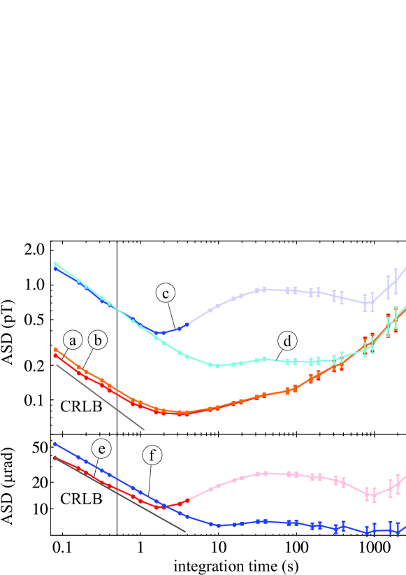
Figure 3: ASD of the magnetic field magnitude (a, b), the field’s z-component (c, d), and the $B$ direction $\theta$ (e, f) measured with the vector cesium magnetometer. The results obtained by least-squares fitting (curves a, c, and e) generally show better ASD values at short integration times, while the demodulation method (curves b, d, f) provides better results over longer integration times. Curves c and e are affected by systematic errors for integration times larger than 4 s. The error bars were calculated according to [25].

The nEDM experiment requires magnetic field measurements that are stable over hundreds of seconds at the sub-pT level. The cesium vector magnetometer statistical errors, as described by the CRLB, are by far sufficient to reach that goal. However, systematic errors arising from drifting parameters limit the long-term stability that this magnetometer can achieve. To characterize the long-term stability, we measured during 11 hours under best-case conditions of field stability. Figure 3 shows the Allan standard deviation (ASD) [26] of vector and scalar field measurements as a function of integration time $\tau$. Using the estimated FSP parameters and a noise density extracted from the measured data’s Fourier spectrum, Eq. (2) yields a CRLB of for the field magnitude. For $\tau<$1\text{\,}\mathrm{s}$$, the ASD plots show the expected improvement proportional to $\tau^{-1/2}$. The least-squares fitting possesses a higher statistical efficiency, which is visible as a $12\%$ smaller ASD. This difference disappears for $\tau>$1\text{\,}\mathrm{s}$$ where the ASD is no longer limited by statistical processes. For the longer integration times, the ASD is limited by magnetic field drifts and magnetometer instabilities, thus, the ASD represents the limit for the magnetometer stability. The magnitude can be measured with an uncertainty smaller than $300\text{\,}\mathrm{f}\mathrm{T}$ for integration times ranging from $80\text{\,}\mathrm{m}\mathrm{s}$ to $1000\text{\,}\mathrm{s}$. A best sensitivity of $75.2\text{\,}\mathrm{f}\mathrm{T}$ is achieved at $\tau=$4\text{\,}\mathrm{s}$$, which corresponds to a relative sensitivity of $7.6\times 10^{-8}$.

Curves c and d in Fig. 3 show the ASD for the field’s $z$ component (longitudinal) measurement. This shows that the values extracted using the demodulation method are more stable than those from least-squares fitting for long integration times. This happens because the least-squares fitting does not model the second harmonic of the Larmor modulation, $2\omega_{\mathrm{L}}$, while the demodulation method is insensitive to it due to the low-pass filter. The integration times for which the $z$ component can be measured with an uncertainty smaller than $300\text{\,}\mathrm{f}\mathrm{T}$ range up to $1000\text{\,}\mathrm{s}$, but start at $2\text{\,}\mathrm{s}$, due to the larger statistical errors. This increase in statistical uncertainty is due to using amplitudes which cannot be estimated as precisely as the Larmor frequency.

Figure 3 e and f show the ASD of $\theta$, characterizing the direction ${\mathbf{B}}_{0}$, as derived from the estimated vector components. The ASD of $\theta$, estimated using least-squares fitting, scales statistically for $\tau<$1\text{\,}\mathrm{s}$$ and complies very well with the CRLB calculated using error propagation from the estimated amplitudes. Using demodulation, the resolution of $\theta$ reaches $6.4\text{\,}\mathrm{\SIUnitSymbolMicro}\mathrm{r}\mathrm{a}\mathrm{d}$ for $\tau=$10\text{\,}\mathrm{s}$$, and does not change significantly until $\tau=$2000\text{\,}\mathrm{s}$$. The ASD of $\phi$ behaves similarly, but with larger uncertainties since the measurement was made near the degenerate case of $\theta{=}0$.

5 Conclusion and discussion

The presented magnetometer achieves high sensitivity both in magnitude and field direction. Upper limits on processes that limit the stability of the magnetometer readings are derived from the ASD plots and show high sensitivity is maintained even at integration times of $1000\text{\,}\mathrm{s}$. This value is probably limited by drifts of the $B_{0}$ field components in the present nEDM experiment. Further studies will try to distinguish between instabilities intrinsic to the magnetometer and external field drifts by using several magnetometer modules.

In contrast to other recently published vector magnetometers [12] the presented approach does not degrade the scalar resolution when extracting vector information. Consequently, it achieves an order of magnitude better scalar resolution while being able to resolve the $B_{0}$ direction with $\delta\theta<$10\text{\,}\mathrm{\SIUnitSymbolMicro}\mathrm{r}\mathrm{a}\mathrm{d}$$ for integration times ranging beyond $2000\text{\,}\mathrm{s}$. This makes the presented approach an ideal choice for applications that use long integration times. For our future nEDM apparatus it is planned to use an array of vector Cs magnetometers in order to monitor the $B_{0}$ field and its gradients. Scaling to multiple sensors is aided by the low needs on laser power and the efficient data processing possible in the demodulation mode.

The magnetometer presented here requires calibration in order to provide absolute field direction information. However, the accuracy of its absolute field magnitude information may be limited—as discussed by Grujic et al in [27]—at the several 10 pT level since $\vec{k}\not\perp\vec{B}_{0}$. The demonstrated stability at long integration times is a necessary step for the future development of such calibration procedures. With the stability proven, the detailed studies of device construction systematics (e.g., perturbations to the values in $P$ (Eq. (5)) and device alignment to an external coordinate system will permit calibration of the device, thus moving it from being a field stability measurement system to a true field measurement system.

A remaining disadvantage of this approach is the non-‘magnetically silent’ $\pi/2$ spin manipulation pulse, which can perturb the environment under study. A straightforward way to overcome this is the use of Bell-Bloom pumping, currently under development within our collaboration [27]. A combination of these two methods is being pursued to provide a sensitive and magnetically silent vector magnetometer for our future nEDM search.

References

- [1] A. L. Bloom, “Principles of operation of the rubidium vapor magnetometer,” Appl. Opt. 1, 61 (1962).
- [2] D. Budker and M. Romalis, “Optical magnetometry,” Nat. Phys. 3, 227–234 (2007).
- [3] G. Bison, R. Wynands, and A. Weis, “A laser-pumped magnetometer for the mapping of human cardiomagnetic fields,” Appl. Phys. B-Lasers O. 76, 325–328 (2003).
- [4] R. Wyllie, M. Kauer, R. Wakai, and T. Walker, “Optical magnetometer array for fetal magnetocardiography,” Opt. Lett. 37, 2247–2249 (2012).
- [5] H. Xia, A. Ben-Amar Baranga, D. Hoffman, and M. V. Romalis, “Magnetoencephalography with an atomic magnetometer,” Appl. Phys. Lett. 89, 211104 (2006).
- [6] T. H. Sander, J. Preusser, R. Mhaskar, J. Kitching, L. Trahms, and S. Knappe, “Magnetoencephalography with a chip-scale atomic magnetometer,” Biomed. Opt. Express 3, 981–990 (2012).
- [7] I. Altarev, Y. Borisov, N. Borovikova, A. Egorov, S. Ivanov, E. Kolomensky, M. Lasakov, V. Nazarenko, A. Pirozhkov, A. Serebrov, Y. Sobolev, E. Shulgina, V. Lobashev, “Search for the neutron electric dipole moment,” Phys. Atom. Nucl. 59, 1152–1170 (1996).
- [8] P. Knowles, G. Bison, N. Castagna, A. Hofer, A. Mtchedlishvili, A. Pazgalev, and A. Weis, “Laser-driven cs magnetometer arrays for magnetic field measurement and control,” Nucl. Instrum. Meth A 611, 306–309 (2009).
- [9] M. Smiciklas, J. M. Brown, L. W. Cheuk, S. J. Smullin, and M. V. Romalis, “New test of local lorentz invariance using a comagnetometer,” Phys. Rev. Lett. 107, 171604 (2011).
- [10] S. K. Peck, D. K. Kim, D. Stein, D. Orbaker, A. Foss, M. T. Hummon, and L. R. Hunter, “Limits on local Lorentz invariance in mercury and cesium,” Phys. Rev. A 86, 012109 (2012).
- [11] S. Afach, C. Baker, G. Ban, G. Bison, K. Bodek, M. Burghoff, Z. Chowdhuri, M. Daum, M. Fertl, B. Franke, P. Geltenbort, K. Green, M. van der Grinten, Z. Grujic, P. Harris, W. Heil, V. Hélaine, R. Henneck, M. Horras, P. Iaydjiev, S. Ivanov, M. Kasprzak, Y. Kermadic, K. Kirch, A. Knecht, H.-C. Koch, J. Krempel, M. Kuzniak, B. Lauss, T. Lefort, Y. Lemière, A. Mtchedlishvili, O. Naviliat-Cuncic, J. Pendlebury, M. Perkowski, E. Pierre, F. Piegsa, G. Pignol, P. Prashanth, G. Quéméner, D. Rebreyend, D. Ries, S. Roccia, P. Schmidt-Wellenburg, A. Schnabel, N. Severijns, D. Shiers, K. Smith, J. Voigt, A. Weis, G. Wyszynski, J. Zejma, J. Zenner, and G. Zsigmond, “A measurement of the neutron to 199Hg magnetic moment ratio,” Phys. Lett. B 739, 128–132 (2014).
- [12] B. Patton, E. Zhivun, D. C. Hovde, and D. Budker, “All-optical vector atomic magnetometer,” Phys. Rev. Lett. 113, 013001 (2014).
- [13] B. S. Mathur, H. Tang, and W. Happer, “Light shifts in the alkali atoms,” Phys. Rev. 171, 11–19 (1968).
- [14] L. Lenci, A. Auyuanet, S. Barreiro, P. Valente, A. Lezama, and H. Failache, “Vectorial atomic magnetometer based on coherent transients of laser absorption in rb vapor,” Phys. Rev. A 89, 043836 (2014).
- [15] A. Weis, G. Bison, and A. S. Pazgalev, “Theory of double resonance magnetometers based on atomic alignment,” Phys. Rev. A 74, 033401 (2006).
- [16] A. J. Fairweather and M. J. Usher, “A vector rubidium magnetometer,” J. Phys. E. Sci. Instrum. 5, 986 (1972).
- [17] A. Vershovskii, “Project of laser-pumped quantum mx magnetometer,” Tech. Phys. Lett. 37, 140–143 (2011).
- [18] C. Baker, G. Ban, K. Bodek, M. Burghoff, Z. Chowdhuri, M. Daum, M. Fertl, B. Franke, P. Geltenbort, K. Green, M. van der Grinten, E. Gutsmiedl, P. Harris, R. Henneck, P. Iaydjiev, S. Ivanov, N. Khomutov, M. Kasprzak, K. Kirch, S. Kistryn, S. Knappe-Gruneberg, A. Knecht, P. Knowles, A. Kozela, B. Lauss, T. Lefort, Y. Lemiere, O. Naviliat-Cuncic, J. Pendlebury, E. Pierre, F. Piegsa, G. Pignol, G. Quemener, S. Roccia, P. Schmidt-Wellenburg, D. Shiers, K. Smith, A. Schnabel, L. Trahms, A. Weis, J. Zejma, J. Zenner, and G. Zsigmond, “The search for the neutron electric dipole moment at the paul scherrer institute,” Phys. Proc. 17, 159–167 (2011).
- [19] N. Castagna, G. Bison, G. Di Domenico, A. Hofer, P. Knowles, C. Macchione, H. Saudan, and A. Weis, “A large sample study of spin relaxation and magnetometric sensitivity of paraffin-coated cs vapor cells,” Appl. Phys. B 96, 763–772 (2009).
- [20] H. G. Dehmelt, “Modulation of a light beam by precessing absorbing atoms,” Phys. Rev. 105, 1924–1925 (1957).
- [21] D. Rife and R. Boorstyn, “Single tone parameter estimation from discrete-time observations,” IEEE T. Inform. Theory 20, 591–598 (1974).
- [22] C. Gemmel, W. Heil, S. Karpuk, K. Lenz, C. Ludwig, Y. Sobolev, K. Tullney, M. Burghoff, W. Kilian, S. Knappe-Grüneberg, W. Müller, A. Schnabel, F. Seifert, L. Trahms, and S. Baeßler, “Ultra-sensitive magnetometry based on free precession of nuclear spins,” Eur. Phys. J. D 57, 303–320 (2010).
- [23] S. Afach, “Development of a cesium vector magnetometer for the neutron EDM experiment,” Ph.D. thesis, ETH-Zürich (2014).
- [24] J. Gaspar, S. F. Chen, A. Gordillo, M. Hepp, P. Ferreyra, and C. Marqués, “Digital lock in amplifier: study, design and development with a digital signal processor,” Microprocess. Microsy. 28, 157 – 162 (2004).
- [25] P. Lesage and C. Audoin, “Characterization of frequency stability: Uncertainty due to the finite number of measurements” IEEE T. Instrum. Meas. 22, 157–161 (1973).
- [26] S. Groeger, G. Bison, P. Knowles, and A. Weis, “A sound card based multi-channel frequency measurement system,” Eur. Phys. J.-Appl. Phys. 33, 221–224 (2006).
- [27] Z. Grujić, P. Koss, G. Bison, and A.Weis, “A sensitive and accurate atomic magnetometer based on free spin precession,” Eur. Phys. J. D 69, 135 (2015).