Defensive Resource Allocation in Social Networks

Abstract

In this work, we are interested on the analysis of competing marketing campaigns between an incumbent who dominates the market and a challenger who wants to enter the market. We are interested in (a) the simultaneous decision of how many resources to allocate to their potential customers to advertise their products for both marketing campaigns, and (b) the optimal allocation on the situation in which the incumbent knows the entrance of the challenger and thus can predict its response. Applying results from game theory, we characterize these optimal strategic resource allocations for the voter model of social networks.

1 Introduction

In contrast to mass marketing, which promotes a product indiscriminately to all potential customers, direct marketing promotes a product only to customers likely to be profitable. Focusing on the latter, Domingos and Richardson [1, 2] incorporated the influence of peers on the decision making process of potential customers deciding between different products or services promoted by competing marketing campaigns. This aggregated value of a customer has been called the network value of a customer.

If we consider that each customer makes a buying decision independently of every other customer, we should only consider his intrinsic value (i.e., the expected profit from sales to him). However, if we consider the often strong influence of her friends, acquaintances, etc., then we should incorporate this peer influence to his value for the marketing campaigns.

In the present work, our focus is different from previous works where their interest is to which potential customers to market, while in our work is on how many resources to allocate to market to potential customers. Moreover, we are interested on the scenario when two competing marketing campaigns need to decide how many resources to allocate to potential customers to advertise their products either simultaneously or where the incumbent can foresee the arrival of the challenger and commit to a strategy. The process and dynamics by which influence is spread is given by the voter model.

1.1 Related Works

The (meta) problem of influence maximization was first defined by Domingos and Richardson [1, 2], where they studied a probabilistic setting of this problem and provided heuristics to compute a spread maximizing set. Based on the results of Nemhauser et al. [3], Kempe et al. [4, 5] and Mossel and Roch [6] proved that for very natural activation functions, the function of the expected number of active nodes at termination is a submodular function and thus can be approximated through a greedy approach with a $(1-1/e-\varepsilon)$-approximation algorithm for the spread maximization set problem. A slightly different model but with similar flavor, the voter model, was introduced by Clifford and Sudbury [7] and Holley and Liggett [8]. In that model of social network, Even-Dar and Shapira [9] found an exact solution to the spread maximization set problem when all the nodes have the same cost.

Competitive influence in social networks has been studied in other scenarios. Bharathi et al. [10] proposed a generalization of the independent cascade model [11] and gave a $(1-1/e)$ approximation algorithm for computing the best response to an already known opponent’s strategy. Sanjeev and Kearns [12] studied the case of two players simultaneously choosing some nodes to initially seed while considering two independent functions for the consumers denoted switching function and selection function. Borodin et al. [13] showed that for a broad family of competitive influence models it is NP-hard to achieve an approximation that is better than the square root of the optimal solution. Chasparis and Shamma [14] found optimal advertising policies using dynamic programming on some particular models of social networks.

Within the general context of competitive contests, there is an extensive literature (see e.g. [15, 16, 17, 18]), however their focus is mainly on the case when the contest success function is given by the marketing campaign that put the maximum resources. In that case, Powell [19] studied the sequential, non-zero sum game who has a pure strategy subgame perfect equilibrium where the defender always plays the same pure strategy in any equilibrium, and the attacker’s equilibrium response is generically unique and entails no mixing. Friedman [20] studied the Nash equilibrium when the valuations for both marketing campaigns are the same.

2 Model

Consider two firms: an incumbent (or defender) $D$ and a challenger (or attacker) $A$. Consider the set $\mathcal{N}=\{1,2,\ldots,n\}$ of potential customers. The challenger decides to launch a viral marketing campaign at time $t_{0}=0$ (we will also refer to the viral marketing campaign as an attack). The budget for the challenger is given by $B_{A}\geq 0$. The incumbent $D$ decides to allocate a budget $B_{D}\geq 0$ at time $t_{0}$ to prevent its customers to switch. The players of the game are the competing marketing campaigns and the nodes correspond to the potential customers.

The strategy for player $i$, where $i\in\{D,A\}$, consists on an allocation vector ${\bf x}_{i}=(x_{i,1},x_{i,2}\ldots,x_{i,n})$ where $x_{i,j}$ represents the budget allocated by player $i$ to customer $j$ (e.g., through promotions or offers). Therefore, the set of strategies is given by the $(n-1)$-dimensional simplex

$$\Delta_{i}=\{ (x_{i,1},\ldots,x_{i,n}):$$

$$x_{i,j}\geq 0,\forall\,1\leq j\leq n\quad\textrm{and}\quad\sum_{j=1}^{n}x_{i,j}=B_{i}\}.$$

We consider each potential customer as a component contest. Let $p_{i,j}(x_{i,j},x_{-i,j})$, henceforth the contest success function (CSF), denote the probability that player $i$ wins component contest $j$ when player $i$ allocates $x_{i,j}$ resources and the adversary player $-i$ allocates $x_{-i,j}$ resources to component contest $j$. We assume that the CSF for a player $i$ is proportional to the share of total advertising expenditure on customer $j$, i.e.,

$$p_{i,j}(x_{i,j},x_{-i,j})=\left\{\begin{array}[]{cl}\frac{x_{i,j}}{x_{i,j}+x_{-i,j}}&\textrm{if }x_{i,j}\neq 0\textrm{ or }x_{i,j}\neq 0,\\ \frac{1}{2}&\textrm{if }x_{i,j}=x_{-i,j}=0.\end{array}\right.$$ (1)

Both firms may have different valuations for different customers. The intrinsic value for player $i$ of customer $j$ is given by $w_{i,j}$ where $i\in\{D,A\}$ and $1\leq j\leq N$. The intrinsic payoff function for player $i$ is given by

$$\pi({\bf x}_{i},{\bf x}_{-i},{\bf w}_{i})=\sum_{j=1}^{n}w_{i,j}p_{i,j}(x_{i,j},x_{-i,j}),$$ (2)

where ${\bf w}_{i}=(w_{i,1},w_{i,2},\ldots,w_{i,n})$.

We are interested as well on the network value of a customer. In the next subsection we will compute this.

2.1 Network value of a customer

Let $G=(V,E)$ be an undirected graph with self-loops where $V$ is the set of nodes in the graph which represent the potential customers of the competing marketing campaigns and $E$ is the set of edges which represent the influence between individuals. We denote by $\lvert S\rvert$ the cardinality of the set $S$, by the index $i$ to one of the two players ($D$ or $A$) and by the index $-i$ to the opponent of player $i$. We consider that the graph $G$ has $n$ nodes, i.e. $\lvert V\rvert=n$. For a node $j\in V$, we denote by $N(j)$ the set of neighbors of $j$ in $G$, i.e. $N(j)=\{j^{\prime}\in V:\{j,j^{\prime}\}\in E\}$ and by $d_{j}$ the degree of node $j$, i.e. $d_{j}=\lvert N(j)\rvert$.

We consider two labeling functions for a node $j\in V$ given by its initial preference between different players, $D$ or $A$, denoted by functions $f_{A}^{0}$ and $f_{D}^{0}$ respectively. We denote by $f^{0}_{i}(v)=1$ when node $v\in V$ prefers the product promoted by marketing campaign $i$. We consider that every customer has an initial preference between the firms, i.e. $f^{0}_{i}=1-f^{0}_{-i}$.

We assume that the initial preference for a customer $j$ is proportional to the share of total advertising expenditure on customer $j$, i.e.,

$$f_{i}^{0}(j)=\left\{\begin{array}[]{rl}1&\textrm{with probability }p_{i,j}(x_{i},y_{i})\\ 0&\textrm{with probability }p_{-i,j}(x_{i},y_{i})\\ \end{array}\right.$$ (3)

where the function $p_{i,j}(\cdot,\cdot)$ is given by eq. (1).

The evolution of the system will be described by the voter model. Starting from any arbitrary initial preference assignment to the vertices of $G$, at each time $t\geq 1$, each node picks uniformly at random one of its neighbors and adopts its opinion. In other words, starting from any assignment $f_{i}^{0}:V\to\{0,1\}$, we inductively define

$$f_{i}^{t+1}(j)=\left\{\begin{array}[]{rl}1&\textrm{with prob. }\frac{\lvert\{j^{\prime}\in N(j):f_{i}^{t}(j^{\prime})=1\}\rvert}{\lvert N(j)\rvert},\\ 0&\textrm{with prob. }\frac{\lvert\{j^{\prime}\in N(j):f_{i}^{t}(j^{\prime})=0\}\rvert}{\lvert N(j)\rvert}.\\ \end{array}\right.$$ (4)

For player $i$ and target time $\tau$, the expected payoff is given by

$$\mathbf{E}\left[\sum_{j\in V}w_{i,j}f_{i}^{\tau}(j)\right].$$ (5)

We notice that in the voter model, the probability that node $j$ adopts the opinion of one its neighbors $j^{\prime}$ is precisely $1/\lvert N(j)\rvert$. Equivalently, this is the probability that a random walk of length $1$ that starts at $j$ ends up in $j^{\prime}$. Generalizing this observation by induction on $t$, we obtain the following proposition.

Proposition 1 (Even-Dar and Shapira [9]).

Let $p_{j,j^{\prime}}^{t}$ denote the probability that a random walk of length $t$ starting at node $j$ stops at node $j^{\prime}$. Then the probability that after $t$ iterations of the voter model, node $j$ will adopt the opinion that node $j^{\prime}$ had at time $t=0$ is precisely $p_{j,j^{\prime}}^{t}$.

Let $M$ be the normalized transition matrix of $G$, i.e., $M(j,j^{\prime})=1/\lvert N(j)\rvert$ if $j^{\prime}\in N(j)$. By linearity of expectation, we have that for player $i$

$$\mathbf{E}\left[\sum_{j\in V}w_{i,j}f_{i}^{\tau}(j)\right]=\sum_{j\in V}w_{i,j}\mathbf{P}[f_{i}^{\tau}(j)=1].$$ (6)

The probability that a random walk of length $t$ starting at $j$ ends in $j^{\prime}$, is given by the $(j,j^{\prime})$-entry of the matrix $M^{t}$. Then

$$\mathbf{P}[f_{i}^{t}(j)=1] =\sum_{j^{\prime}\in V}p^{t}_{j,j^{\prime}}\mathbf{P}[f_{i}^{0}(j^{\prime})=1]$$

$$=\sum_{j^{\prime}\in V}M^{t}(j,j^{\prime})\mathbf{P}[f_{i}^{0}(j^{\prime})=1],$$

and therefore,

$$\mathbf{E}\left[\sum_{j\in V}w_{i,j}f_{i}^{t}(j)\right]=\sum_{j\in V}\sum_{j^{\prime}\in V}w_{i,j}M^{t}(j,j^{\prime})\mathbf{P}[f_{i}^{0}(j^{\prime})=1].$$ (7)

We know that $\mathbf{P}[f_{i}^{0}(j^{\prime})=1]=p_{i,j^{\prime}}(x_{i,j^{\prime}},x_{-i,j^{\prime}})$. Therefore, eq. (7) becomes

$$\sum_{j\in V}\sum_{j^{\prime}\in V}w_{i,j}M^{t}(j,j^{\prime})p_{i,j^{\prime}}(x_{i,j^{\prime}},x_{-i,j^{\prime}}).$$ (8)

Therefore, the expected payoff for player $i$ is given by

$$F_{i}({\bf x}_{i},{\bf x}_{-i},{\bf v}_{i})=\sum_{j^{\prime}=1}^{n}v_{i,j^{\prime}}\frac{x_{i,j^{\prime}}}{x_{i,j^{\prime}}+x_{-i,j^{\prime}}},$$ (9)

where ${\bf v}_{i}=(v_{i,1},v_{i,2},\ldots,v_{i,n})$.

$$v_{i,j^{\prime}}=\sum_{j\in V}w_{i,j}M^{t}(j,j^{\prime}),$$ (10)

corresponds to the network value of customer $j^{\prime}$ at time $t$. The previous expression is subject to the constraint ${\bf x}_{i}\in\Delta_{i}$.

3 Results

From the previous section, we are able to compute the network value of each customer, therefore we can restrict ourselves to work with these values. With the next proposition, we are able to determine the best response function for player $i$ considering the network value of each customer at a target time $\tau$ given that the strategy of the opponent $-i$ is ${\bf x}_{-i}$.

Proposition 2 (Friedman [20]).

The best response function for player $i$, given that player $-i$ strategy is ${\bf x}_{-i}$, is:

$$x^{*}_{i,j}=-x_{-i,j}+(B_{i}+B_{-i})\frac{\sqrt{v_{i,j}x_{-i,j}}}{\sum_{k=1}^{n}\sqrt{v_{i,k}x_{-i,k}}}.$$ (11)

From the previous proposition, we obtain that the best response functions for players $A$ and $D$ are given by

$$x^{*}_{A,j} =-x_{D,j}+(B_{D}+B_{A})\frac{\sqrt{v_{A,j}x_{D,j}}}{\sum_{k=1}^{n}\sqrt{v_{A,k}x_{D,k}}},$$ (12)

$$x^{*}_{D,j} =-x_{A,j}+(B_{A}+B_{D})\frac{\sqrt{v_{D,j}x_{A,j}}}{\sum_{k=1}^{n}\sqrt{v_{D,k}x_{A,k}}}.$$ (13)

In the next proposition, we assume that the valuations of one of the players are proportional (bigger ($\alpha>1$), smaller ($\alpha<1$) or equal ($\alpha=1$)) to the valuations of the adversary player. In that case, we have the following proposition.

Proposition 3.

If $v_{i,j}=\alpha v_{-i,j}$ $\forall j\in\{1,\ldots,n\}$, $i\in\{A,D\}$, with $\alpha>0$, then the Nash equilibrium of the game is given by

$$x_{i,j}=B_{i}\frac{v_{i,j}}{V_{i}},$$ (14)

where $V_{i}=\sum_{j=1}^{n}v_{i,j}$.

Proof.

The proof for the case $\alpha=1$ is given by Friedman [20]. For that case, from eq. (9), the objective function for player $i$ is given by $F_{i}({\bf x}_{i},{\bf x}_{-i},{\bf v}_{-i})$. For $\alpha>0$, we have that the objective function,

$$F_{i}({\bf x}_{i},{\bf x}_{-i},{\bf v}_{i}) =\sum_{j=1}^{n}v_{i,j}\frac{x_{i,j}}{x_{i,j}+x_{-i,j}},$$ (15)

$$=\alpha\sum_{j=1}^{n}v_{-i,j}\frac{x_{i,j}}{x_{i,j}+x_{-i,j}}.$$ (16)

$$=\alpha F_{i}({\bf x}_{i},{\bf x}_{-i},{\bf v}_{i}),$$ (17)

and thus we conclude from the previous case. ∎

The previous result not only gives explicitly the Nash equilibrium under some constraints, but it proves that a scaling factor for every contest does not change the Nash equilibrium strategies of the players.

An interesting property, that we will exploit in the following is that if for one of the players all the contests have the same valuation, then for every two equal valuation contests for the adversary player, the equilibrium allocation for each player in the two contests are equal.

Proposition 4.

Assume that $v_{A,\ell}=v\quad\forall 1\leq\ell\leq n$. If there exist $k,k^{\prime}\in\{1,\ldots,n\}$ such that $v_{D,k}=v_{D,k^{\prime}}$, then $x_{A,k}=x_{A,k^{\prime}}$ and $x_{D,k}=x_{D,k^{\prime}}$.

Proof.

For $j\in\{1,\ldots,n\}$, since $v_{A,\ell}=v$ $\forall 1\leq\ell\leq n$, from eq. (12) we have

$$x_{A,j}+x_{D,j}=\gamma\sqrt{x_{D,j}},$$ (18)

where

$$\gamma=\frac{(B_{A}+B_{D})}{\sum_{k=1}^{n}\sqrt{x_{D,k}}}$$ (19)

does not depend on $j$.

From the difference between eq. (12) and eq. (13),

$$x_{D,j}=\kappa^{2}v_{D,j}x_{A,j},$$ (20)

where

$$\kappa=\frac{\sum_{k=1}^{n}\sqrt{x_{D,k}}}{\sum_{k=1}^{n}\sqrt{v_{D,k}x_{A,k}}}$$ (21)

does not depend on $j$.

Replacing eq. (20) on eq. (18),

$$(1+\kappa^{2}v_{D,j})x_{A,j}=\gamma\kappa\sqrt{v_{D,j}x_{A,j}},$$ (22)

or equivalently,

$$x_{A,j}=\frac{\gamma^{2}\kappa^{2}v_{D,j}}{(1+\kappa^{2}v_{D,j})^{2}}.$$ (23)

If there exist $k,k^{\prime}\in\{1,\ldots,n\}$ such that $v_{D,k}=v_{D,k^{\prime}}\equiv w$, then from eq. (23),

$$x_{A,k}=\frac{\gamma^{2}\kappa^{2}w}{(1+\kappa^{2}w)^{2}}=x_{A,k^{\prime}}.$$ (24)

From eq. (20), we also obtain

$$x_{D,k}=\kappa^{2}\frac{\gamma^{2}\kappa^{2}w^{2}}{(1+\kappa^{2}w)^{2}}=x_{D,k^{\prime}}.$$ (25)

∎

In Proposition 3, we proved that a scaling factor between the valuations of the players does not change their equilibrium strategies. However, we will see in the following proposition that this situation is unusual. Actually, even in the case of two communities within the social network, where the valuations for the attacker are the same and the valuations for the defender are different for each community, the players have very different strategies than the previously considered.

Proposition 5.

Assume $n$ is even, so there exists $m\in\mathbf{N}\setminus\{0\}$ such that $n=2m$. Assume that $v_{A,\ell}=v\quad\forall 1\leq\ell\leq n$, $v_{D,k}=\alpha v\quad\forall 1\leq k\leq m$ and $v_{D,k^{\prime}}=\beta v\quad\forall m+1\leq k^{\prime}\leq n$, for $\alpha,\beta>0$. Then the Nash equilibrium is given by

$$x_{A,1} =\ldots=x_{A,m}=x_{A}^{*},$$

$$x_{A,m+1} =\ldots=x_{A,n}=(B_{A}/m-x_{A}^{*}),$$

$$x_{D,1} =\ldots=x_{D,m}=\frac{B_{D}}{m}\frac{\alpha x_{A}^{*}}{\alpha x_{A}^{*}+\beta(B_{D}/m-x_{A}^{*})},$$

$$x_{D,m+1} =\ldots=x_{D,n}=\frac{B_{D}}{m}\frac{\beta(B_{D}/m-x_{A}^{*})}{\alpha x_{A}^{*}+\beta(B_{D}/m-x_{A}^{*})}.$$

where $x_{A}^{*}$ is unique (its expression is not important and thus it is given in the Appendix).

Proof.

From Proposition 4, we have that

$$x_{A,1}=x_{A,2}=\ldots=x_{A,m}\equiv x,$$

$$x_{A,m+1}=x_{A,m+2}=\ldots=x_{A,n}\equiv y.$$

From eq. (20),

$$\frac{x_{D,j}}{v_{D,j}x_{A,j}}=\kappa^{2},$$ (26)

where $\kappa$ does not depend on $j$. Therefore for all $k,k^{\prime}\in\{1,\ldots,n\}$,

$$\frac{x_{D,k}}{v_{D,k}x_{A,k}}=\frac{x_{D,k^{\prime}}}{v_{D,k^{\prime}}x_{A,k^{\prime}}}.$$ (27)

Let us consider $k\in\{1,\ldots,m\}$ and $k^{\prime}\in\{m+1,\ldots,n\}$, then from the previous equation

$$x_{D,k}=\frac{\alpha x}{\beta y}x_{D,k^{\prime}}.$$ (28)

We know that $\sum_{j=1}^{n}x_{D,j}=B_{D}$, thus

$$m\left(\frac{\alpha x}{\beta y}+1\right)x_{D,k^{\prime}}=B_{D}.$$ (29)

Then

$$x_{D,m+1}=x_{D,m+2}=\ldots=x_{D,n}=\frac{B_{D}}{m}\frac{\beta y}{\alpha x+\beta y},$$ (30)

and from eq. (28),

$$x_{D,1}=x_{D,2}=\ldots=x_{D,m}=\frac{B_{D}}{m}\frac{\alpha x}{\alpha x+\beta y}.$$ (31)

Replacing eq. (30) and eq. (31) in eq. (12),

$$x=-\frac{B_{D}}{m}\frac{\alpha x}{\alpha x+\beta y}+\frac{B_{A}+B_{D}}{m}\frac{\sqrt{\alpha x}}{\sqrt{\alpha x}+\sqrt{\beta y}}.$$ (32)

We know that $\sum_{j=1}^{n}x_{A,j}=B_{A}$, thus

$$m(x+y)=B_{A}.$$ (33)

From eq. (32) and eq. (33), we obtain

$$x={} -\frac{B_{D}}{m}\frac{\alpha x}{(\alpha-\beta)x+\beta B_{A}/m}$$ (34)

$$+\frac{B_{A}+B_{D}}{m}\frac{\sqrt{\alpha x}}{\sqrt{\alpha x}+\sqrt{\beta(B_{A}/m-x)}},$$ (35)

which corresponds to $x_{A}^{*}$ given in the Appendix. ∎

4 Stackelberg leadership model

For the case when there is an incumbent holding the market and there is a challenger entering the market, we consider the Stackelberg leadership model. The Stackelberg leadership model is a strategic game in which the leader firm moves first and then the follower firm moves afterwards. To solve the Stackelberg model we need to find the subgame perfect Nash equilibrium (SPNE) for each player sequentially. In our case, the defender is the leader who dominates the market and the attacker is the follower who wants to enter the market.

From Proposition 2, the subgame perfect Nash equilibrium for the attacker is given by eq. (12). Given this information, the leader solves its own SPNE.

The Lagrangian for the incumbent is given by

$$\mathcal{L}({\bf x}_{D})=\sum_{k=1}^{n}v_{D,k}\frac{x_{D,k}}{x_{A,k}+x_{D,k}}-\mu\Big{(}\sum_{\ell=1}^{n}x_{D,\ell}-B_{D}\Big{)},$$ (36)

where $\mu$ is the Lagrange multiplier. Since the defender already knows the optimal allocation of resources for the challenger, it incorporates this information into its Lagrangian,

$$\mathcal{L}({\bf x}_{D})={} \sum_{k=1}^{n}\frac{v_{D,k}}{\sqrt{v_{A,k}x_{D,k}}}\frac{x_{D,k}}{B_{A}+B_{D}}\sum_{\ell=1}^{n}\sqrt{v_{A,\ell}x_{D,\ell}}$$

$$-\mu\Big{(}\sum_{\ell=1}^{n}x_{D,\ell}-B_{D}\Big{)},$$

or equivalently,

$$\mathcal{L}({\bf x}_{D})={} \frac{1}{B_{A}+B_{D}}\sum_{\ell=1}^{n}\sqrt{v_{A,\ell}x_{D,\ell}}\sum_{k=1}^{n}\frac{v_{D,k}\sqrt{x_{D,k}}}{\sqrt{v_{A,k}}}$$

$$-\mu\Big{(}\sum_{\ell=1}^{n}x_{D,\ell}-B_{D}\Big{)},$$

The necessary conditions for optimality are given by the equations

$$\frac{\partial\mathcal{L}({\bf x}_{D})}{\partial x_{D,k}}=\frac{1}{B_{A}+B_{D}}\Big{(}\frac{\sqrt{v_{A,k}}}{2\sqrt{x_{D,k}}}\Big{)}\Big{(}\sum_{\ell=1}^{n}\frac{v_{D,\ell}\sqrt{x_{D,\ell}}}{\sqrt{v_{A,\ell}}}\Big{)}+$$

$$\frac{1}{B_{A}+B_{D}}\Big{(}\frac{v_{D,k}}{\sqrt{v_{A,k}}}\frac{1}{2\sqrt{x_{D,k}}}\sum_{\ell=1}^{n}\sqrt{v_{A,\ell}x_{D,\ell}}\Big{)}-\mu=0.$$

Reordering terms,

$$2\mu(B_{A}+B_{D})=$$ (37)

$$\frac{\sqrt{v_{A,k}}}{\sqrt{x_{D,k}}}\Big{(}\sum_{\ell=1}^{n}\frac{v_{D,\ell}\sqrt{x_{D,\ell}}}{\sqrt{v_{A,\ell}}}\Big{)}+\frac{v_{D,k}}{\sqrt{v_{A,k}}}\frac{1}{\sqrt{x_{D,k}}}\sum_{\ell=1}^{n}\sqrt{v_{A,\ell}x_{D,\ell}}.$$

We will use this equation to compute the following cases.

Proposition 6.

If $v_{i,j}=\alpha v_{-i,j}$ $\forall j\in\{1,\ldots,n\}$, $i\in\{A,D\}$, with $\alpha>0$, then the Stackelberg equilibrium of the game is

$$x_{i,j}=B_{i}\frac{v_{i,j}}{V_{i}},$$ (38)

where $V_{i}=\sum_{k=j}^{n}v_{i,j}$.

Proof.

Following the proof of Proposition 4, when the valuations of the defender are proportional to the valuations of the attacker, the objective function for player $i$ is given by $F_{i}({\bf x}_{i},{\bf x}_{-i},{\bf v}_{-i})=\alpha F_{i}({\bf x}_{i},{\bf x}_{-i},{\bf v}_{-i})$. Therefore, player $i$ has an objective function equivalent to $F_{i}({\bf x}_{i},{\bf x}_{-i},{\bf v}_{-i})$. In that case, the game is equivalent to a two-player zero-sum game and thus there is no difference between the Stackelberg equilibrium and the Nash equilibrium given by Proposition 4. ∎

Contrary to the previous proposition, in the scenario considered in Proposition 5, the strategies of the Stackelberg equilibrium are very different from the strategies of the Nash equilibrium given by Proposition 5 and different than the strategies previously considered.

Proposition 7.

Assume that $n$ is even, so there exists $m\in\mathbf{N}\setminus\{0\}$ such that $n=2m$. Assume that $v_{A,\ell}=v$ $\forall 1\leq\ell\leq n$, $v_{D,k}=\alpha v$ $\forall 1\leq k\leq m$ and $v_{D,k^{\prime}}=\beta v$ $\forall m+1\leq k^{\prime}\leq n$, for $\alpha,\beta>0$. Then the Stackelberg equilibrium is given by

$$x_{D,k} =\frac{B_{D}}{4m}\Big{(}2\pm\frac{\sqrt{2}(\beta-\alpha)}{\sqrt{\alpha^{2}+\beta^{2}}}\Big{)}\quad\forall 1\leq k\leq m,$$

$$x_{D,k^{\prime}} =\frac{B_{D}}{4m}\Big{(}2\pm\frac{\sqrt{2}(\alpha-\beta)}{\sqrt{\alpha^{2}+\beta^{2}}}\Big{)}\quad\forall m+1\leq k^{\prime}\leq n.$$

Proof.

From eq. (37), for $1\leq k\leq m$,

$$2\mu(B_{A}+B_{D})=\frac{\sqrt{v}}{\sqrt{x_{D,k}}}\alpha\sum_{\ell=1}^{m}\sqrt{vx_{D,\ell}}+$$ (39)

$$\frac{\sqrt{v}}{\sqrt{x_{D,k}}}\beta\sum_{\ell=m+1}^{n}\sqrt{vx_{D,\ell}}+\frac{\sqrt{v}}{\sqrt{x_{D,k}}}\left(\alpha\sum_{\ell=1}^{n}\sqrt{vx_{D,\ell}}\right).$$

Equivalently,

$$\sqrt{x_{D,k}}=$$

$$\frac{v}{2\mu(B_{A}+B_{D})}\left(2\alpha\sum_{\ell=1}^{m}\sqrt{x_{D,\ell}}+(\alpha+\beta)\sum_{\ell=m+1}^{n}\sqrt{x_{D,\ell}}\right).$$

We have the previous expression for every $k\in\{1,\ldots,m\}$, therefore $x_{D,1}=x_{D,2}=\ldots=x_{D,m}\equiv x$.

Similarly, from eq. (37), for $m+1\leq k^{\prime}\leq n$,

$$2\mu(B_{A}+B_{D}) =\frac{\sqrt{v}}{\sqrt{x_{D,k^{\prime}}}}\left(\alpha\sum\limits_{\ell=1}^{m}\sqrt{vx_{D,\ell}}+\beta\sum\limits_{\ell=m+1}^{n}\sqrt{vx_{D,\ell}}\right)$$

$$+\frac{\sqrt{v}}{\sqrt{x_{D,k^{\prime}}}}\left(\beta\sum_{\ell=1}^{n}\sqrt{vx_{D,\ell}}\right)$$ (40)

Equivalently,

$$\sqrt{x_{D,k}}=$$

$$\frac{v}{2\mu(B_{A}+B_{D})}\left((\alpha+\beta)\sum_{\ell=1}^{m}\sqrt{x_{D,\ell}}+2\beta\sum_{\ell=m+1}^{n}\sqrt{x_{D,\ell}}\right).$$

We have the previous expression for every $k\in\{m+1,\ldots,n\}$, therefore $x_{D,m+1}=x_{D,m+2}=\ldots=x_{D,n}\equiv y$.

From the difference between eq. (40) and eq. (39),

$$\left(\frac{\alpha+\beta}{\sqrt{y}}-\frac{2\alpha}{\sqrt{x}}\right)m\sqrt{x}=\left(\frac{\alpha+\beta}{\sqrt{x}}-\frac{2\beta}{\sqrt{y}}\right)m\sqrt{y}.$$ (41)

The solutions of the previous equation are given by

$$x=\frac{B_{D}}{4m}\Big{(}2\pm\frac{\sqrt{2}(\alpha-\beta)}{\sqrt{\alpha^{2}+\beta^{2}}}\Big{)}.$$ (42)

Since $x+y=B_{D}/m$, then

$$y=\frac{B_{D}}{4m}\Big{(}2\mp\frac{\sqrt{2}(\alpha-\beta)}{\sqrt{\alpha^{2}+\beta^{2}}}\Big{)}.$$ (43)

From eq. (12), we obtain $x_{A,k}$ for both $1\leq k\leq m$ and $x_{A,k^{\prime}}$ for $m+1\leq k\leq n$. ∎

5 Simulations

In this section, we compare through numerical simulations the Nash equilibrium and the Stackelberg equilibrium for the allocation game described above.

Consider that the number of potential customers $n=100,000$ and that within these potential customers we have two communities of equal size $m=50,000$. We consider that the budget allocated to capture the market by the attacker is $B_{A}=200,000$, and we consider three different scenarios for the budget of the defender: i) the defender has half the budget of the attacker $B_{D}=B_{A}/2=100,000$, ii) the defender and the attacker have the same budget $B_{D}=B_{A}=200,000$, iii) the defender has two times the budget of the attacker $B_{D}=2B_{A}=400,000$.

Assume that the network value of each customer for the challenger (attacker) is the same $v_{A,\ell}=v=10\quad\forall 1\leq\ell\leq n$. However, for the incumbent (challenger), each community has a different network value $v_{D,\mathcal{C}_{1}}=v(1-\delta)=10(1-\delta)$ for the customers of the first community and $v_{D,\mathcal{C}_{2}}=v(1+\delta)=10(1+\delta)$ for the customers of the second community, where $\delta$ is a given parameter.

The Nash equilibrium (NE) was computed through Proposition 5 and the Stackelberg equilibrium (SE) was computed through Proposition 7. The percentage increase in profits was computed as $100*(SE-NE)/NE$. The results are given in Figure 1 and Figure 2.

Figure 1: Profits for the incumbent (defender) vs the difference of valuations between communities ($\delta$) for equal budgets.

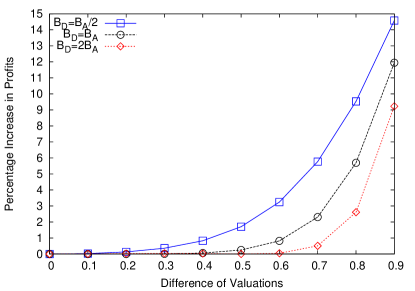
Figure 2: Percentage increase in profits for the incumbent (defender) vs the difference of valuations between communities ($\delta$) by committing to the Stackelberg leadership model versus Nash equilibrium.

In Figure 1, we observe that for small difference of valuations Stackelberg and Nash equilibria give roughly the same profit. However, when the difference of valuations increases we have that while the profit obtained by Stackelberg increases, the profit of the Nash equilibrium after a threshold decreases.

In Figure 2, we notice that for a small difference of valuations between communities, both models give roughly the same profits, however when the difference of valuations between communities grows, the Stackelberg equilibrium gives much higher profits than the Nash equilibrium.

Another interesting observations is that in the case when the defender has smaller budget compared with the attacker, the difference in profits from both equilibria is much higher compared with the scenario when the defender has higher budget.

6 Conclusions

We have studied the case of two marketing campaigns competing to maximize their profit from the network value of the potential customers. We have analyzed the following situations: (a) when the decision of how many resources to allocate to market to potential customers is made simultaneously, and (b) when the decision is sequential and the incumbent foreseeing the arrival of the challenger can commit to a strategy before its arrival.

Appendix

The term $x_{A}^{*}$ was computed through Matlab Symbolic Toolbox from the equation:

$$x=-\frac{B_{D}}{m}\frac{\alpha x}{(\alpha-\beta)x+\beta B_{A}/m}+\frac{B_{A}+B_{D}}{m}\frac{\sqrt{\alpha x}}{\sqrt{\alpha x}+\sqrt{\beta(B_{A}/m-x)}},$$

and it is given by

$$x_{A}^{*}=(((3^{(1/2)}((B_{D}^{2}\alpha^{8}\beta^{2}(4B_{A}^{4}\alpha^{4}+8B_{A}^{4}\alpha^{2}\beta^{2}+4B_{A}^{4}\beta^{4}+4B_{A}^{3}B_{D}\alpha^{4}-8B_{A}^{3}B_{D}\alpha^{3}\beta+72B_{A}^{3}B_{D}\alpha^{2}\beta^{2}-8B_{A}^{3}B_{D}\alpha\beta^{3}$$

$$+4B_{A}^{3}B_{D}\beta^{4}-B_{A}^{2}B_{D}^{2}\alpha^{4}-24B_{A}^{2}B_{D}^{2}\alpha^{3}\beta+146B_{A}^{2}B_{D}^{2}\alpha^{2}\beta^{2}-24B_{A}^{2}B_{D}^{2}\alpha\beta^{3}-B_{A}^{2}B_{D}^{2}\beta^{4}-16B_{A}B_{D}^{3}\alpha^{3}\beta+96B_{A}B_{D}^{3}$$

$$\alpha^{2}\beta^{2}-16B_{A}B_{D}^{3}\alpha\beta^{3}+4B_{D}^{4}\alpha^{3}\beta+8B_{D}^{4}\alpha^{2}\beta^{2}+4B_{D}^{4}\alpha\beta^{3}))/(m^{6}(\alpha^{2}-\beta^{2})^{4}))^{(1/2)})/18-(\alpha^{3}(2B_{A}\beta^{2}-B_{A}\alpha^{2}+3B_{A}\alpha\beta$$

$$+4B_{D}\alpha\beta)^{3})/(27m^{3}(\alpha+\beta)^{3}(\alpha-\beta)^{3})+(\alpha^{3}\beta(2B_{A}\beta^{2}-B_{A}\alpha^{2}+3B_{A}\alpha\beta+4B_{D}\alpha\beta)(3B_{A}^{2}\alpha\beta-2B_{A}^{2}\alpha^{2}+B_{A}^{2}\beta^{2}$$

$$-2B_{A}B_{D}\alpha^{2}+6B_{A}B_{D}\alpha\beta+B_{D}^{2}\alpha^{2}+B_{D}^{2}\alpha\beta))/(6m^{3}(\alpha+\beta)^{2}(\alpha-\beta)^{3})$$

$$+(B_{A}\alpha^{4}\beta^{2}(B_{A}+B_{D})^{2})/(2m^{3}(\alpha+\beta)(\alpha-\beta)^{2}))^{(1/3)}-(\alpha(2B_{A}\beta^{2}-B_{A}\alpha^{2}+3B_{A}\alpha\beta+4B_{D}\alpha\beta))/(3m(\alpha^{2}-\beta^{2}))$$

$$+(\alpha^{2}(B_{A}^{2}\alpha^{4}+2B_{A}^{2}\alpha^{2}\beta^{2}+B_{A}^{2}\beta^{4}-2B_{A}B_{D}\alpha^{3}\beta+12B_{A}B_{D}\alpha^{2}\beta^{2}-2B_{A}B_{D}\alpha\beta^{3}-3B_{D}^{2}\alpha^{3}\beta+10B_{D}^{2}\alpha^{2}\beta^{2}$$

$$-3B_{D}^{2}\alpha\beta^{3}))/(9m^{2}(\alpha^{2}-\beta^{2})^{2}((3^{(1/2)}((B_{D}^{2}\alpha^{8}\beta^{2}(4B_{A}^{4}\alpha^{4}+4B_{A}^{4}\beta^{4}+4B_{A}^{3}B_{D}\alpha^{4}+4B_{A}^{3}B_{D}\beta^{4}+4B_{D}^{4}\alpha\beta^{3}+4B_{D}^{4}\alpha^{3}\beta$$

$$-B_{A}^{2}B_{D}^{2}\alpha^{4}-B_{A}^{2}B_{D}^{2}\beta^{4}+8B_{A}^{4}\alpha^{2}\beta^{2}+8B_{D}^{4}\alpha^{2}\beta^{2}+146B_{A}^{2}B_{D}^{2}\alpha^{2}\beta^{2}-16B_{A}B_{D}^{3}\alpha\beta^{3}-16B_{A}B_{D}^{3}\alpha^{3}\beta-8B_{A}^{3}B_{D}\alpha\beta^{3}$$

$$-8B_{A}^{3}B_{D}\alpha^{3}\beta+96B_{A}B_{D}^{3}\alpha^{2}\beta^{2}-24B_{A}^{2}B_{D}^{2}\alpha\beta^{3}-24B_{A}^{2}B_{D}^{2}\alpha^{3}\beta+72B_{A}^{3}B_{D}\alpha^{2}\beta^{2}))/(m^{6}(\alpha^{2}-\beta^{2})^{4}))^{(1/2)})/18$$

$$-(\alpha^{3}(2B_{A}\beta^{2}-B_{A}\alpha^{2}+3B_{A}\alpha\beta+4B_{D}\alpha\beta)^{3})/(27m^{3}(\alpha+\beta)^{3}(\alpha-\beta)^{3})$$

$$+(\alpha^{3}\beta(2B_{A}\beta^{2}-B_{A}\alpha^{2}+3B_{A}\alpha\beta+4B_{D}\alpha\beta)(B_{A}^{2}\beta^{2}-2B_{A}^{2}\alpha^{2}+B_{D}^{2}\alpha^{2}-2B_{A}B_{D}\alpha^{2}+$$

$$3B_{A}^{2}\alpha\beta+B_{D}^{2}\alpha\beta+6B_{A}B_{D}\alpha\beta))/(6m^{3}(\alpha+\beta)^{2}(\alpha-\beta)^{3})+(B_{A}\alpha^{4}\beta^{2}(B_{A}+B_{D})^{2})/(2m^{3}(\alpha+\beta)(\alpha-\beta)^{2}))^{(1/3)}))/\alpha.$$

References

• [1] P. Domingos and M. Richardson, “Mining the network value of customers,” in Proceedings of the 7th ACM SIGKDD International Conference on Knowledge Discovery and Data Mining, (New York), pp. 57–66, ACM Press, Aug. 26–29 2001.
• [2] M. Richardson and P. Domingos, “Mining knowledge-sharing sites for viral marketing,” in Proceedings of the 8th ACM SIGKDD International Conference on Knowledge Discovery and Data Mining, (New York), pp. 61–70, ACM Press, July 23-26 2002.
• [3] G. Nemhauser, L. Wolsey, and M. Fisher, “An analysis of approximations for maximizing submodular set functions I,” Mathematical Programming, vol. 14, no. 1, pp. 265–294, 1978.
• [4] D. Kempe, J. Kleinberg, and É. Tardos, “Maximizing the spread of influence through a social network,” in Proceedings of the 9th ACM SIGKDD International Conference on Knowledge Discovery and Data Mining, (New York), pp. 137–146, ACM Press, Aug. 24–27 2003.
• [5] D. Kempe, J. Kleinberg, and É. Tardos, “Influential nodes in a diffusion model for social networks,” in ICALP: Annual International Colloquium on Automata, Languages and Programming, 2005.
• [6] Mossel and Roch, “On the submodularity of influence in social networks,” in STOC: ACM Symposium on Theory of Computing (STOC), 2007.
• [7] P. Clifford and A. Sudbury, “A model for spatial conflict,” Biometrika, vol. 60, no. 3, pp. 581–588, 1973.
• [8] R. A. Holley and T. M. Liggett, “Ergodic theorems for weakly interacting infinite systems and the voter model,” The Annals of Probability, vol. 3, no. 4, pp. 643–663, 1975.
• [9] E. Even-Dar and A. Shapira, “A note on maximizing the spread of influence in social networks,” in Proceedings of the 3rd International Conference on Internet and Network Economics (WINE’07), (Berlin, Heidelberg), pp. 281–286, Springer-Verlag, 2007.
• [10] S. Bharathi, D. Kempe, and M. Salek, “Competitive influence maximization in social networks,” in Internet and Network Economics (X. Deng and F. Graham, eds.), vol. 4858 of Lecture Notes in Computer Science, pp. 306–311, Springer Berlin Heidelberg, 2007.
• [11] J. Goldenberg, B. Libai, and E. Muller, “Talk of the network: A complex systems look at the underlying process of word-of-mouth,” Marketing Letters, vol. 12, no. 3, pp. 211–223, 2001.
• [12] S. Goyal and M. Kearns, “Competitive contagion in networks,” in Proceedings of the 44th Symposium on Theory of Computing, STOC ’12, (New York, NY, USA), pp. 759–774, ACM, 2012.
• [13] A. Borodin, Y. Filmus, and J. Oren, “Threshold models for competitive influence in social networks,” in Proceedings of the 6th International Conference on Internet and Network Economics, WINE’10, (Berlin, Heidelberg), pp. 539–550, Springer-Verlag, 2010.
• [14] G. C. Chasparis and J. Shamma, “Control of preferences in social networks,” in Proceedings of the 49th IEEE Conference on Decision and Control (CDC), pp. 6651–6656, Dec 2010.
• [15] O. Gross and R. Wagner, “A continuous colonel blotto game,” in RAND Corporation RM-408, 1950.
• [16] B. Roberson, “The colonel blotto game.,” Economic Theory, vol. 29, no. 1, pp. 1 – 24, 2006.
• [17] A. M. Masucci and A. Silva, “Strategic Resource Allocation for Competitive Influence in Social Networks,” in Annual Allerton Conference on Communication, Control, and Computing, (Monticello, Illinois, United States), Oct. 1–3 2014.
• [18] G. Schwartz, P. Loiseau, and S. Sastry, “The heterogeneous Colonel Blotto Game,” in NETGCOOP 2014, International Conference on Network Games, Control and Optimization, October 29-31, 2014,, (Trento, Italy), 2014.
• [19] R. Powell, “Sequential, nonzero-sum “blotto”: Allocating defensive resources prior to attack,” Games and Economic Behavior, vol. 67, no. 2, pp. 611 – 615, 2009.
• [20] L. Friedman, “Game-theory models in the allocation of advertising expenditures,” Operations Research, vol. 6, no. 5, pp. 699–709, 1958, http://pubsonline.informs.org/doi/pdf/10.1287/opre.6.5.699.