Almost Optimal Energy-Efficient Cognitive Communications in Unknown Environments

Pan Zhou, Member, IEEE, Chenhui Hu, Student Member, IEEE, Tao Jiang, Senior Member, IEEE, Dapeng Wu, Fellow, IEEE
Abstract

Cognitive (Radio) (CR) Communications (CC) are mainly deployed within the environments of primary (user) communications, where the channel states and accessibility are usually stochastically distributed (benign or IID). However, many practical CC are also exposed to disturbing events (contaminated) and vulnerable jamming attacks (adversarial or non-IID). Thus, the channel state distribution of spectrum could be stochastic, contaminated or adversarial at different temporal and spatial locations. Without any a priori, facilitating optimal CC is a very challenging issue. In this paper, we propose an online learning algorithm that performs the joint channel sensing, probing and adaptive channel access for multi-channel CC in general unknown environments. We take energy-efficient CC (EECC) into our special attention, which is highly desirable for green wireless communications and demanding to combat with potential jamming attack who could greatly mar the energy and spectrum efficiency of CC. The EECC is formulated as a constrained regret minimization problem with power budget constraints. By tuning a novel exploration parameter, our algorithms could adaptively find the optimal channel access strategies and achieve the almost optimal learning performance of EECC in different scenarios provided with the vanishing long-term power budget violations. We also consider the important scenario that cooperative learning and information sharing among multiple CR users to see further performance improvements. The proposed algorithms are resilient to both oblivious and adaptive jamming attacks with different intelligence and attacking strength. Extensive numerical results are conducted to validate our theory.

Index Terms:
Energy Efficiency, Cognitive Radio, Online learning, Jamming attack and Multi-armed bandits

I Introduction

Cognitive (Radio) (CR) Communications (CC) are widely recognized as one of the promising Information and Communication technology (ICT) to release the tension of current spectrum-scarcity issue. Meanwhile, as growing explosively, ICT is playing a more and more important role in global greenhouse gas emissions, the energy-consumption of which contributes to $3$ percent of the worldwide electric energy consumption nowadays [1]. Thus, Energy-Efficient (EE) CC (EECC) has received great attention from the research community in recent years [2]. Admittedly, the joint design of channel sensing, probing, and accessing (SPA) scheme with the consideration of energy efficiency (EE) is pivotal for CC. Stimulated by the recent appearance of smart CR devices with adaptive and learning abilities, modern CCs have raised very high requirements to its solutions, especially in complex environments, where accurate channel distributions and states can barely be modeled and acquired due to unpredictable Primary User Activity (PUA) [3] in Primary Communications (PC), behaviors of other CC, potential jamming attacks, and other distributing events frequently seen in practice. Thus, it is critical for CR devices to learn from the environments and keep a good balance of allocating its transmission power wisely to achieve the goal of energy-efficiency and of designing almost optimal channel access schemes to reach the goal of spectrum-efficiency in EECC.

Undoubtedly, the communication model has a great impact on the performance of CC. A great amount of works assume priorly known statistical information and have proposed deterministic channel states models, e.g., POMDP [7], and accessibility models, e.g., Poisson Modeling of PUA [8] to make good approximations in benign wireless environments. Clearly, they are not suitable for complex or even unknown environments. To cope with the problem, a fairly reasonable and realistic line of studies assume no statistical prior information about the channel states and accessibility. Thus, online learning based methods (e.g., reinforcement learning (RL) [40]) are desirable to be adopted, e.g., [13] [21][22][26]. Within this context, the use of the Multi-armed bandit (MAB) theory [20] is highly identified over other learning approaches.

In summary, these works assume that the nature of CC environments is either stochastic (benign), where the channel state and accessibility are stochastically distributed [26] (IID), or adversarial[21] [22], where they can vary arbitrarily (adversarial or non-IID) by jamming attackers or adversarial UPA, etc. Respectively, these works are mainly categorized into two MAB models, namely, stochastic MAB [10, 11, 12] with IID assumption and adversarial MAB [21][22] with non-IID assumption. Accordingly, the analytical approaches and results for the two models are distinctively different. Note that the learning performance is qualified by the classic term “regret”, i.e., the performance difference between the proposed learning algorithm and the optimal one known in hindsight. A well-known fact is that stochastic MAB and adversarial MAB have the respective optimal regrets $O(log(n))$ [18] and $O(\sqrt{n})$ [19] over time $n$. Obviously, the stochastic MAB highly outperform that of the adversarial MAB in learning of convergence to the optimal strategies.

However, all related works [10, 11, 12] [21, 22, 23, 24, 25, 26, 27, 28] still rely on the priori of either the stochastic or the adversarial assumption, which is limited in describing practical CC environments. Because, the nature of the practical CC environments are not restricted to these two types and it usually can not be known in advance. On the one hand, consider a CC under potential jamming attack. Since the number and locations of jamming regions are often unrevealed, it is uncertain which regions may (or may not) suffer from the attack. Thus, the usual mind of applying adversarial MABs models [21][22] on all channels will lead to large values of regret, since a great portion of channels can still be stochastically distributed, while applying the stochastic MABs models is not feasible due to the existence of adversaries.

On the other hand, the stochastic MAB model [23][24, 26, 28][27] will face practical implementation issues. In almost all CC systems, the commonly seen occasionally disturbing events would make the stochastic channel distributions contaminated. These include the burst movements of individuals, the spectrums handoff and mobility [3] among users of PC and CC, and the jitter effects of electronmagnetic waves, etc. In this case, the channel distribution will not follow an IID process for a small portion of time. Thus, it is not clear to us whether the stochastic MAB is still applicable, how the contamination affects the learning performance and to what extent the contamination is negligible. Therefore, the design of a unified SPA scheme without any prior knowledge of the operating environment is very challenging. It is highly desirable and bears great theoretical value.

In this paper, we propose a novel adaptive multi-channel SPA algorithm for EECC that achieves almost optimal learning performance without any a priori of the CC environments. Importantly, we take EE into our special consideration with power budget constraints on each of the multi-channel access strategy. As such, our work can be regarded as the first work for the EECC in unknown environments, where optimal strategies can be gradually learned. Our innovative SPA scheme is based on the famous EXP3 [33] algorithm in the non-stochastic MAB with three main features: 1) We introduce a new control parameter into the exploration probability for each channel to facilitate automatically detection of the feature of environments; 2) we use and design the Lagrangian method delicately to model the the power budget constraints for our own EECC problem; 3) By joint control of learning rate and exploration probability, the proposed algorithm achieves almost optimal learning performance in different regimes with vanishing (sublinear) long-term power budget violations. Our main contributions are summarized as follows.

1) We define an appropriate EE model that is suitable for SPA scheme-based EECC over large spectrum pools and with fairness considerations. We categorize the features of the EECC environments mainly into four typical regimes, each of which are proved to achieve the almost optimal regret bounds with sublinear long-term power budget violations. Our proposed algorithm neither need to distinguish the type of PC, other CC and adversarial (jamming) behaviors, nor need to know the channel accessibility and quality within all the different features of the complex environments. Thus, it provides a complete solution for practical CC in general unknown environment.

2) The proposed AOEECC-EXP3++ algorithm considers information sharing of channels that belong to different channel access strategies, which can be regarded as a special type of combinatorial semi-bandit111The term first appears in [38], which is the combinatorial version of the classic MAB problems. problem. In this case, given the size of all channels $K$ and the number of transmitting channels $k$, the AOEECC-EXP3++ algorithm has the optimal tight regret bounds in both the adversarial settings [38] and the stochastic settings [37], which indicates the good scalability for different size of CC systems.

3) This work is also the first MAB-based constrained regret minimization (optimization) framework for CC in unknown environments in the online learning setting. Our proposed algorithms have polynomial time implementations, which result in good computational efficiency in practice.

4) We propose a novel cooperative learning algorithm that considers information sharing among multiple users of the CC systems to accelerating the learning speed of each individual users, which is desirable for the widely acknowledged feature of CC systems with cooperative spectrum sensing and sharing schemes [3]. It further improves the energy-efficiency and spectrum-efficiency of the EECC within a fixed time period.

5) We conduct plenty of diversified experiments based on real experimental datasets. Numerical results demonstrate that all advantages of the proposed algorithms are real and can be implemented easily in practice.

The rest of this paper is organized as follows: Section II discusses Related works. Section III describes the problem formulation. Section IV introduces the distributed learning algorithm, i.e, AOEECC. The performance results are presented in Section V. The multi-user cooperative learning algorithm is discussed in Section VI. Proofs of previous sections are in Section VII and Section VIII. Simulation results are available in Section IX. The paper is concluded in Section X.

II Related Works

Recently, online learning approach to address the dynamic channel access (DSA) problem in CC with less prior channel statistical information have received more and more attention than classic deterministic model approaches, e.g. channel states [7] and accessibility modeling [8]. The characteristics of repeated interactions with environments are usually categorized into the domain of RL [40], e.g. DSA by RL [13], anti-jamming CC by RL [14, 15, 16, 17]. It is worth pointing out that there exists extensive literature in RL, which is generally targeted at a broader set of learning problems in Markov Decision Processes (MDPs). The RL approach guarantees the performance asymptotically to infinite. Hence, it is not quite suitable for mission-critical advanced applications of CC, which is commonly seen in next generation wireless communications. By contrast, MAB problems constitute a special class of MDPs, for which the no-regret learning framework is generally viewed as more effective in terms of fast convergence time, finite-time optimality guarantee [39], and low computational complexity. Moreover, it has the inherent capability in keeping a good balance between “exploitation” and “exploration”. Thus, the use of MAB models is highly identified.

The works based on the stochastic MAB model often consider about the stochastically distributed channels in benign environments, such as [23][24][26, 27, 28][36]. The adversarial MAB model is applied to adversarial channel conditions, such as the anti-jamming CC [21][22]. In the machine learning society, the stochastic and adversarial MABs have co-existed in parallel for almost two decades. Only until recently, the first practical algorithm for both stochastic and adversarial bandits is proposed in [35] for the classic MAB problem. The current work uses the idea of introducing a novel exploration parameter [35]. But our focus is on the much harder combinatorial semi-bandit problem that needs to exploit the channel dependency among different SPA strategies, which is a nontrivial task. Moreover, our introducing of the Lagrangian method into the online EECC problem leads to an important finding that we need to set the learning rate and exploration probability together and the same for all regimes (as we defined) rather than could be adjusted separately for stochastic and adversarial regimes in [35]. This phenomenon indicates that the online learning for the EECC in unknown environments is a harder problem than classic regret minimization without constraints [21][22] [35].

The topic of EECC has recently received great attention in wireless communications society [2] due to the stimulation of green communications for ICT. The spectrum efficiency and energy efficiency are the two critical concerns. Almost all of them consider about deterministic channel state and accessibility models [42, 43, 44, 45, 46, 47] for DSA in CC. Some of the works try to achieve the spectrum efficiency [43], energy efficiency [42], while others try to achieve both goals [44, 45, 46, 47]. Being worthy of mention, there are a small amount of works focus only on optimization of the EE for spectrum sensing part[48] [50] within the whole CC circle. This part of energy cost is comparatively minor in scales when compare to circuit and transmission energy cost [3], which can be categorized into the circuit and processing energy cost as in classic wireless communications [5].

Recently works [18] [19] have used the exponential weights (similar to EXP3) MAB model to study the no-regret (sublinear) online learning for the EE of OFDM and MIMO-OFDM wireless communications. However, the problems are different from the EECC, and the dynamic channel evolution process is only assumed to be adversarial. Thus, our work is the first SPA scheme for EECC in general unknown environments that targets on both spectrum efficiency and energy efficiency without any deterministic channel model assumption.

III Problem Formulation

III-A Cognitive Communication Model

We first focus on EECC from the perspective of a single CR user (or called “secondary user” (SU)), which is distributed or uncoordinated with other CR users. It is consisted by a pair of transmitter and receiver within the region of PC. The transmitter sends data packets to the receiver synchronically over time with classic slotted model. The wireless environment is highly flexible in dynamics, i.e., besides the most influential PUA of a number of $M$ PUs that affect the CC’s channels’ qualities (states) and accessibility, there are interference from other SU transceiver pairs, potential jamming attack and channel fading, etc, would make the environment to be generally unknown. During each timeslot, the SU transmitter selects multiple channels $k$ to transmit data to the receiver over a set $[K]=\{c_{1},c_{2},...,c_{f},...,c_{K}\}$ of $K$ available orthogonal channels with possibly different data rates across them. When a channel $c_{f}$ is occupied by primary user (PU), it is called as busy, otherwise, it is called idle. However, the busy (or idle) probability of PU is not unknown. There are a set $[L]=\{S_{1},S_{2},...,S_{u},...,S_{L}\}$ of $L$ SU transceiver pairs making contention or interfering power among each other. However, the behavior is transparent to a single SU $S_{u}$. W.l.o.g, if there are adversarial events, we ascribe them to be launched by one jammer who attacks the set or a subset of $K$ channels, where its attacking strategies are unrevealed. At each time $n$, the EE calculated from the allocated power and received data rate of the SU $u$ on channel $f$ is denoted by $g_{n,u}(f)$, $g_{n,u}(f)\in[0,M]$. We omit subscript $u$ if there is no confusion from context. Here constant $M$ is the maximum value of EE for all channels. W.l.o.g., we normalize $M=1$ as usual in the regret analysis.

We employ the classic energy detection method [3] for spectrum sensing, i.e., if the transmitting single strength is above a threshold, we regard the channel is busy or attacked, i.e., $g_{n}(f)=0$. Otherwise, CC are allowed and $g_{n}(f)$ is released for the frequency $f$ even though there are other potential PUs, jammers and CR users transmitting with low interfering power. Thus, our model is suitable for both spectrum overlay and spectrum underlay [3] schemes. We assume that each radio out of the $k$ radios on the SU transmitter needs time $n_{s}$ for sensing the status of a channel and time $n_{p}$ for probing its quality. The actual time depends on the technology and device: the typical values of $t_{s}$ is about 10$ms$ and $t_{p}$ is from 10$ms$ to 133$ms$ [9]. Let $t_{sp}=t_{s}+t_{p}$. When a channel $f\in[K]$ is idle, transmitter/reciever can only access it for at most $t_{a}$ time at most, so it can detect the return of a PU. In practice, $t_{a}$ has the typical value of 2$s$. Let ${\mathds{1}_{n}}(f)$ be the indictor function that denote whether the SU decides to transmit data using the probed channel $c_{{\mathds{1}_{n}}(f)}$.

III-B Preliminary in EECC with Deterministic CSI

Before the discussion of our own problem, let us first review the classic EECC with deterministic channel accessibility and states. For the multi-channel CC, SUs only know its own payoff and strategy for each channel $f$ at timslot $t$, i.e., the realized transmission rate ${r_{t}}(f)$ and transmission power $\textsf{P}_{t}(f)$. At each timeslot $t$, each SU chooses a subset of channels over $n$ according to some sensing/probing rules, where the multi-channel access strategy is denoted by $i$ and we have $f\in i\subset S$. the transmission power for each channel is $\textsf{P}_{t}(i_{f}),1\leq i_{f}\leq k,1\leq i\leq N$, and the total transmission power over a strategy $i$ is $\textsf{P}_{t}(i)$, and $\textsf{P}_{t}(i)=\sum\nolimits_{f=1}^{k}{{\textsf{P}_{t}}(i_{f})}$. Then, the instant data transmission rate $r_{t}(f)$ for the SU at each selected channel $f$ is given as

$\displaystyle\begin{array}[]{l}\!\!{r_{t}}(f)\!=\!W{\log_{2}}(1\!+\!\vartheta{\textsf{SINR}}({\textsf{P}_{t}}))=W\cdot{\mathds{1}_{t}}(f)\cdot\\ \!\!\!{\log}\left(\!\!1\!+\!\frac{{\vartheta{\textsf{P}_{t}}(f){g_{ff}}(s_{t}^{f})}}{{\underbrace{\sum\limits_{j\neq f}^{f\in K}{{\textsf{P}_{t}}(j){g_{fj}}(s_{t}^{j})}}_{other\ CRs}\!+\!\underbrace{\sum\limits_{l=1}^{M}{b_{t}^{fl}\psi_{t}^{{}_{fl}}}}_{PUs}\!+\!\underbrace{{a_{t}^{fJ}\varpi_{t}^{{}_{fJ}}}}_{Jamming}\!+\!\underbrace{(\sigma^{f}_{t})^{2}}_{noise}}}\!\!\right),\end{array}$

where ${g_{ff}}(s_{t}^{f})$ and ${g_{fj}}(s_{t}^{j})$ are the respective channel gains from itself and other SUs with instant channel states$s_{t}^{f}$ and $s_{t}^{j}$, $b_{t}^{f}$ and $\psi_{t}^{{}_{fl}}$ are the respective interfering power and channel gain from the PU $l$, $a_{t}^{f}$ and $\varpi_{t}^{{}_{fa}}$ are the respective interfering power and channel gain from the jammer $J$, and $(\sigma^{f}_{t})^{2}$ is the background noise power. The unit of $r_{t}(f)$ is $nats/s$.

In traditional wireless communications, the EE of the multi-channel or OFDM (e.g. [5][18]) wireless systems with the number of subchannel (subcarrier) $k$ at timeslot $t$ is defined as

$\displaystyle\quad\quad\textup{EE}_{t}=\frac{{\sum\nolimits_{f=1}^{k}{{r_{t}}(i_{f})}}}{{\textsf{P}_{c}^{t}(i)+\sum\nolimits_{f=1}^{k}{{\textsf{P}_{t}}(i_{f})}}}\quad nats/J,$ (2)

where $P_{c}^{t}$ is the processing and circuit power consumption at time $t$ while ${{\textsf{P}_{t}}(i_{f})}$ is the transmission power for each sub-channel (sub-carrier) $f$.

By contrast, the definition of EE in EECC is slightly different. Because the multi-channel CC is not restricted to a pre-defined fixed set of OFDM (OFDMA) channel sets, where multi-radio based spectrum sensing and channel probing are necessary to scan from a large spectrum pool separately for a group of (potentially) nonconsecutive and distributed channels with the best channel sensing/probing qualities for general CC systems [6]. As such, the measurement of EE for EECC is from the view of each sensed/probed transmitting channel within the SPA scheme, i.e.,

$\displaystyle\quad\quad\textup{EE}_{t,f}=\frac{{{r_{t}}(i_{f})}}{{\textsf{P}_{c}^{t}(i_{f})+{{\textsf{P}_{t}}(i_{f})}}}\quad nats/J.$ (3)

Then, the overall average EE for the each SPA strategy $i$ is given as

$\displaystyle\quad\quad\textup{EE}_{t}^{CC}=\frac{1}{k}\sum\nolimits_{f=1}^{k}\textup{EE}_{t,f}\quad nats/J,\forall f\in i.$ (4)

Note that the sensing and probing energy consumption are also categorized into $P_{c}^{t}(i_{f})$ with $\sum\nolimits_{f=1}^{k}P_{c}^{t}(i_{f})=\textsf{P}_{c}^{t}(i)$222 More precisely, we could divide the circuit and processing power among the $k$ channels according to the bandwidth of each channel and calculate the sensing and probing energy cost based on the monitoring of each channel. Roughly speaking, we can simply do an energy-cost division among all channels $k$. and $\sum\nolimits_{f=1}^{k}{{\textsf{P}_{t}}(i_{f})}={{\textsf{P}_{t}}(i)}$. A simple fact about the relation of (2) and (4) is that $\max_{f}\textup{EE}_{t}^{CC}(f)\geq\textup{EE}_{t}^{CC}\geq\textup{EE}_{t}\geq\min_{f}\textup{EE}_{t}^{CC}(f)$. When $\forall f=f^{\prime}$, $\textup{EE}_{t,f}=\textup{EE}_{t,f^{\prime}}$, $\textup{EE}_{t}^{CC}=\textup{EE}_{t}$. Thus, maximize $\textup{EE}_{t}^{CC}$ will push the fairness of EE among different channels. Incorporated with sensing and probing, and after determined the channel access strategy $i$, the EECC can be formulated as the following nonlinear program.

$\displaystyle\begin{array}[]{l}\quad\max\quad\quad\quad\ \textup{EE}_{t}^{CC}\\ \emph{subject to}\quad\textsf{P}_{t}(i)\leq{{\textsf{P}}_{o}},\end{array}$

where each SU has a power budget  $\textsf{ P}_{o}$. By similar approaches in [5] that the problem (III-B) is also quasi-concave with respect to $\textsf{P}_{t}(i_{f})$, where water-filling method can be used to resolve the problem. Moreover, the definition of $\textup{EE}_{t}^{CC}$ enables the information sharing of $\textup{EE}_{t,f}$ for each channel among different strategies, which is specially suitable for EECC design over large spectrum pools.

III-C The Adaptive Online Learning for EECC: A Constrained Regret Minimization Formulation

In reality, since no secret is shared and no adversarial event is informed to the transceiver pair, the multi-channel EECC in unknown environments are necessary to sensing/probing and hoping among different channels to dynamically access a subset to maximize its accumulated EE over time. Namely, this sequential channel sensing/probing/accessing (SPA) problem is to determine when to conduct the channel hopping (multi-channel access) and power allocation repeated game with environments, without knowing instant channel states, for a pair of CR user transceiver so as to improve the EE of CC. The difference of our SPA problem (based on MAB) with the classic MAB problem is that, at every timeslot $t$, the classic MAB receives a reward and repeat this for $T$ timeslots; while for the SPA problem, at a timeslot $t$, we will not have any gain if the the CR users donot happen to use the channel for data transmission after the sense/probe of the channel.

To address this issue, we only need to count the timeslots spent for sensing/probing a chosen channel a round (Or still say “timeslot”, if no confusion). The immediate following timeslot spent for data transmission over a chosen multiple channel set are not counted as a round. However, we will calculate and treat the averaged EE (4) from (3) based on the previous transmitted data and the chosen transmission power and known circuit and processing power $\textsf{P}_{c}^{t}(i_{f})$ for each sensed/probed channel $f$, where its gain is ${g_{t}}(f)={\mathds{1}_{t}}(f)\cdot\frac{1}{{{Z_{t}}}}\int_{0}^{{Z_{t}}}{\textup{EE}_{t,f}}\cdot(1-{\Pr_{t}}(PU,J,SU))$, where $Z_{t}$ denotes the time of the actual transmission and ${\Pr_{t}}(PU,J,SU)$ are the probability that the transmission will be destroyed by the return of PU, jammer or some other SUs within the $Z_{t}$ time duration. We set that $t_{a}=Z_{t}$. Let $n$ be the number of sensing/probing timeslots executed during the whole run of the system evolution duration $T$, which should satisfy the condition $n\cdot{t_{sp}}+\sum\nolimits_{t=1}^{n}{{\mathds{1}_{t}}(i)}\cdot{Z_{t}}\leq T.$ The first part is the time spent for sensing/probing and the second part is the time spent for multi-channel EECC.

For the multi-channel accessing part, let us denote $\{0,1\}^{K}$ as the vector space of all $K$ channels. The strategy space for the transmitter is denoted as $S\subseteq\{0,1\}^{K}$ of size $N=\binom{K}{k}$. If the $f^{th}$-channel is selected for transmitting data, the value of the $f$-th entry of a vector (channel access strategy) is $1$, and 0 otherwise. In the case of the existence of jamming attack on a subset of $k_{j}$ channels, the strategy space for the jammer is denoted as $S_{j}\subseteq\{0,1\}^{K}$ of size $\binom{K}{k_{j}}$. For convenience, we say that the $f$-th channel is jammed if the value of $f$-th entry is 0 and otherwise is 1.

Formally, our MAB-based SPA problem is described as follows: at each timeslot $n=1,2,3,...$, the transmitter (as a decision maker) selects a strategy $I_{n}$ from $S_{r}$ with a power strategy $\textsf{P}_{t}(I_{f}),\forall f\in I_{n}$. The cardinality of $S_{r}$ is $|S_{r}|=N$. The reward $g_{n}(f)$ is assigned to each channel $f\in\{1,...,K\}$ and the SU only gets rewards in strategy $i\in S_{r}$. The total reward of a strategy $i$ in timeslot $n$ is ${g_{n}(i)}=\sum\nolimits_{f\in i}{{g_{n}(f)}}$. Then, on the one hand, the cumulative reward (or EE) up to timeslot $n$ of the strategy $i$ is ${G_{n,i}}=\textup{EE}_{n}^{CC}=\sum\nolimits_{t=1}^{n}{{g_{t}(i)}}=\sum\nolimits_{f\in i}{\sum\nolimits_{t=1}^{n}{{g_{t}(f)}}}.$ On the other hand, the total reward over all the chosen strategies by the receiver up to timeslot $n$ is ${\hat{G}_{n}}=\hat{\textup{ EE}}_{n}^{CC}=\sum\nolimits_{t=1}^{n}{{g_{t}(I_{t})}}=\sum\nolimits_{t=1}^{n}{\sum\nolimits_{f\in{I_{t}}}{{g_{t}(f)}}}$, where the strategy $I_{t}$ is chosen randomly according to some distribution over $S_{r}$. The performance of this algorithm is qualified by regret $R(n)$, defined as the difference between the expected number of successfully received data packets using our proposed algorithm and the expected rewards that use the best fixed solution up to $n$, i.e.,

$\displaystyle R(n)=\mathop{\max}\limits_{i\in{S_{r}}}\mathbb{E}_{i\sim{\textbf{p}_{n}}}\{{{G_{n,i}}}\}-\mathbb{E}[{{{\hat{G}}_{n}}}],$ (6)

where $\textbf{p}_{n}$ is the decision probability vector over all strategies and the maximum is taken over all available strategies. However, if we use the gain (reward) model, we will face technical difficulties as presented in [20] (pages 25-28). Thus, we can introduce the loss model by the simple trick of $\ell_{n}(f)=1-g_{n}(f)$ for each channel $f$ and $\ell_{n}(i)=k-g_{n}(i)$ for each strategy to avoid this issue. Then, we have $L_{n}(i)=nk-G_{n,i}$ where ${L_{n}}(i)=\sum\nolimits_{t=1}^{n}\ell_{n}(i)={\sum\nolimits_{t=1}^{n}{\sum\nolimits_{f\in i}{{\ell_{t}(f)}}}}$, and similarly, we have $\hat{L}_{n}=nk-\hat{G}_{n}$. Use $\mathbb{E}_{n}[\cdot]$ to denote expectations on realization of all strategies as random variables up to round $n$, the expected regret $R(n)$ can be rewritten as

$\displaystyle\begin{array}[]{l}\!\!R(n)=\mathbb{E}\left[{\sum\limits_{t=1}^{n}{{\textbf{p}_{t}^{T}}{\ell_{t}}(i)-{\textbf{p}_{t}^{T}}{\ell_{t}}({I_{t}})}}\right]\\ \quad\quad=\mathbb{E}\left[{{{\hat{L}}_{n}}}\right]-\mathop{\min}\limits_{i\in{S_{r}}}\mathbb{E}_{i\sim{\textbf{p}_{n}}}\left\{{{L_{n}(i)}}\right\}\\ \quad\quad=\mathbb{E}[\sum\limits_{t=1}^{n}{\mathbb{E}_{t}[{\sum\limits_{f\in{I_{t}}}{{\ell_{t}(f)}}}]}]-\mathop{\min}\limits_{i\in{S_{r}}}({\mathbb{E}[{\sum\limits_{t=1}^{n}\mathbb{E}_{t}[{\sum\limits_{f\in i}{{\ell_{t}(f)}}}]}\!\!]}).\end{array}$

The goal of the algorithm is to minimize the weak regret [20], or simply called regret. For AOEECC, in addition to rewards, there are power budget constraints on the decision of transmission power $\textsf{P}_{t}(f)$ that need to be satisfied. Particularly, for the decision $\textbf{p}_{n}$ made by the learner for each channel access strategy, the power budget constraint can be written as

$\displaystyle\textbf{p}_{n}^{\textup{T}}\textsf{{P}}_{n}\leq\textsf{P}_{o}.$ (8)

Note that the SUs of the CC need to make decisions $\textbf{p}_{n}$ that attains maximal cummulative reward while satisfying the additional constraints (8).

Refer to caption
Figure 1: Multi-channel EECC in Different Regimes

Within our setting, we refer this problem as the constrained regret minimization problem. More precisely, let $\textbf{{P}}=\{\textsf{P}(1),...,\textsf{P}(N)\}$ be the constraint vector defined over power allocation actions. In stochastic setting, the vector $\mathcal{P}$ is not predetermined and is unknown to the learner. In each timeslot $t$, beyond the reward feedback, the SU receives a random realization $\textbf{{P}}_{t}=\{\textsf{P}_{t}(1),...,\textsf{P}_{t}(i),...,\textsf{P}_{t}(N)\}$ of $\mathcal{P}$, where $\mathbb{E}[{\textsf{P}_{t}(i)}]=\textsf{P}(i)$. W.l.o.g., we assume $\textsf{P}_{t}\in[0,1]^{N}$ and $\textsf{P}_{o}\in[0,1]$. Formally, the goal is to attain a gradually vanishing constrained regret as

$\displaystyle\textup{Regret}_{n}={R(n)}_{\textbf{p}_{n}^{\textup{T}}\textsf{P}}\leq O(n^{1-\beta_{1}}).$ (9)

Furthermore, the decision $\textbf{p}_{n}$ made by the learner are required to attain sublinear bound on the violation of the constraint in long run, i.e.,

$\displaystyle\textup{Violation}_{n}=\left[\sum\limits_{t=1}^{n}(\textbf{p}_{t}^{\textup{T}}\textsf{P}-\textsf{P}_{o})\right]_{+}\leq O(n^{1-\beta_{2}}).$ (10)

In contrast to the short-term constraints that the constraint (9) is required to be satisfied at every timeslot, SUs are allowed to violate the constraints for some rounds in a controlled way; but the constraints must hold on average for all rounds, i.e., $(\sum\nolimits_{t=1}^{n}\textbf{p}_{t}^{\textup{T}}\textsf{P})/n\leq\textsf{P}_{o}$.

III-D The Four Regimes of Wireless Environments

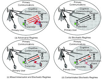
Since our algorithm does not need to know the nature of the environments, there exist different features of the environments that will affect the its performance. We categorize them into the four typical regimes as shown in Fig. 1.

III-D1 Adversarial Regime

In this regime, there is a jammer sending interfering power or injecting garbage data packets over all $K$ channels such that the transceiver’s channel rewards are completely suffered by an unrestricted jammer (See Fig.1 (a)). Usually, the EE will be significantly reduced in the adversarial regime. Note that, as a classic model of the well known non-stochastic MAB problem [33], the adversarial regime implies that the jammer often launches attack in every timeslot. It is the most general setting and other three regimes can be regarded as special cases of the adversarial regime.

Attack Model: Different attack philosophies will lead to different level of effectiveness. We focus on the following two type of jammers in the adversarial regime:

a) Oblivious attacker: an oblivious attacker attacks different channels with different attacking strength as a result of different EE reductions, which is independent of the past communication records it might have observed.

b) Adaptive attacker: an adaptive attacker selects its attacking strength on the targeted (sub)set of channels by utilizing its past experience and observation of the previous communication records. It is very powerful and can infer the SPR protocol and attack with different level of strength over a subset of channels during a single timeslot based on the historical monitoring records. As shown in a recent work, no bandit algorithm can guarantee a sublinear regret $o(t)$ against an adaptive adversary with unbounded memory, because the adaptive adversary can mimic the behavior of SPR protocol to attack, which leads to a linear regret (the attack can not be defended). Therefore, we consider a more practical $\theta$-memory-bounded adaptive adversary [29] model. It is an adversary constrained to loss functions that depends only on the $\theta+1$ most recent strategies.

III-D2 Stochastic Regime

In this regime, the SU’s transceiver communicating over $K$ stochastic channels within PC is shown in Fig.1 (b). The channel loss $\ell_{n}(f),\forall f\in 1,...,K$ (Obtained by transferring the reward to loss $\ell_{n}(f)=1-g_{n}(f)$) of each channel $f$ are sampled independently from an unknown distribution that depends on $f$, but not on $n$. We use $\mu_{f}=\mathbb{E}\left[{{\ell_{n}(f)}}\right]$ to denote the expected loss of channel $f$. We define channel $f$ as the best channel if $\mu(f)={\min_{f^{\prime}}}\{{\mu(f^{\prime})}\}$ and suboptimal channel otherwise; let $f^{*}$ denote some best channel. Similarly, for each strategy $i\in S_{r}$, we have the best strategy $\mu(i)={\min_{i^{\prime}}}\{{\sum\nolimits_{f\in i^{\prime}}{\mu(f)}}\}$ and suboptimal strategy otherwise; let $i^{*}$ denote some best strategy. For each channel $f$, we define the gap $\Delta(f)=\mu(f)-\mu({f^{*}})$; let $\Delta_{f}={\min_{f:\Delta(f)>0}}\left\{{\Delta(f)}\right\}$ denote the minimal gap of channels. Let $N_{n}(f)$ be the number of times channel $f$ was played up to time $n$, the regret can be rewritten as

$\displaystyle R(n)=\sum\nolimits_{f}{\mathbb{E}\left[{{N_{n}}(f)}\right]}\Delta(f).$ (11)

Note that we can calculate the regret either from the perspective of channels $f\in 1,...,K$ or from the perspective of strategies $i\in S_{r}$. However, because of the set of strategies is of the size $\binom{K}{k}$ that grows exponentially with respect to $K$ and it does not exploit the channel dependency among different strategies, we thus calculate the regret from channels, where tight regret bounds are achievable.

III-D3 Mixed Adversarial and Stochastic Regime

This regime assumes that the jammer only attacks $k_{j}$ out of $k$ currently chosen channels at each timeslot shown in Fig.1 (c). There is always a $k_{j}/k$ portion of channels under adversarial attack while the other $(k-k_{j})/k$ portion is stochastically distributed.

Attack Model: We consider the same attack model as in the adversarial regime. The difference here is that the jammer only attacks a subset of size $k_{j}$ over the total $k$ channels.

III-D4 Contaminated Stochastic Regime

The definition of this regime comes from many practical observations that only a few channels and timeslots are exposed to the jammer or other disturbing events in CC. In this regime, for the oblivious jammer, it selects some slot-channel pairs $(t,f)$ as “locations” to attack, while the remaining channel weights are generated the same as in the stochastic regime. We define the attacking strength parameter $\zeta\in[0,1/2)$. After certain $\tau$ timslots, for all $t>\tau$ the total number of contaminated locations of each suboptimal channel up to time $t$ is $t\Delta(f)\zeta$ and the number of contaminated locations of each best channel is $t\Delta_{f}\zeta$. We call a contaminated stochastic regime moderately contaminated, if $\zeta$ is at most $1/4$, we can prove that for all $t>\tau$ on the average over the stochasticity of the loss sequence the attacker can reduce the gap of every channel by at most one half.

Algorithm 1 AOEECC-EXP3++: An $\epsilon$-SPA Scheme for multi-channel EECC
  Input: $K,k,n$. See text for definition of $\eta_{n}$, $\xi_{n}(f)$, and $\delta_{n}$.
  Initialization: Set initial channel and strategy losses $\forall i\in[N],\tilde{L}_{0}(i)=0$ and $\forall f\in[K],\tilde{\ell}_{0}(f)=0$, respectively; Then the initial channel and strategy weights $\forall i\in[N],W_{0}(i)=k$ and $\forall f\in[K],w_{0}(f)=1$, respectively. The initial total strategy weight $W_{0}=N=\binom{K}{k}$. ​
  Set: ​​ $\beta_{n}\!\!=\!\!\frac{1}{2}\sqrt{\frac{{\ln K}}{{nK}}}$; ${\varepsilon_{n}}\left(f\right)\!=\!\min\left\{{\frac{1}{{2K}},{\beta_{n}},{\xi_{n}}\left(f\right)}\right\},\forall f\in\left[K\right]$ and $\gamma_{n}=\sum\nolimits_{f=1}^{K}{{\varepsilon_{n}}(f)}$.
  for  timeslot $n=1,2,...$ do
     1: Based on sensing and probing results, randomly selects a channel access strategy $I_{n}$ according to the strategy’t probability $p_{n}(i),\forall f\in\left[K\right]$, with $p_{n}(i)$ computed as follows:
$\displaystyle{p_{n}}(i)=\left\{\begin{array}[]{l}\!\!\!(1-\gamma_{n})\frac{{{w_{n-1}}\left(i\right)}}{{{W_{n-1}}}}+\!\sum\nolimits_{f\in i}{{\varepsilon_{n}}(f)}\ \emph{if}\ i\in\mathcal{C}\\ \!\!\!(1-\gamma_{n})\frac{{{w_{n-1}}\left(i\right)}}{{{W_{n-1}}}}\ \quad\quad\quad\quad\ \text{\emph{if}}\ i\notin\mathcal{C}\end{array}\right.$
     2: Computes the probability $q_{n}(f),\forall f\in\left[K\right]$,
$\displaystyle\begin{array}[]{l}{\rho_{n}}(f)=\sum\nolimits_{i:f\in i}{{p_{n}}(i)}=({1-\gamma_{n}})\frac{{\sum\nolimits_{i:f\in i}{{w_{n-1}}\left(i\right)}}}{{{W_{n-1}}}}\\ \quad\quad\quad\quad\quad\quad\quad\quad\ \ +\sum\nolimits_{f\in i}{{\varepsilon_{n}}(f)}\left|{\left\{{i\in\mathcal{C}:f\in i}\right\}}\right|.\end{array}$
     3: Sense and probe channels for $f\in{I_{n}}$. Receive the scaled (i.e., in the range $[0,1]$) loss model (converted from reward model) of reward and power , and then calculate EE for channel $f$, $\ell_{n-1}(f)$, and the realization of power budget ${\textsf{P}}_{n}(f)$, $\forall f\in I_{n}$. Update the estimated loss with augmented power allocation constraint $\tilde{\psi}_{n}(f),\forall f\in[K]$ as follows:
$\displaystyle{\tilde{\psi}_{n}}(f)=\left\{\begin{array}[]{l}{\mathbf{\tilde{\ell}}}_{n-1}(f)+\lambda_{n-1}\tilde{\textsf{P}}_{n-1}(f),\quad\text{\emph{if}}\ f\in{I_{n}}\\ 0\ \ \quad\quad\quad\quad\quad\quad\quad\quad\quad\quad\ \emph{otherwise}.\end{array}\right.$
     4: Update the Lagrangian Multiplier by the following equation:
$\displaystyle{\lambda_{n}}=[(1-\delta_{n-1}\eta_{n-1}\sqrt{\gamma_{n-1}}){\lambda_{n-1}}$
$\displaystyle\quad\quad\quad\quad\quad-\eta_{n-1}\sqrt{\gamma_{n-1}}(\textsf{P}_{o}-\textbf{p}_{n-1}^{\textup{T}}\tilde{\textsf{P}}_{n-1})]_{+}.$
     5: The receiver updates all the weights as
$\displaystyle{w_{n}}\left(f\right)={w_{n-1}}\left(f\right){e^{-\eta_{n}\tilde{\psi}_{n}(f)}}={e^{-\eta_{n}\tilde{\Psi}_{n}(f)}},$
$\displaystyle{{\bar{w}}_{n}}\left(i\right)=\prod\nolimits_{f\in i}{{w_{n}}(f)}={{\bar{w}}_{n-1}}\left(i\right){e^{-\eta_{n}{{\tilde{\psi}}_{n}}(i)}},$
The sum weights of all strategies is ${W_{n}}=\sum\nolimits_{i\in S_{r}}{{{\bar{w}}_{n}}\left(i\right)}$.
     6: Access each of the channel $f\in{I_{n}}$ with probability $\epsilon$, i.e., set ${\mathds{1}_{n}}(f)=1$ with probability $\epsilon$.
  end for

IV The AOEECC Algorithm

In this section, we focus on developing an AOEECC algorithm for the SU. The design philosophy is that the transmitter collects and learns the rewards of the previously chosen channels, based on which it can decide the next timeslot channel access strategy, i.e., the SU will decide whether to transmit data over the current channel set (called exploitation) or to continue sensing/probing some other channels for accessing (called exploration).

We describe the Algorithm 1, namely AOEECC-EXP3++, is a combinatorial variant based on EXP3 algorithm. Before we present the algorithm, let us introduce the following vectors: ${\bm{\tilde{\ell}}}_{t}$ is all zero vector except in the $I_{t}$th channel access strategy and so does the channel loss $\tilde{\mathbf{\ell}}_{t}(f)$ within the $I_{t}$, $\forall f\in I_{t}$, we have $\tilde{\mathbf{\ell}}_{t}(f)={\mathbf{\ell}}_{t}(f)/\rho_{n}(f)$. Similarly ${\bm{\tilde{}}{\textsf{P}}}_{t}$ is all zero vector except in $I_{t}$th channel access strategy and so does the power $\tilde{\textsf{P}}_{t}(f)$ within the $I_{t}$, $\forall f\in I_{n}$, where we have $\tilde{\textsf{P}}_{t}(f)={\textsf{P}}_{t}(f)/\rho_{n}(f)$. It is easy to verify $\mathbb{E}_{i_{t}}[{\mathbf{\tilde{\ell}}}_{t}(f)]={\mathbf{{\ell}}}_{t}(f)$ and $\mathbb{E}_{i_{t}}[\tilde{\textsf{P}}_{t}(f)]={\textsf{P}}_{t}(f)$, where $\bm{\rho}_{n,f}=(\rho_{n}(1),...,\rho_{n}(f),...,\rho_{n}(K))$ and $\textbf{p}_{n}=(p_{n}(1),...,p_{n}(i),...,p_{n}(N))$. In addition, we have the following equalities at step $5$ of Algorithm 1.

$\displaystyle\begin{array}[]{l}\!\!\!\!{{\tilde{\Psi}}_{n}}(f)={{\tilde{\Psi}}_{n-1}}(f)+{{\tilde{\psi}}_{n-1}}(f),{{\tilde{\Psi}}_{n}}(i)={{\tilde{\Psi}}_{n-1}}(i)+{{\tilde{\psi}}_{n-1}}(i)\\ \!\!\!\!{{\tilde{\Psi}}_{n}}(f)={{\tilde{L}}}_{n-1}(f)+\lambda_{n-1}{{\tilde{\Gamma}}_{n-1}}(f),\\ \!\!\!\!{{\tilde{\Psi}}_{n}}(i)={{\tilde{L}}}_{n-1}(i)+\lambda_{n-1}{{\tilde{\Gamma}}_{n-1}}(i),\\ \!\!\!\!{{\tilde{L}}_{n}}(f)={{\tilde{L}}_{n-1}}(f)+{{\tilde{\ell}}_{n-1}}(f),{{\tilde{L}}_{n}}(i)={{\tilde{L}}_{n-1}}(i)+{{\tilde{\ell}}_{n-1}}(i)\\ \!\!\!\!{{\tilde{\Gamma}}_{n}}(f)={{\tilde{{\Gamma}}}_{n-1}}(f)+{{\tilde{\textsf{P}}}_{n-1}}(f),{{\tilde{\Gamma}}_{n}}(i)={{\tilde{{\Gamma}}}_{n-1}}(i)+{{\tilde{\textsf{P}}}_{n-1}}(i)\\ \!\!\!\!{{\tilde{\ell}}_{n-1}}(i)=\sum\nolimits_{f\in i}{{{\tilde{\ell}}_{n-1}}(f)},{{\tilde{\textsf{P}}}_{n-1}}(i)=\sum\nolimits_{f\in i}{{{\tilde{\textsf{P}}}_{n-1}}(f)},\end{array}$

where ${{\tilde{L}}_{n}}(f)$ and ${{\tilde{\Gamma}}_{n}}(f)$ are the respective accumulated estimated loss and allocated power on channel $f$ up to round $n$, and ${{\tilde{L}}_{n}}(i)$ and ${{\tilde{\Gamma}}_{n}}(i)$ are the respective accumulated estimated loss and allocated power on strategy $i$ up to round $n$. Moreover, we have the exploration probability been decomposed for each channel, where we have $\gamma_{n}=\sum\nolimits_{f=1}^{K}{{\varepsilon_{n}}(f)}$.

Our new algorithm uses the fact that when losses (converted from rewards) and power of channels in the chosen strategy are revealed, it also shares this information with the common channels of the other chosen strategies. During each timeslot, we assign a channel weight that is dynamically adjusted based on the channel losses revealed. The weight of a strategy is determined by the product of weights of all channels. Our algorithm has two control levers: the learning rate $\eta_{n}$ and the exploration parameters $\xi_{n}(f)$ for each channel $f$. To facilitate the adaptive channel access to optimal solutions without the knowledge about the nature of the environments, the crucial innovation is the introduction of exploration parameters $\xi_{n}(f)$, which are tuned individually for each arm depending on the past observations.

A set of covering strategy is defined to ensure that each channel is sampled sufficiently often. It has the property that, for each channel $f$, there is a strategy $i\in\mathcal{C}$ such that $f\in i$. Since there are only $K$ channels and each strategy includes $k$ channels, we have $|\mathcal{C}|=\lceil{\frac{K}{{{k}}}}\rceil$. The value $\sum\nolimits_{f\in i}{{\varepsilon_{n}}(f)}$ means the randomized exploration probability for each strategy $i\in\mathcal{C}$, which is the summation of each channel $f$’s exploration probability ${\varepsilon_{n}}\left(f\right)$ that belongs to the strategy $i$. The introduction of $\sum\nolimits_{f\in i}{{\varepsilon_{n}}\left(f\right)}$ ensures that $p_{n}(i)\geq\sum\nolimits_{f\in i}{{\varepsilon_{n}}(f)}$ so that it is a mixture of exponentially weighted average distribution and uniform distribution [20] over each strategy.

In the following discussion, to facilitate the AOEECC-EXP3++ algorithm without knowing about the nature of environments, we can apply the two control parameters simultaneously by setting $\eta_{n}=\beta_{n}$, $2kK\eta\leq\delta=O(\eta_{n})$ and use the control parameter $\xi_{n}(f)$ such that it can achieve the optimal “root-n” regret in the adversarial regime and almost optimal “logarithmic-n” regret in the stochastic regime.

V Performance Results of EECC under $\epsilon$-SPA

This section analyzes the regret and power budget violation performance of our proposed AOEECC-EXP3++ algorithm in different regimes.

V-A Adversarial Regime

We first show that tuning $\eta_{n}$ and $\xi_{n}(f)$ together, we can get the optimal regret (of reward and violation) of AOEECC-EXP3++ in the adversarial regime, which is a general result that holds for all other regimes. Define ${{{\hat{G}}_{n}}}(\epsilon)$ as the expected average EEs that can be achieved by the $\epsilon$-SPA scheme over $n$ rounds. The Theorem 1, Theorem 3, Theorem 5, Theorem 7, Theorem 9 and Theorem 11 bound the regret of EE, $\mathop{\max}\nolimits_{i\in{S_{r}}}\mathbb{E}_{i\sim{\textbf{p}_{n}}}\{{{G_{n,i}}}\}-\mathbb{E}[{{{\hat{G}}_{n}}(1)}]$ when set $\epsilon=1$.

Theorem 1. Under the oblivious jamming attack, no matter how the status of the channels change (potentially in an adversarial manner), for $\eta_{n}=\beta_{n}$, $\delta_{n}=2k\sqrt{\frac{{K\ln K}}{n}}$ and any $\xi_{n}(f)=\tilde{O}(1/n)$, the regret of the AOEECC-EXP3++ algorithm for any $n$ satisfies:

$\displaystyle\begin{array}[]{l}\textup{Regret}_{n}={R(n)}_{\textbf{p}_{n}^{\textup{T}}\textsf{P}}\leq 4{k}\sqrt{nK\ln K}=O(n^{1/2}).\\ \textup{Violation}_{n}=\mathbb{E}{[{\sum\nolimits_{t=1}^{n}{\textbf{p}_{t}^{\textup{T}}\tilde{\textsf{P}}_{t}-\textsf{P}_{o}}}]_{+}}\leq O(n^{\frac{3}{4}}).\end{array}$

From Theorem 1, we can find that the regret is order and leading factor optimal when compared to the results in the anti-jamming wireless communications [25]. For the power budget violation, we have a regret of sublinear $O(n^{\frac{3}{4}})$. From the proof of the Theorem, this upper bound may be very loose.

According to the $\epsilon$-SPA scheme, CR user will transmit $\epsilon n$ times in expectation during $n$ rounds. It is easy to show $\mathbb{E}[{{\hat{G}}_{n}}(\epsilon)]=\epsilon\mathbb{E}[{{\hat{G}}_{n}}(1)]$, which implies $\mathbb{E}[{{\hat{G}}_{n}}(\epsilon)]\geq\epsilon\mathop{\max}\nolimits_{i\in{S_{r}}}\mathbb{E}[{{\hat{G}}_{n,i}}]-4\epsilon k\sqrt{nK\ln K}$. Let $G_{\max}$ be the large expected data rate of channel access strategies among all the strategies. We have $\mathop{\max}\nolimits_{i\in{S_{r}}}\mathbb{E}_{i\sim{\textbf{p}_{n}}}\{{{G_{n,i}}}\}=n\cdot G_{\max}$. Assume $t_{a}=\alpha t_{sp}$ where constant $\alpha\gg 1$. Then we have

Theorem 2. The expected EE of $\epsilon$-SPA scheme of AOEECC-EXP3++ in the adversarial regime under the oblivious jammer is at least

$\displaystyle\frac{{{{\hat{G}}_{n}}(\epsilon){t_{a}}}}{T}\!\geq\!\frac{{{G_{\max}}\!-\!4k\sqrt{\frac{{K\ln K}}{n}}}}{{\frac{1}{{\alpha\epsilon}}\!+\!1}}\!=\!\frac{{{G_{\max}}\!-\!4k\sqrt{\frac{{(1\!+\!\alpha\epsilon){t_{sp}}K\ln K}}{T}}}}{{\frac{1}{{\alpha\epsilon}}\!+\!1}},$

where $T=n{t_{sp}}+\epsilon n{t_{a}}$.

We find that when $T$ is sufficiently large, the achievable expected EE is at least $\frac{{{G_{\max}}}}{{\frac{1}{{\alpha\epsilon}}+1}}$, which is maximized when $\epsilon=1$. Obviously, the expected EE that can be achieved is no more than $\frac{{{G_{\max}}{t_{a}}}}{{{t_{sp}}+{t_{a}}}}=\frac{{{G_{\max}}}}{{\frac{1}{\alpha}+1}}$, because each transmission takes at least $t_{sp}+t_{a}$ time while the expected EE is no more than $G_{\max}$. Thus, when $T$ is sufficiently large, the $\epsilon$-SPA scheme of AOEECC-EXP3++ is almost optimal. Similar conclusions holds also for the following Theorem 4, Theorem 6, Theorem 8, Theorem 10, Theorem 12 and Theorem 14.

Theorem 3. Under the $\theta$-memory-bounded adaptive jamming attack, for $\eta_{n}=\beta_{n}$, $\delta_{n}=2k\sqrt{\frac{{K\ln K}}{n}}$ and any $\xi_{n}(f)\geq 0$, the regret of the AOEECC-EXP3++ algorithm for any $n$ is upper bounded by:

$\displaystyle\begin{array}[]{l}\textup{Regret}_{n}={R(n)}_{\textbf{p}_{n}^{\textup{T}}\textsf{P}}\leq O((\theta+1){(4{k}\sqrt{K\ln K})^{\frac{2}{3}}}{n^{\frac{2}{3}}}).\\ \textup{Violation}_{n}=\mathbb{E}{[{\sum\nolimits_{t=1}^{n}{\textbf{p}_{t}^{\textup{T}}\tilde{\textsf{P}}_{t}-\textsf{P}_{o}}}]_{+}}\leq O(n^{\frac{3}{4}}).\end{array}$

Theorem 4. The expected EE of $\epsilon$-SPA scheme of AOEECC-EXP3++ in the adversarial regime under the $\theta$-memory-bounded adaptive jammer is at least

$\displaystyle\frac{{{{\hat{G}}_{n}}(\epsilon){t_{a}}}}{T}\!\geq\!\frac{{{G_{\max}}\!-\!(\theta+1){{({4k\sqrt{K\ln KT}})}^{\frac{2}{3}}}{{({(1+\alpha\epsilon){t_{sp}}})}^{\frac{1}{3}}}}}{{\frac{1}{{\alpha\epsilon}}+1}},$

where $T=n{t_{sp}}+\epsilon n{t_{a}}$. With sufficiently large $T$, our $\epsilon$-SPA scheme of AOEECC-EXP3++ is almost optimal.

V-B Stochastic Regime

We consider a different number of ways of tuning the exploration parameters $\xi_{n}(f)$ for different practical implementation considerations, which will lead to different regret performance of AOEECC-EXP3++. We begin with an idealistic assumption that the gaps $\Delta(f),\forall f\in K$ is known in Theorem 5, just to give an idea of what is the best result we can have and our general idea for all our proofs.

Theorem 5. Assume that the gaps $\Delta(f),\forall f\in K,$ are known. Let $n^{*}$ be the minimal integer that satisfy ${n^{*}(f)}\geq\frac{{4{c^{2}}K\ln{{({n^{*}(f)}\Delta{{(f)}^{2}})}^{2}}}}{{\Delta{{(f)}^{4}}\ln(K)}}$. For any choice of $\eta_{n}={\beta_{n}}$ and any $c\geq 18$, the regret of the AOEECC-EXP3++ algorithm with $\xi_{n}(a)=\frac{{c\ln(n\Delta{{(f)}^{2}})}}{{n\Delta{{(f)}^{2}}}}$ and $\delta_{n}=2k\sqrt{\frac{{K\ln K}}{n}}$ in the stochastic regime satisfies:

$\displaystyle\begin{array}[]{l}\textup{Regret}_{n}={R(n)}_{\textbf{p}_{n}^{\textup{T}}\textsf{P}}\mathop{\leq}O(kK\frac{{c\ln{{(n)}^{2}}}}{{\Delta_{f}}})\\ \textup{Violation}_{n}=\mathbb{E}{[{\sum\nolimits_{t=1}^{n}{\textbf{p}_{t}^{\textup{T}}\tilde{\textsf{P}}_{t}-\textsf{P}_{o}}}]_{+}}\leq O(n^{\frac{3}{4}}).\end{array}$

From the upper bound results, we note that the leading constants $k$ and $K$ are optimal and tight as indicated in CombUCB1 [37] algorithm. However, we have a factor of $\ln(n)$ worse of the regret performance than the optimal “logarithmic” regret as in [32][37], where the performance gap is trivially negligible (See numerical results in Section IX).

Theorem 6. The expected EE of $\epsilon$-SPA scheme of AOEECC-EXP3++ in the stochastic regime is at least

$\displaystyle\frac{{{{\hat{G}}_{n}}(\epsilon){t_{a}}}}{T}\geq\frac{{{G_{\max}}-\frac{{2ckK\ln{{({{(1+\alpha\epsilon){t_{sp}}}\mathord{\left/{\vphantom{{(1+\alpha\epsilon){t_{sp}}}T}}\right.\kern-1.2pt}T})}^{2}}}}{{{{\Delta_{f}(1+\alpha\epsilon){t_{sp}}}\mathord{\left/{\vphantom{{(1+\alpha\epsilon){t_{sp}}}T}}\right.\kern-1.2pt}T}}}}}{{\frac{1}{{\alpha\epsilon}}+1}},$

where $T=n{t_{sp}}+\epsilon n{t_{a}}$. With sufficiently large $T$, our $\epsilon$-SPA scheme of AOEECC-EXP3++ is almost optimal.

V-B1 A Practical Implementation by estimating the gap

Because of the gaps $\Delta(f),\forall f\in K$ can not be known in advance before running the algorithm. In the next, we show a more practical result that using the empirical gap as an estimate of the true gap. The estimation process can be performed in background for each channel $f$ that starts from the running of the algorithm, i.e.,

$${{\hat{\Delta}}_{n}}(f)=\min\{{1,\frac{1}{n}({{\tilde{L}}_{n}}(f)-\mathop{\min}\limits_{f^{\prime}}({{\tilde{L}}_{n}}(f^{\prime})))}\}.$$

This is a first algorithm that can be used in many real-world applications.

Theorem 7. Let $c\geq 18$ and $\eta_{n}=\beta_{n}$. Let $n^{*}$ be the minimal integer that satisfies $n^{*}\geq\frac{{4{c^{2}}\ln{{(n^{*})}^{4}}K}}{{\ln(K)}}$, and let ${n^{*}}(f)=\max\{{{n^{*}},\lceil{{e^{1/\Delta{{(f)}^{2}}}}}\rceil}\}$ and $n^{*}=max_{\{f\in K\}}n^{*}{{(f)}}$. The regret of the AOEECC-EXP3++ algorithm with ${\xi_{n}}(f)=\frac{{c{{({\ln n})}^{2}}}}{{n{{\hat{\Delta}}_{n-1}}{{(f)}^{2}}}}$ and $\delta_{n}=2k\sqrt{\frac{{K\ln K}}{n}}$, termed as AOEECC-EXP3++${}^{\emph{AVG}}$, in the stochastic regime satisfies:

$\displaystyle\begin{array}[]{l}\textup{Regret}_{n}={R(n)}_{\textbf{p}_{n}^{\textup{T}}\textsf{P}}\mathop{\leq}O(kK\frac{{c\ln{{(n)}^{3}}}}{{\Delta_{f}}})\\ \textup{Violation}_{n}=\mathbb{E}{[{\sum\nolimits_{t=1}^{n}{\textbf{p}_{t}^{\textup{T}}\tilde{\textsf{P}}_{t}-\textsf{P}_{o}}}]_{+}}\leq O(n^{\frac{3}{4}}).\end{array}$

From the theorem, we see in this more practical case, another factor of $ln(n)$ worse of the regret performance when compared to the idealistic case for EECC.

Theorem 8. The expected EE of $\epsilon$-SPA scheme of AOEECC-EXP3++${}^{\emph{AVG}}$ in the stochastic regime under the oblivious jammer is at least

$\displaystyle\frac{{{{\hat{G}}_{n}}(\epsilon){t_{a}}}}{T}\geq\frac{{{G_{\max}}-\frac{{2ckK\ln{{({{(1+\alpha\epsilon){t_{sp}}}\mathord{\left/{\vphantom{{(1+\alpha\epsilon){t_{sp}}}T}}\right.\kern-1.2pt}T})}^{3}}}}{{{\Delta_{f}{(1+\alpha\epsilon){t_{sp}}}\mathord{\left/{\vphantom{{(1+\alpha\epsilon){t_{sp}}}T}}\right.\kern-1.2pt}T}}}}}{{\frac{1}{{\alpha\epsilon}}+1}},$

where $T=n{t_{sp}}+\epsilon n{t_{a}}$. With sufficiently large $T$, our $\epsilon$-SPA scheme of AOEECC-EXP3++ is almost optimal.

V-C Mixed Adversarial and Stochastic Regime

The mixed adversarial and stochastic regime can be regarded as a special case of mixing adversarial and stochastic regimes. Since there is always a jammer randomly attacking $k_{j}$ transmitting channels constantly over time, we will have the following theorem for the AOEECC-EXP3++${}^{\emph{AVG}}$ algorithm, which is a much more refined regret performance bound than the general regret bound in the adversarial regime.

Theorem 9. Let $c\geq 18$ and $\eta_{n}=\beta_{n}$. Let $n^{*}$ be the minimal integer that satisfies $n^{*}\geq\frac{{4{c^{2}}\ln{{(n^{*})}^{4}}K}}{{\ln(K)}}$, and Let ${n^{*}}(f)=\max\{{{n^{*}},\lceil{{e^{1/\Delta{{(f)}^{2}}}}}\rceil}\}$ and $n^{*}=max_{\{f\in K\}}n^{*}{{(f)}}$. The regret of the AOEECC-EXP3++ algorithm with ${\xi_{n}}(f)=\frac{{c{{({\ln n})}^{2}}}}{{n{{\hat{\Delta}}_{n-1}}{{(f)}^{2}}}}$ and $\delta_{n}=2k\sqrt{\frac{{K\ln K}}{n}}$, termed as AOEECC-EXP3++${}^{\emph{AVG}}$ under oblivious jamming attack, in the mixed stochastic and adversarial regime satisfies:

$\displaystyle\begin{array}[]{l}\textup{Regret}_{n}={R(n)}_{\textbf{p}_{n}^{\textup{T}}\textsf{P}}\mathop{\leq}O(K(k-k_{j})\frac{{c\ln{{(n)}^{3}}}}{{\Delta_{f}}})\\ \hskip 91.04872pt+O(4k_{j}\sqrt{tK\ln K})\\ \textup{Violation}_{n}=\mathbb{E}{[{\sum\nolimits_{t=1}^{n}{\textbf{p}_{t}^{\textup{T}}\tilde{\textsf{P}}_{t}-\textsf{P}_{o}}}]_{+}}\leq O(n^{\frac{3}{4}}).\end{array}$

Note that the results in Theorem 9 has better regret performance than the classic results obtained in adversarial regime shown in Theorem 1 and the anti-jamming algorithm in [25].

Theorem 10. The expected EE of $\epsilon$-SPA scheme of AOEECC-EXP3++${}^{\emph{AVG}}$, in the mixed stochastic and adversarial regime under oblivious jamming attack is at least

$\displaystyle\begin{array}[]{l}\frac{{{{\hat{G}}_{n}}(\epsilon){t_{a}}}}{T}\geq\frac{{{G_{\max}}-\frac{{2cK\left({k-{k_{j}}}\right)\ln{{({{(1+\alpha\epsilon){t_{sp}}}\mathord{\left/{\vphantom{{(1+\alpha\epsilon){t_{sp}}}T}}\right.\kern-1.2pt}T})}^{3}}}}{{{\Delta_{f}{(1+\alpha\epsilon){t_{sp}}}\mathord{\left/{\vphantom{{(1+\alpha\epsilon){t_{sp}}}T}}\right.\kern-1.2pt}T}}}}}{{\frac{1}{{\alpha\epsilon}}+1}}\\ \hskip 42.67912pt-\frac{{4{{{k_{j}}}}\sqrt{\frac{{(1+\alpha\epsilon){t_{sp}}K\ln K}}{T}}}}{{\frac{1}{{\alpha\epsilon}}+1}},\end{array}$

where $T=n{t_{sp}}+\epsilon n{t_{a}}$. With sufficiently large $T$, our $\epsilon$-SPA scheme of AOEECC-EXP3++ is almost optimal.

Theorem 11. Let $c\geq 18$ and $\eta_{n}\geq\beta_{n}$. Let $n^{*}$ be the minimal integer that satisfies $n^{*}\geq\frac{{4{c^{2}}\ln{{(n^{*})}^{4}}K}}{{\ln(K)}}$, and Let ${n^{*}}(f)=\max\{{{n^{*}},\lceil{{e^{1/\Delta{{(f)}^{2}}}}}\rceil}\}$ and $n^{*}=max_{\{f\in K\}}n^{*}{{(f)}}$. The regret of the AOEECC-EXP3++ algorithm with ${\xi_{n}}(f)=\frac{{c{{({\ln n})}^{2}}}}{{n{{\hat{\Delta}}_{n-1}}{{(f)}^{2}}}}$ and $\delta_{n}=2k\sqrt{\frac{{K\ln K}}{n}}$, termed as AOEECC-EXP3++${}^{\emph{AVG}}$ $\theta$-memory-bounded adaptive jamming attack, in the mixed stochastic and adversarial regime satisfies:

$\displaystyle\begin{array}[]{l}\textup{Regret}_{n}={R(n)}_{\textbf{p}_{n}^{\textup{T}}\textsf{P}}\mathop{\leq}O(K(k-k_{j})\frac{{c\ln{{(n)}^{3}}}}{{\Delta_{f}}})\\ \hskip 62.59596pt+O((\theta+1){(4{k_{j}}\sqrt{K\ln K})^{\frac{2}{3}}}{n^{\frac{2}{3}}})\\ \textup{Violation}_{n}=\mathbb{E}{[{\sum\nolimits_{t=1}^{n}{\textbf{p}_{t}^{\textup{T}}\tilde{\textsf{P}}_{t}-\textsf{P}_{o}}}]_{+}}\leq O(n^{\frac{3}{4}}).\end{array}$

Theorem 12. The expected EE of $\epsilon$-SPA scheme of AOEECC-EXP3++${}^{\emph{AVG}}$, in the mixed stochastic and adversarial regime under $\theta$-memory-bounded adaptive jamming attack is at least

$\displaystyle\begin{array}[]{l}\frac{{{{\hat{G}}_{n}}(\epsilon){t_{a}}}}{T}\geq\frac{{{G_{\max}}-\frac{{2cK\left({k-{k_{j}}}\right)\ln{{({{(1+\alpha\epsilon){t_{sp}}}\mathord{\left/{\vphantom{{(1+\alpha\varepsilon){t_{sp}}}T}}\right.\kern-1.2pt}T})}^{3}}}}{{{\Delta_{f}{(1+\alpha\epsilon){t_{sp}}}\mathord{\left/{\vphantom{{(1+\alpha\epsilon){t_{sp}}}T}}\right.\kern-1.2pt}T}}}}}{{\frac{1}{{\alpha\epsilon}}+1}}\\ \hskip 42.67912pt-\frac{{{{(\theta+1){}}}{{\left({4k_{j}\sqrt{K\ln KT}}\right)}^{2/3}}{{\left({(1+\alpha\epsilon){t_{sp}}}\right)}^{\frac{1}{3}}}}}{{\frac{1}{{\alpha\epsilon}}+1}},\end{array}$

where $T=n{t_{sp}}+\epsilon n{t_{a}}$. With sufficiently large $T$, our $\epsilon$-SPA scheme of AOEECC-EXP3++ is almost optimal.

V-D Contaminated Stochastic Regime

We show that the algorithm AOEECC-EXP3++${}^{\emph{AVG}}$ can still retain “polylogarithmic-n” regret in the contaminated stochastic regime with a potentially large leading constant in the performance. The following is the result for the moderately contaminated stochastic regime.

Theorem 13. Under the setting of all parameters given in Theorem 2, for ${n^{*}}(f)=\max\{{{n^{*}},\lceil{{e^{4/\Delta{{(f)}^{2}}}}}\rceil}\}$, where $n^{*}$ is defined as before and $n_{3}^{*}=max_{\{f\in K\}}n^{*}{{(f)}}$, and the attacking strength parameter $\zeta\in[0,1/4)$ the regret of the AOEECC-EXP3++ algorithm in the contaminated stochastic regime that is contaminated after $\tau$ steps satisfies:

$\displaystyle\begin{array}[]{l}\textup{Regret}_{n}={R(n)}_{\textbf{p}_{n}^{\textup{T}}\textsf{P}}\mathop{\leq}{O({\frac{{Kk\ln{{(n)}^{3}}}}{{(1-2\zeta)\Delta_{f}}}})}+Kn_{3}^{*}\\ \textup{Violation}_{n}=\mathbb{E}{[{\sum\nolimits_{t=1}^{n}{\textbf{p}_{t}^{\textup{T}}\tilde{\textsf{P}}_{t}-\textsf{P}_{o}}}]_{+}}\leq O(n^{\frac{3}{4}}).\end{array}$

Note that $\zeta$ can be within the interval $[0,1/2)$. If $\zeta\in(1/4,1/2)$, the leading factor $1/(1-2\zeta)$ will be very large, which is severely contaminated. Now, the obtained regret bound is not quite meaningful, which could be much worse than the regret performance in the adversarial regime for both oblivious and adaptive adversary.

Theorem 14. The expected EE of $\epsilon$-SPA scheme of AOEECC-EXP3++ in the contaminated stochastic regime that is contaminated is at least

$\displaystyle\frac{{{{\hat{G}}_{n}}(\varepsilon){t_{a}}}}{T}\geq\frac{{{G_{\max}}-\frac{{2ckK\ln{{({{(1+\alpha\varepsilon){t_{sp}}}\mathord{\left/{\vphantom{{(1+\alpha\varepsilon){t_{sp}}}T}}\right.\kern-1.2pt}T})}^{3}}}}{{{{(1-2){\Delta_{f}}(1+\alpha\varepsilon){t_{sp}}}\mathord{\left/{\vphantom{{(1-2){\Delta_{f}}(1+\alpha\varepsilon){t_{sp}}}T}}\right.\kern-1.2pt}T}}}}}{{\frac{1}{{\alpha\varepsilon}}+1}},$

where $T=n{t_{sp}}+\epsilon n{t_{a}}$. With sufficiently large $T$, our $\epsilon$-SPA scheme of AOEECC-EXP3++ is almost optimal.

V-E Further Discussions on the SPA Scheme

Besides the study of performance bounds in different regimes, we further discuss the following important issues on the sensing and probing phases.

V-E1 Impact of Sensing Time

Usually, the false alarm probability of sensing affects the performance of SPA scheme, which we do not analyze it yet. Since we consider energy detector for channel sensing, the false alarm probability is calculated by [4] ${P_{fa}}({t_{s}})=Q({(\frac{{{\epsilon_{0}}}}{{\sigma_{u}^{2}}}-1)\sqrt{{t_{s}}{f_{s}}}})$, where $\frac{{{\epsilon_{0}}}}{{\sigma_{u}^{2}}}$ is the decision threshold for sensing, $f_{s}$ is the channel bandwidth, and $Q()$ is the $Q$-function for the tail probability of the standard normal distribution. Consider the false alarm probability, we have

Corollary 15. The expected EE of $\epsilon$-SPA scheme of the AOEECC-EXP3++ Algorithm is at least

$\displaystyle\frac{{{{\hat{G}}_{n}}(\epsilon){t_{a}}}}{T}\!\geq\!\frac{{{G_{\max}}\!-\!4k\sqrt{\frac{{(1+\alpha{\epsilon_{0}}){t_{sp}}K\ln K}}{{(1-{P_{fa}})T}}}}}{{\frac{1}{{\alpha\epsilon}}\!+\!1}}.$

The proof is similar to that of Theorem 2. For each round, each channel is sensed and probed successfully with probability $1-P_{fa}$ in expectation. Replacing $T$ with $(1-{P_{fa}})T$ we get the above result. Here $P_{fa}$ is a function of $t_{s}$ and $\alpha=\frac{t_{a}}{t_{s}+t_{p}}$. Treating $t_{s}$ as a variable, we can compute the optimal $t_{s}$ which maximizes the expected throughput by numerical analysis. By similar argument, we can have similar counterpart corollaries related to Theorem 4, Theorem 6, Theorem 8, Theorem 10, Theorem 12 and Theorem 14. We omit here for brevity.

V-E2 Impact of Probing Time and Others

As pointed out, the step of probing is not necessary in our problem. The reason why we need it is that we want to make sure the EE to be high enough, which is important when the channel qualities are very bad. On the contrary, when channel qualities are good enough, a sensing/probing scheme may achieve better EE since there is no probing overhead. Our $\epsilon$-SPA scheme also can be extended to a simplified $\epsilon$-SA scheme without probing steps, in which we only get the observation on the transmission rate after each successful transmission to calculate the EE. Thus, in $n$ round, $\epsilon n$ expected data rates will be observed by $\epsilon$-SA scheme. Hence, we can show that the expected throughput of $\epsilon$-SA scheme is $\frac{{{G_{\max}}\!-\!4k\sqrt{\frac{{(1+\alpha^{\prime}{\epsilon_{0}}){t_{s}}K\ln K}}{{\epsilon T}}}}}{{\frac{1}{{\alpha^{\prime}\epsilon}}\!+\!1}}$ where $\alpha^{\prime}=\frac{t_{a}}{t_{s}}$. Let $t_{p}^{*}$ be the probing time which satisfies $\frac{{{G_{\max}}\!-\!4k\sqrt{\frac{{(1+\alpha^{\prime}{\epsilon_{0}}){t_{s}}K\ln K}}{{\epsilon T}}}}}{{\frac{1}{{\alpha^{\prime}\epsilon}}\!+\!1}}=\frac{{{G_{\max}}\!-\!4k\sqrt{\frac{{(1+\alpha{\epsilon_{0}}){(t_{s}+t_{p}^{*})}K\ln K}}{{\epsilon T}}}}}{{\frac{1}{{\alpha\epsilon}}\!+\!1}}$. When $t_{p}\leq t_{p}^{*}$, we will use $\epsilon$-SPA, otherwise, we use $\epsilon$-SA.

In addition, the knowledge of $p_{I}$ can be used to optimize $t_{a}$ to maximum the expected EE, if SUs possess this statistical information.

VI Cooperative Learning among Multiple SUs

Refer to caption
Figure 2: Cooperative Bandit Learning among Multiple SUs

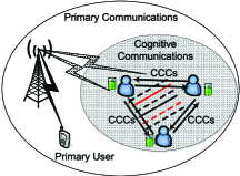
The focus on the previous sections are from a single SU’s perspective, where the proposed AOEECC-EXP3++ is an uncoordinated algorithm without cooperation with other SUs. It is well known that exploiting the cooperative behaviors among multiple SUs, such as cooperative spectrum sensing [4] and spectrum sharing [3], are effective approaches to improve the communication performance and EE of SUs. This section focuses on the accelerated learning by cooperative learning among multiple SUs. As we have noticed, considering information sharing among multi-users in MAB setting is recently a novel research direction, and we have seen initial results for stochastic MAB in [34]. Thus, our work can be regarded as the first one for both adversarial and stochastic MABs.

The cooperative learning can use Common Control Channels (CCCs) [3] to sharing information as illustrated in Fig. 2. Intuitively, when multiple SUs sening/probing multiple strategies simultaneously and exchange this information among them, this would offer more information for decision making, which results in faster learning and smaller regret value. At each timeslot $n$, suppose there are $L_{n}$ SUs cooperatively perform the $\epsilon$-SPA who wish to explore a total of $L_{n}$ strategeis over the total of the $N$ ($1\leq{L_{n}}\leq N$) and picks a subsect ${\mathcal{O}_{n}}\subseteq\left\{{1,...,N}\right\}$ of $L_{n}$ strategies to probe and observe the channel losses and power strategies to get the EE. Note that the channels losses that belong to the un-sensed and un-probed set of strategies $\mathcal{P}\setminus\mathcal{O}_{n}$ are still unrevealed. Accordingly, we have the probed and observed set of channels $\tilde{\mathcal{O}}_{n}$ with the simple property $f\in\tilde{\mathcal{O}}_{n},\forall f\in i\in\mathcal{O}_{n}$. The proposed algorithm 2 based on Algorithm 1 that considers fully information sharing among $L_{n}$ SUs such that for a single SU $u$. The probability $\bm{\varrho}_{n,u}=\bm{\varrho}_{n}=(\varrho_{n}(\mathbf{1}),...,\varrho_{n}(\mathbf{N}))$ of each observed strategy is

$\displaystyle\!\!{\varrho_{n}}(i)={{p_{n}(i)}}+\left({1-{{p_{n}(i)}}}\right)\frac{{{M_{n}}-1}}{{{N}-1}},\ if\ i\ \in\mathcal{O}_{n},$ (25)

where a mixture of the new exploration probability $(L_{n}-1)/(N-1)$ is introduced and $p_{n}(i)$ is defined in (5). Similarly, the channel probability ${\tilde{\varrho}}_{n}=({\tilde{\varrho}}_{n}({1})...,{\tilde{\varrho}}_{n}({n}))$ is computed as

$\displaystyle\!\!{\tilde{\varrho}_{n}}(f)={\rho_{n}}(f)+\left({1-{\rho_{n}}(f)}\right)\frac{{{m_{n}}-1}}{{{K}-1}},\ if\ f\ \in\mathcal{\tilde{O}}_{n}.$ (26)

Here, we have a channel-level new mixing exploration probability $(m_{n}-1)/(n-1)$ and ${\rho_{n}}(f)$ is defined in (6). The probing rate $m_{n}$ denotes the number of simultaneous sensed/probed/accessed non-overlapping channels among all SUs at timeslot $n$. Assume the weights of channels measured by different probes of different SUs within the same time slot also satisfy the assumption in Section II-A. The design of (25) and (26) is well thought out and the proof of all results in this section are non-trivial tasks in our unified framework.

Algorithm 2 Cooperative AOEECC-EXP3++: Multi-user Multi-channel $\epsilon$-SPA scheme
  Input: $M_{1},M_{2},...,$, such that $M_{n}\in\mathcal{P}$. Set $\beta_{n},{\varepsilon_{n}}\left(f\right),{\xi_{n}}\left(f\right)$ at in Alg. 1. $\forall i\in\mathcal{P},\tilde{L}_{0}(i)=0$ and $\forall f\in E,\tilde{\ell}_{0}(f)=0$.
  for  timeslot $n=1,2,...$ do
     1: Choose one SPA strategy $H_{n}$ according to $\rho_{n}$ (5). Get advice $\pi_{n}^{H_{n}}$ as the selected strategy. Sample $M_{n}-1$ additional strategies uniformly over $N$. Denote the set of sampled strategies by $\mathcal{O}_{n}$, where $H_{n}\in\mathcal{O}_{n}$ and $|\mathcal{O}_{n}|=M_{n}$. Let $\mathds{1}_{n}^{h}=\mathds{1}_{\{h\in\mathcal{O}_{n}\}}$.
     2: Update the probabilities $\varrho_{n}(i)$ according to (25). The loss of the observed strategy is
$\displaystyle{\tilde{\psi}_{n}}(i)=\frac{{{{\ell}_{n}}(i)+\lambda_{n-1}{\textsf{P}}_{n-1}(i)}}{\varrho_{n}(i)}\mathds{1}_{n}^{h},\forall i\in{\mathcal{O}_{n}}.$ (27)
     3: Compute the probability of choosing each channel ${{\tilde{\rho}}_{n}}(f)$ that belongs to $i$ according to (6).
     4: let $\mathds{1}(f)_{n}=\mathds{1}(f)_{f\in h\in\mathcal{O}_{n}}$. Update the channel probabilities $\tilde{\varrho}_{n}(f)$ according to (26). The loss of the observed channel is
$\displaystyle{\tilde{\psi}_{n}}(f)=\frac{{{{\ell}_{n}}(f)+\lambda_{n-1}{\textsf{P}}_{n-1}(f)}}{{\tilde{\varrho}_{n}}(f)}\mathds{1}(f)_{n},\forall{f}\in{\tilde{\mathcal{O}}_{n}}.$ (28)
     5: Updates all weights ${w_{n}}\left(f\right),{{\bar{w}}_{n}}\left(i\right),W_{n}$, Lagrangian multiplier and channel access probability $\epsilon$ as in Algorithm 1.
  end for

VI-A The Performance Results of $\epsilon$-SPA with $\epsilon=1$

If $m_{n}$ is a constant or lower bounded by $m$, we have the following results. Define ${{{\hat{G}}_{n}}}(\epsilon)$ as the expected average EEs that can be achieved by the $\epsilon$-SPA scheme over $n$ rounds. The Theorem 16, Theorem 17, Theorem 18, Theorem 19, Theorem 20 and Theorem 21 bound the regret of EE, $\mathop{\max}\nolimits_{i\in{S_{r}}}\mathbb{E}_{i\sim{\textbf{p}_{n}}}\{{{G_{n,i}}}\}-\mathbb{E}[{{{\hat{G}}_{n}}(1)}]$ when set $\epsilon=1$. From these results, we see a rate of $m$ in accelerating of learning performance.

Theorem 16. Under the oblivious attack with same setting of Theorem 1, the regret of the AOEECC-EXP3++ algorithm in the cooperative learning with probing rate $m$ satisfies

$\displaystyle\begin{array}[]{l}\textup{Regret}_{n}={R(n)}_{\textbf{p}_{n}^{\textup{T}}\textsf{P}}\mathop{\leq}O(4\sqrt{n\frac{K}{m}\ln K})\\ \textup{Violation}_{n}=\mathbb{E}{[{\sum\nolimits_{t=1}^{n}{\textbf{p}_{t}^{\textup{T}}\tilde{\textsf{P}}_{t}-\textsf{P}_{o}}}]_{+}}\leq O(n^{\frac{3}{4}}).\end{array}$

Theorem 17. Under the $\theta$-memory-bounded adaptive attack with same setting of Theorem 3, the regret of the AOEECC-EXP3++ algorithm in the cooperative learning with probing rate $m$ satisfies

$\displaystyle\begin{array}[]{l}\textup{Regret}_{n}={R(n)}_{\textbf{p}_{n}^{\textup{T}}\textsf{P}}\leq O((\theta+1){(4{k}\sqrt{\frac{K}{m}\ln K})^{\frac{2}{3}}}{n^{\frac{2}{3}}}).\\ \textup{Violation}_{n}=\mathbb{E}{[{\sum\nolimits_{t=1}^{n}{\textbf{p}_{t}^{\textup{T}}\tilde{\textsf{P}}_{t}-\textsf{P}_{o}}}]_{+}}\leq O(n^{\frac{3}{4}}).\end{array}$

Considering the practical implementation in the stochastic regime by estimating the gap as (V-B1), then we have

Theorem 18. With all other parameters hold as in Theorem 4, the regret of the AOEECC-EXP3++ algorithm with ${\xi_{n}}(f)=\frac{{c{{\left({\ln n}\right)}^{2}}}}{{mt{{\hat{\Delta}}_{n-1}}{{(f)}^{2}}}}$ and $\delta_{n}=2\frac{k}{m}\sqrt{\frac{{K\ln K}}{n}}$ in the cooperative learning with probing rate $m$, in the stochastic regime satisfies

$\displaystyle\begin{array}[]{l}\textup{Regret}_{n}={R(n)}_{\textbf{p}_{n}^{\textup{T}}\textsf{P}}\mathop{\leq}O(\frac{kK}{m}\frac{{c\ln{{(n)}^{3}}}}{{\Delta_{f}}})\\ \textup{Violation}_{n}=\mathbb{E}{[{\sum\nolimits_{t=1}^{n}{\textbf{p}_{t}^{\textup{T}}\tilde{\textsf{P}}_{t}-\textsf{P}_{o}}}]_{+}}\leq O(n^{\frac{3}{4}}).\end{array}$

Theorem 19. With all other parameters hold as in Theorem 9, the regret of the AOEECC-EXP3++ algorithm with ${\xi_{n}}(f)=\frac{{c{{\left({\ln n}\right)}^{2}}}}{{mt{{\hat{\Delta}}_{n-1}}{{(f)}^{2}}}}$ and $\delta_{n}=2\frac{k}{m}\sqrt{\frac{{K\ln K}}{n}}$ under oblivious jamming attack in the cooperative learning with probing rate $m$, in the mixed stochastic and adversarial regime satisfies

$\displaystyle\begin{array}[]{l}\textup{Regret}_{n}={R(n)}_{\textbf{p}_{n}^{\textup{T}}\textsf{P}}\mathop{\leq}O(\frac{K(k-k_{j})}{m}\frac{{c\ln{{(n)}^{3}}}}{{\Delta_{f}}})\\ \hskip 91.04872pt+O(\frac{4k_{j}}{m}\sqrt{tK\ln K})\\ \textup{Violation}_{n}=\mathbb{E}{[{\sum\nolimits_{t=1}^{n}{\textbf{p}_{t}^{\textup{T}}\tilde{\textsf{P}}_{t}-\textsf{P}_{o}}}]_{+}}\leq O(n^{\frac{3}{4}}).\end{array}$

Theorem 20. With all other parameters hold as in Theorem 11, the regret of the AOEECC-EXP3++ algorithm with ${\xi_{n}}(f)=\frac{{c{{\left({\ln n}\right)}^{2}}}}{{mt{{\hat{\Delta}}_{n-1}}{{(f)}^{2}}}}$ and $\delta_{n}=2\frac{k}{m}\sqrt{\frac{{K\ln K}}{n}}$ in the cooperative learning with probing rate $m$, in the mixed stochastic and adversarial regime satisfies

$\displaystyle\begin{array}[]{l}\textup{Regret}_{n}={R(n)}_{\textbf{p}_{n}^{\textup{T}}\textsf{P}}\mathop{\leq}O(\frac{K(k-k_{j})}{m}\frac{{c\ln{{(n)}^{3}}}}{{\Delta_{f}}})\\ \hskip 62.59596pt+O((\theta+1)\frac{k_{j}}{m}{(4{k}\sqrt{K\ln K})^{\frac{2}{3}}}{n^{\frac{2}{3}}})\\ \textup{Violation}_{n}=\mathbb{E}{[{\sum\nolimits_{t=1}^{n}{\textbf{p}_{t}^{\textup{T}}\tilde{\textsf{P}}_{t}-\textsf{P}_{o}}}]_{+}}\leq O(n^{\frac{3}{4}}).\end{array}$

Theorem 21. With all other parameters hold as in Theorem 13, the regret of the AOEECC-EXP3++ algorithm in the cooperative learning with probing rate $m$ in the contaminated stochastic regime satisfies

$\displaystyle\begin{array}[]{l}\textup{Regret}_{n}={R(n)}_{\textbf{p}_{n}^{\textup{T}}\textsf{P}}\mathop{\leq}{O({\frac{{Kk\ln{{(n)}^{3}}}}{{m(1-2\zeta)\Delta_{f}}}})}+Kn_{3}^{*}\\ \textup{Violation}_{n}=\mathbb{E}{[{\sum\nolimits_{t=1}^{n}{\textbf{p}_{t}^{\textup{T}}\tilde{\textsf{P}}_{t}-\textsf{P}_{o}}}]_{+}}\leq O(n^{\frac{3}{4}}).\end{array}$

VI-B $\epsilon$-SPA and Cooperative Sensing/Probing Issues

Due to space limit, we do not plan to present the least EE performance guarantees in the cooperative learning scenarios for $\epsilon$-SPA with general $\epsilon$. Obviously, it is simply a division of factor $m$ in the regret bound parts as in the related Theorem 2, Theorem 4, Theorem 6, Theorem 8, Theorem 10, Theorem 12 and Theorem 14.

In addition, cooperative sensing are necessary to be adopted, where the cooperative sensing gain will improve the sensing/probing performance. The formula by considering energy detector with cooperative sensing can be found in many existing works, such as in [4]. Hence, the analysis of cooperative $\epsilon$-SPA-scheme of the AOEECC-EXP3++ on the issues of 1) Impact of sensing time and 2) Impact of probing time and others can follow the same line as in Section V.E.

VI-C Distributed Protocols with Multiple Users

While the cooperative learning scheme offers the optimal learning performance, the design of decentralized protocol without using a CCC is challenging issue [34]. As presented in Section III-Section V, the energy detector cannot differentiate spectrum usage of PUs and SUs, the opinion of channel qualities of each SU is also affected by other SUs. Notice that the $\epsilon$-SPA scheme of the AOEECC-EXP3++ developed previously are applicable for all SUs, where their observation of the best multi-channel access strategies are the same, if each of these channels has the same mean across the players.

For fully distributed solutions, we already have proposed solution as shown in Section III-Section V to let each SU run the $\epsilon$-SPA scheme based on their own observation. However, this will come to the situation that all the users will access the same set of channels that result in low efficiency. This could be resolved by applying an approach similar to the TDFS scheme [36] by introducing round-robin schemes among SUs. We leave the details on this point in future works.

VII Proofs of Regrets in Different Regimes

We prove the theorems of the performance results from the previous section in the order they were presented.

Lemma 1. (Dual Inequality) Let ${f_{t}}(\lambda)=\frac{\delta_{t}}{2}{\lambda^{2}}+\lambda(\textbf{p}_{t-1}^{\textup{T}}\tilde{\textsf{P}}_{t-1}-\textsf{P}_{o}),{\lambda_{t}}={[({\lambda_{t-1}}-\eta_{t-1}\sqrt{\gamma_{t-1}}\nabla{f_{t-1}}({\lambda_{t-1}}))]_{+}}$ and $\lambda_{1}=0$. Assuming $\eta_{n}>0$, we have

$\displaystyle\sum\limits_{t=1}^{n}\!{\left({\lambda_{t}\!-\!{\lambda}}\right)}(\textsf{P}_{o}-\textbf{p}_{t}^{\textup{T}}\tilde{\textsf{P}}_{t})\!+\!\!\frac{\delta_{n}}{2}\sum\limits_{t=1}^{n}\!{\left({\lambda_{t}^{2}\!-\!{\lambda^{2}}}\right)}\!\leq\!\frac{1}{{{\eta\sqrt{\gamma_{n}}}}}{{\lambda}^{2}}\!$
$\displaystyle\hskip 89.91081pt+\sum\limits_{t=1}^{n}\sqrt{\gamma_{t}}{\eta_{t}}+\sum\limits_{t=1}^{n}\frac{{{\eta_{t}}}}{2}{(\textbf{p}_{t}^{\textup{T}}\tilde{\textsf{P}}_{t})^{2}}\!.$ (35)
Proof:

First, we note that

$\displaystyle\begin{array}[]{l}{\lambda_{t}}={[({\lambda_{t-1}}-{\eta_{t-1}}\sqrt{\gamma_{t-1}}\nabla{f_{t-1}}({\lambda_{t-1}}))]_{+}}\\ \quad\ ={[(1-\delta_{t-1}{\eta_{t-1}\sqrt{\gamma_{t-1}}}){\lambda_{t-1}}\!+\!{\eta_{t-1}\sqrt{\gamma_{t-1}}}(\textsf{P}_{o}\!\!-\!\!\textbf{p}_{t-1}^{\textup{T}}\tilde{\textsf{P}}_{t-1})]_{+}}\\ \quad\ \leq{[(1-\delta_{t-1}{\eta_{t-1}\sqrt{\gamma_{t-1}}}){\lambda_{t-1}}\!+\!{\eta_{t-1}\sqrt{\gamma_{t-1}}}{\textsf{P}_{0}}]_{+}}\end{array}$

By induction on $\lambda_{t}$, we can obtain ${\lambda_{t}}\leq\frac{{{\textsf{P}_{0}}}}{\delta_{t}}$. Applying the standard analysis of online gradient descent [41] yields

$\displaystyle\begin{array}[]{l}{|{{\lambda_{t}}\!-\!\lambda}|^{2}}\!\\ ={|{{\Pi_{+}}[({\lambda_{t-1}}\!-\!{\eta_{t-1}}\sqrt{\gamma_{t-1}}(\delta_{t-1}{\lambda_{t-1}}+\textsf{P}_{o}\!-\!\textbf{p}_{t-1}^{\textup{T}}\tilde{\textsf{P}}_{t-1}))]\!-\!\lambda}|^{2}}\\ \leq{|{{\lambda_{t-1}}-\lambda}|^{2}}+{\eta_{t-1}}^{2}\gamma_{t-1}{|{\nabla{f_{t-1}}({\lambda_{t-1}})}|^{2}}\\ \quad-2({\lambda_{t-1}}-\lambda)({{\eta_{t-1}}\sqrt{\gamma_{t-1}}\nabla{f_{t-1}}({\lambda_{t-1}})})\\ \leq{|{{\lambda_{t-1}}-\lambda}|^{2}}+{\eta_{t-1}}^{2}\gamma_{t-1}{|{\nabla{f_{t-1}}({\lambda_{t-1}})}|^{2}}\\ \quad+2{\eta_{t-1}}\sqrt{\gamma_{t-1}}({{f_{t-1}}(\lambda)-{f_{t-1}}({\lambda_{t-1}})})\end{array}$

Then, rearrange terms, we get,

$\displaystyle\begin{array}[]{l}\!\!\!{f_{t-1}}({\lambda_{t-1}})\!-\!{f_{t-1}}(\lambda)\leq\frac{1}{{2{\eta_{t-1}}\sqrt{\gamma_{t-1}}}}({\left|{\lambda\!-\!{\lambda_{t-1}}}\right|^{2}}\!-\!{\left|{\lambda\!-\!{\lambda_{t-1}}}\right|^{2}})\\ \quad\quad\quad\quad\quad\quad\quad\quad\quad+\frac{{\sqrt{\gamma_{t-1}}{\eta_{t-1}}}}{2}{\left|{\nabla{f_{t-1}}({\lambda_{t-1}})}\right|^{2}}\\ \hskip 85.35826pt\leq\frac{1}{{2\sqrt{\gamma_{t-1}}{\eta_{t-1}}}}({\left|{\lambda\!-\!{\lambda_{t-1}}}\right|^{2}}\!-\!{\left|{\lambda\!-\!{\lambda_{t-1}}}\right|^{2}})\\ \quad\quad\quad\quad\quad\quad\quad\quad\quad+\frac{{{\sqrt{\gamma_{t-1}}\eta_{t-1}}}}{2}{(\textbf{p}_{t-1}^{\textup{T}}\tilde{\textsf{P}}_{t-1})^{2}}+{\eta_{t-1}}.\end{array}$

Note that $\eta_{t}$ varies with $t$. For the first term leading factor in the r.h.s of the above inequality, use the trick by letting $\eta_{n}=\eta_{t}$ as indicated in [20] (page 25), e.g. if $\eta_{t}=\frac{1}{{\sqrt{t}}}$, we have $\sum\nolimits_{t=1}^{n}{\frac{1}{{\sqrt{t}}}}\leq\smallint_{0}^{n}\frac{1}{{\sqrt{t}}}dt=2\sqrt{n}$, a factor of $2$ gap between $\eta_{n}$ and $\eta_{t}$. Thus, substitute $\eta_{t}$ by $\eta_{n}/2$ and expanding the terms on l.h.s and taking the sum over $t$, we obtain the inequality. ∎

VII-A The Adversarial Regime

The proof of Theorem 1 borrows some of the analysis of EXP3 of the loss model in [20]. However, the introduction of the new mixing exploration parameter and the truth of channel dependency as a special type of combinatorial MAB problem in the loss model makes the proof a non-trivial task, and we prove it for the first time.

Proof of Theorem 1.

Proof:

Note first that the following equalities can be easily verified: ${\mathbb{E}_{i\sim{\textbf{p}_{n}}}}{\tilde{\ell}_{n}}(i)={\ell_{n}}({I_{n}}),{\mathbb{E}_{{\tilde{\ell}_{n}}\sim{\textbf{p}_{n}}}}{\ell_{n}}(i)={\ell_{n}}(i),{\mathbb{E}_{i\sim{\textbf{p}_{n}}}}{\tilde{\ell}_{n}}{(i)^{2}}=\frac{{{\ell_{n}}{{({I_{n}})}^{2}}}}{{{p_{n}}({I_{n}})}}$ and ${\mathbb{E}_{{I_{n}}\sim{\textbf{p}_{n}}}}\frac{1}{{{p_{n}}({I_{n}})}}=N$.

Let $\tilde{\Phi}_{n}(i)={{\tilde{\ell}}_{n}}(i)+\lambda_{n}{{\tilde{\textsf{P}}}_{n}}(i)$. The regret with respect to $\tilde{\Phi}_{n}(i)$ , $R_{\tilde{\Phi}_{n}(i)}(n)$, is

$\displaystyle R_{\tilde{\Phi}_{n}(i)}(n)=\mathbb{E}_{n}\left[\sum\limits_{t=1}^{n}{{\mathbb{E}_{i\sim{\textbf{p}_{t}}}}\tilde{\Phi}_{n}(i)}-\sum\limits_{t=1}^{n}{{\mathbb{E}_{{I_{t}}\sim{\textbf{p}_{t}}}}\tilde{\Phi}_{n}(i)}\right].$

The key step here is to consider the expectation of the cumulative losses ${\tilde{\ell}_{n}}(i)$ in the sense of distribution $i\sim{\textbf{p}_{n}}$. For all strategies, we have the distribution vector $\textbf{q}_{n}=(q_{n}(1),...,q_{n}(N))$ with ${q_{n}}(i)=\frac{{{w_{n-1}}\left(i\right)}}{{{W_{n-1}}}}$ and for all the channels, we have vector $\textbf{q}_{n,f}=(q_{n,f}(1),...,q_{n,f}(K))$ with ${q_{n,f}}(f^{\prime})=\frac{{\sum\nolimits_{i:f\in i}{{w_{n-1}}\left(i\right)}}}{{{W_{n-1}}}}$. Let ${\varepsilon_{n}}(i)=\sum\nolimits_{f\in i}{{\varepsilon_{n}}(f)}$. However, because of the mixing terms of $p_{n}$, we need to introduce a few more notations. Let $\textbf{u }=({\underbrace{\sum\nolimits_{f\in 1}{{\varepsilon_{n}}(f)},...,\sum\nolimits_{f\in i}{{\varepsilon_{n}}(f)},...,\sum\nolimits_{f\in|\mathcal{C}|}{{\varepsilon_{n}}(f)}}_{i\in\mathcal{C}},\underbrace{0,...,0}_{i\notin\mathcal{C}}})$ be the distribution over all the strategies. Let ${\textbf{q}_{n}}=\frac{{{\textbf{p}_{n}}-\textbf{u}}}{{1-\sum\nolimits_{f}{{\varepsilon_{n}}(f)}}}$ be the distribution induced by AOEECC-EXP3++ at the time $n$ without mixing. Then we have:

$\displaystyle\!\!\begin{array}[]{l}{\mathbb{E}_{i\sim{\textbf{p}_{t}}}}{\tilde{\Phi}_{t}}(i)=({1-\sum\nolimits_{f}{{\varepsilon_{t}}(f)}}){\mathbb{E}_{i\sim{\textbf{q}_{t}}}}{\tilde{\Phi}_{t}}(i)+{\varepsilon_{t}}(i){\mathbb{E}_{i\sim\textbf{u}}}{\tilde{\Phi}_{t}}(i)\\ \quad\quad\quad\quad\ \ =({1-\sum\nolimits_{f}{{\varepsilon_{t}}(f)}})(\frac{1}{{{\eta_{t}}}}\ln{\mathbb{E}_{i\sim{\textbf{q}_{t}}}}\exp(-{\eta_{t}}({\tilde{\Phi}_{t}}(i)\\ \quad\quad\quad\quad\quad\ -{\mathbb{E}_{j\sim{\textbf{q}_{t}}}}{\tilde{\Phi}_{t}}(j))))\\ \quad\quad\quad\quad\quad\ -\frac{({1-\sum\nolimits_{f}{{\varepsilon_{t}}(f)}})}{{{\eta_{t}}}}\ln{\mathbb{E}_{i\sim{\textbf{q}_{t}}}}\exp(-{\eta_{t}}{\tilde{\Phi}_{t}}(i)))\\ \quad\quad\quad\quad\quad\ +{\mathbb{E}_{i\sim\textbf{u}}}{\tilde{\Phi}_{t}}(i).\end{array}$

In the second step, we use the inequalities $lnx\leq x-1$ and $exp(-x)-1+x\leq x^{2}/2$, for all $x\geq 0$, to obtain:

$\displaystyle\begin{array}[]{l}\ln{\mathbb{E}_{i\sim{\textbf{q}_{t}}}}\exp(-{\eta_{t}}({\tilde{\Phi}_{t}}(i)-{\mathbb{E}_{j\sim{\textbf{q}_{t}}}}{\tilde{\Phi}_{t}}(j)))\\ \quad\quad\quad=\ln{\mathbb{E}_{i\sim{\textbf{q}_{t}}}}\exp(-{\eta_{t}}{\tilde{\Phi}_{t}}(i))+{\eta_{t}}{\mathbb{E}_{j\sim{\textbf{q}_{t}}}}{\tilde{\Phi}_{t}}(j)\\ \quad\quad\quad\leq{\mathbb{E}_{i\sim{\textbf{q}_{t}}}}({\exp(-{\eta_{t}}{\tilde{\Phi}_{t}}(i))-1+{\eta_{t}}{\tilde{\Phi}_{t}}(j)})\\ \quad\quad\quad\mathop{\leq}\limits^{(a)}{\mathbb{E}_{i\sim{\textbf{q}_{t}}}}\frac{{\eta_{t}^{2}{\tilde{\Phi}_{t}}{{(i)}^{2}}}}{2}\mathop{\leq}\limits^{(b)}{\eta_{t}^{2}\mathbb{E}_{i\sim{\textbf{q}_{t}}}}{{{\tilde{\ell}_{t}}{{(i)}^{2}}}}+\lambda_{t}^{2}\eta_{t}^{2}{\mathbb{E}_{i\sim{\textbf{q}_{t}}}}{{{{\tilde{\textsf{P}}}_{n}}(i)}^{2}},\end{array}$

where we used $\frac{{{q_{n}}(i)}}{{{p_{n}}(i)}}\leq\frac{1}{{1-\sum\nolimits_{f}{{\varepsilon_{t}}(f)}}}$ in the above inequality $(a)$ and the fact ${(x+y)^{2}}\leq 2{x^{2}}+2{y^{2}}$ in the above inequality $(b)$. Moreover, take expectations over all random strategies of losses ${{\tilde{\ell}}_{t}}{(i)^{2}}$, we have

$\displaystyle\begin{array}[]{l}{\mathbb{E}_{n}}\left[{\mathbb{E}_{i\sim{\textbf{q}_{t}}}}{{\tilde{\ell}}_{t}}{(i)^{2}}\right]={\mathbb{E}_{n}}\left[\sum\limits_{i=1}^{N}{{{q}_{t}}(i){{\tilde{\ell}}_{t}}{{(i)}^{2}}}\right]\\ ={\mathbb{E}_{n}}\!\!\left[\sum\limits_{i=1}^{N}{{{q}_{t}}(i){{(\sum\limits_{f\in i}{{{\tilde{\ell}}_{t}}(f)})}^{2}}}\right]\!=\!{\mathbb{E}_{n}}\!\!\left[\sum\limits_{i=1}^{N}{{{q}_{t}}(i){k}\!\!\sum\limits_{f\in i}{{{\tilde{\ell}}_{t}}{{(f)}^{2}}}}\right]\\ =\!{\mathbb{E}_{n}}k\left[\!\sum\limits_{f=1}^{K}{{{\tilde{\ell}}_{t}}{{(f)}^{2}}}\!\!\!\!\sum\limits_{i\in{S_{r}}:f\in i}\!\!\!{{{q}_{t}}(i)}\right]\!=\!{k}{\mathbb{E}_{n}}\!\!\left[\!\sum\limits_{f^{\prime}=1}^{K}\!{{{\tilde{\ell}}_{t}}{{(f^{\prime})}^{2}}{q_{t,f}}(f^{\prime})}\right]\\ \end{array}$
$\displaystyle\begin{array}[]{l}={k}{\mathbb{E}_{n}}\left[{\sum\limits_{f^{\prime}=1}^{K}{{{\left({\frac{{{\ell_{n}}(f^{\prime})}}{{{\rho_{n}}(f^{\prime})}}{\mathds{1}_{n}}(f^{\prime})}\right)}^{2}}}{q_{t,f}}(f^{\prime})}\right]\\ \leq{k}{\mathbb{E}_{n}}\left[{\sum\limits_{f^{\prime}=1}^{K}{\frac{{{q_{t,f}}(f^{\prime})}}{{{\rho_{n}}{{(f^{\prime})}^{2}}}}{\mathds{1}_{n}}(f^{\prime})}}\right]={k}\sum\limits_{f^{\prime}=1}^{K}{\frac{{{q_{t,f}}(f^{\prime})}}{{{\rho_{n}}(f^{\prime})}}}\\ ={k}\sum\limits_{f^{\prime}=1}^{K}{\frac{{{q_{t,f}}(f^{\prime})}}{{\left({1-\sum\nolimits_{f}{{\varepsilon_{n}}(f)}}\right){q_{t,f}}(f^{\prime})+{\sum\nolimits_{f\in i}{{\varepsilon_{n}}(f)}}\left|{\left\{{i\in\mathcal{C}:f\in i}\right\}}\right|}}}\leq 2kK,\end{array}$

where the last inequality follows the fact that $({1-\sum\nolimits_{f}{{\varepsilon_{n}}(f)}})\geq\frac{1}{2}$ by the definition of ${{\varepsilon_{n}}(f)}$. Similarly,

$\displaystyle\begin{array}[]{l}{\mathbb{E}_{n}}\left[{\mathbb{E}_{i\sim{\textbf{q}_{t}}}}{{{{\tilde{\textsf{P}}}_{n}}(i)}^{2}}\right]\leq 2kK,\end{array}$

In the third step, note that ${{\tilde{L}}_{0}}(i)=0$. Let ${\Upsilon_{n}}(\eta)=\frac{1}{\eta}\ln\frac{1}{N}\sum\nolimits_{i=1}^{N}{\exp(-\eta{{\tilde{L}}_{n}}(i))}$ and ${\Upsilon_{0}}(\eta)=0$. The second term in (VIII-A) can be bounded by using the same technique in [20] (page 26-28). Let us substitute inequality (VII-A) into (VIII-A), and then substitute (VIII-A) into equation (VIII-A) and sum over $n$. Use the fact that the sum of expectation on $u$ and $\textbf{q}_{t}$ with respect to ${{{\tilde{\Phi}}_{t}}(j)}$ is less than ${\mathbb{E}_{{I_{t}}\sim{\textbf{p}_{t}}}}{{{\tilde{\Phi}}_{t}}(j)}$. Take expectation over all random strategies of losses up to time $n$, we obtain

$\displaystyle\begin{array}[]{l}{\mathbb{E}_{n}}\left[\sum\limits_{t=1}^{n}{\mathbb{E}_{i\sim{\textbf{p}_{t}}}}{{\tilde{\Phi}}_{t}}(i)\right]\leq 2kK\!\sum\limits_{t=1}^{n}\eta_{t}+2kK\!\sum\limits_{t=1}^{n}\eta_{t}\lambda_{t}^{2}+\frac{{\ln N}}{\eta_{n}}\\ \hskip 8.5359pt+{\mathbb{E}_{n}}\left[\sum\limits_{t=1}^{n}{\mathbb{E}_{{I_{t}}\sim{\textbf{p}_{t}}}}{{{\tilde{\Phi}}_{t}}(j)}\right]+{\mathbb{E}_{n}}\left[\sum\limits_{t=1}^{n-1}({{\Upsilon_{t}}({\eta_{t+1}})-{\Upsilon_{t}}({\eta_{t}}))})\right]\!.\end{array}$

The last term in the r.h.s of the inequality is less than or equals to zero as indicated in [20]. Then, we get

$\displaystyle R_{\tilde{\Phi}_{n}(i)}(n)=\mathbb{E}_{n}\left[\sum\limits_{t=1}^{n}{{\mathbb{E}_{i\sim{\textbf{p}_{t}}}}\tilde{\Phi}_{n}(i)}-\sum\limits_{t=1}^{n}{{\mathbb{E}_{{I_{t}}\sim{\textbf{p}_{t}}}}\tilde{\Phi}_{n}(i)}\right]$
$\displaystyle\hskip 39.83368pt\leq 2kK\!\sum\limits_{t=1}^{n}\eta_{t}+\frac{{\ln N}}{\eta_{n}}+2kK\!\sum\limits_{t=1}^{n}\eta_{t}\lambda_{t}^{2}$
$\displaystyle\hskip 19.91684pt\mathop{\leq}\limits^{(a)}2kK\!\sum\limits_{t=1}^{n}\eta_{t}+k\frac{{\ln K}}{\eta_{n}}+2kK\!\sum\limits_{t=1}^{n}\eta_{t}\lambda_{t}^{2}.$ (45)

Note that, the inequality $(a)$ is due to the fact that $N\leq K^{k}$.

Combine (35) and (45) gives that

$\displaystyle\begin{array}[]{l}\mathbb{E}\left[{\sum\limits_{t=1}^{n}{{\textbf{p}^{T}_{t}}{\ell_{t}}(i)-{\textbf{p}^{T}_{t}}{\ell_{t}}({I_{t}})}}\right]+\\ \hskip 68.28644pt\mathbb{E}\left[{\sum\limits_{t=1}^{n}{\lambda(\textbf{p}_{t}^{\textup{T}}\tilde{\textsf{P}}_{t}-\textsf{P}_{o})-\left({\frac{{\delta_{n}n}}{2}+\frac{1}{\eta\sqrt{\gamma_{t}}}}\right){\lambda^{2}}}}\right]\\ \mathop{\leq}\limits^{(a)}2kK\sum\limits_{t=1}^{n}{{\eta_{t}}}+k\frac{{\ln K}}{{{\eta_{n}}}}+\sum\limits_{t=1}^{n}{\eta_{t}\sqrt{\gamma_{t}}}+\left({kK\eta_{n}-\frac{\delta_{n}}{2}}\right)\sum\limits_{t=1}^{n}{\lambda_{t}^{2}}\\ \hskip 93.89418pt+\mathbb{E}\left[{\sum\limits_{t=1}^{n}{{\lambda_{t}}(\textbf{p}_{t}^{\textup{T}}\tilde{\textsf{P}}_{t}-\textsf{P}_{o})}}\right].\end{array}$

For the above inequality $(a)$, we use the trick by letting $\eta_{n}=\eta_{t}$ indicated in [16] (page 25) again to extract the $\eta_{t}$ from the sum of $\lambda_{t}^{2}$ over $n$ and the inequality in (VIII-A). Let ${kK\eta_{n}\leq\frac{\delta_{n}}{2}}$ by setting properly the values such that $\eta_{n}=O(\delta_{n})$ (shown in the next). Thus, the last two terms in the r.h.s of the above inequality is non-positive. By taking maximization over $\lambda$, we have

$\displaystyle\begin{array}[]{l}\!\!\mathbb{E}\!\left[{\mathop{\max}\limits_{\textbf{p}_{t}^{\textup{T}}\tilde{\textsf{P}}_{t}\leq\textsf{P}_{o}}\sum\limits_{t=1}^{n}{{\textbf{p}^{T}_{t}}{\ell_{t}}(i)-{\textbf{p}^{T}_{t}}{\ell_{t}}({I_{t}})}}\right]\!+\!\mathbb{E}\!\left[{\frac{{\left[{\sum\limits_{t=1}^{n}{(\textbf{p}_{t}^{\textup{T}}\tilde{\textsf{P}}_{t}-\textsf{P}_{o})}}\right]_{+}^{2}}}{{2\left({\delta n/2+{1\mathord{\left/{\vphantom{1\eta}}\right.\kern-1.2pt}\eta}}\right)}}}\right]\\ \hskip 93.89418pt\mathop{\leq}\limits^{(a)}2kK\sum\limits_{t=1}^{n}{{\eta_{t}}}+k\frac{{\ln K}}{{{\eta_{n}}}}+\sum\limits_{t=1}^{n}{\eta_{t}\sqrt{\gamma_{t}}}.\end{array}$

Note that our algorithm exhibit a bound in the structure like $\textup{Regret}_{n}+\frac{{\textup{Violation}_{n}^{2}}}{{O({n^{1-\alpha}})}}\leq{n^{1-\beta}}$. We can derive a regret bound and the violation of the long-term power budget constraint as

$\displaystyle\begin{array}[]{l}\textup{Regret}_{n}\leq O({n^{1-\beta}})\\ \textup{Violation}_{n}\leq\sqrt{O(\left[{n+{n^{1-\beta}}}\right]{n^{1-\alpha}})},\end{array}$

where the last bound follows the naive fact $-\textup{Regret}_{n}\leq O(n)$. In practice, we this bound is coarse, and we can us the accumulated variance to obtain better violation bound.

Then, according to (VII-A), we obtain

$\displaystyle\begin{array}[]{l}\mathbb{E}\left[{\mathop{\max}\limits_{\textbf{p}_{t}^{\textup{T}}\tilde{\textsf{P}}_{t}\leq\textsf{P}_{o}}\sum\limits_{t=1}^{n}{{\textbf{p}^{T}_{t}}{\ell_{t}}(i)-{\textbf{p}^{T}_{t}}{\ell_{t}}({I_{t}})}}\right]\mathop{\leq}\limits 4kKn{\eta_{n}}+k\frac{{\ln K}}{{{\eta_{n}}}}\\ \hskip 110.96556pt+\sum\limits_{t=1}^{n}{\eta_{t}\sqrt{\gamma_{t}}}\mathop{\leq}\limits 4k\sqrt{nK\ln K}\\ \mathbb{E}{\left[{\sum\limits_{t=1}^{n}{\textbf{p}_{t}^{\textup{T}}\tilde{\textsf{P}}_{t}-\textsf{P}_{o}}}\right]_{+}}\!\leq\!\sqrt{\!\left({n+4k\sqrt{nK\ln K}}\right)\left({\delta_{n}n+{2\mathord{\left/{\vphantom{1\eta}}\right.\kern-1.2pt}\eta_{n}}}\right)}.\end{array}$

Let ${\eta_{n}}={\beta_{n}}=\sqrt{\frac{{\ln K}}{{4Kn}}}=O\left({{n^{-1/2}}}\right),{1\mathord{\left/{\vphantom{1\eta_{n}}}\right.\kern-1.2pt}\eta}=O\left({{n^{1/2}}}\right)$. Because $\gamma_{n}=\tilde{O}(\frac{ln(n)}{n})$, the term $\sum\nolimits_{t=1}^{n}{\eta_{t}\sqrt{\gamma_{t}}}=\tilde{O}(ln(n))$. Thus, it can be omitted when compared to the first two terms in the r.h.s of (VIII-A). Moreover, in this setting, we set $\delta_{n}=2k\sqrt{\frac{{K\ln K}}{n}}$, such that ${2kK\eta_{n}\leq\frac{\delta_{n}}{2}}$. Then, $\delta_{n}n=O\left({{n^{1/2}}}\right)$. We proof the theorem. ∎

Proof of Theorem 3.

Proof:

To defend against the $\theta$-memory-bounded adaptive adversary, we need to adopt the idea of the mini-batch protocol proposed in [29]. We define a new algorithm by wrapping AOEECC-EXP3++ with a mini-batching loop [31]. We specify a batch size $\tau$ and name the new algorithm AOEECC-EXP3++τ. The idea is to group the overall timeslots $1,...,n$ into consecutive and disjoint mini-batches of size $\tau$. It can be viewed that one signal mini-batch as a round (timeslot) and use the average loss suffered during that mini-batch to feed the original AOEECC-EXP3++. Note that our new algorithm does not need to know $m$, which only appears as a constant as shown in Theorem 2. So our new AOEECC-EXP3++τ algorithm still runs in an adaptive way without any prior about the environment. If we set the batch $\tau={(4{k}\sqrt{K\ln K})^{-\frac{1}{3}}}{n^{{}^{\frac{1}{3}}}}$ in Theorem 2 of [29], we can get the regret upper bound in our Theorem 2. ∎

VII-B The Stochastic Regime

Our proofs are based on the following form of Bernstein’s inequality with minor improvement as shown in [35].

Lemma 2. (Bernstein’s inequality for martingales). Let $X_{1},...,X_{m}$ be martingale difference sequence with respect to filtration $\mathcal{F}=(\mathcal{F}_{i})_{1\leq k\leq m}$ and let $Y_{k}=\sum\nolimits_{j=1}^{k}{{X_{j}}}$ be the associated martingale. Assume that there exist positive numbers $\nu$ and $c$, such that $X_{j}\leq c$ for all $j$ with probability $1$ and $\sum\nolimits_{k=1}^{m}{\mathbb{E}\left[{{{\left({{X_{k}}}\right)}^{2}}|{\mathcal{F}_{k-1}}}\right]}\leq\nu$ with probability 1.

$\displaystyle\mathbb{P}[{Y_{m}}>\sqrt{2\nu b}+\frac{{cb}}{3}]\leq{e^{-b}}.$

Lemma 3. Let $\left\{{{{\underline{\varepsilon}}_{n}}(f)}\right\}_{n=1}^{\infty}$ be non-increasing deterministic sequences, such that ${{\underline{\varepsilon}}_{n}}(f)\leq{{\varepsilon}_{n}}(f)$ with probability $1$ and ${{\underline{\varepsilon}}_{n}}(f)\leq{{\varepsilon}_{n}}(f^{*})$ for all $n$ and $f$. Define $\nu_{n}(f)=\sum\nolimits_{t=1}^{n}\frac{1}{{{k\underline{\varepsilon}}_{t}}(f)}$, and define the event $\mathcal{E}^{f}_{n}$

$\displaystyle{n\Delta(f)-({{{\tilde{L}}_{n}}(f^{*})-{{\tilde{L}}_{n}}({f})})}$
$\displaystyle\hskip 36.98866pt\leq{\sqrt{2({\nu_{n}}(f)+{\nu_{n}}({f^{*}})){b_{n}}}+\frac{{{(1/k+0.25)}{b_{n}}}}{{3k{\underline{\varepsilon}_{n}}({f^{*}})}}}\hskip 8.5359pt(\mathcal{E}^{f}_{n}).$

Then for any positive sequence $b_{1},b_{2},...,$ and any $n^{*}\geq 2$ the number of times channel $f$ is played by AOEECC-EXP3++ up to round $n$ is bounded as:

$\displaystyle\begin{array}[]{l}\mathbb{E}[{N_{n}}(f)]\leq\left({{n^{*}}-1}\right)+\sum\limits_{t={n^{*}}}^{n}{{e^{-{b_{t}}}}}+k\sum\limits_{t={n^{*}}}^{n}{{\varepsilon_{t}}(f){\mathds{1}_{\{E_{n}^{f}\}}}}\\ \hskip 36.98866pt+\sum\limits_{t={n^{*}}}^{n}{{e^{-{\eta_{t}}{h_{t}}(f)}}}e^{-\eta_{t}\lambda_{t}({{\tilde{\Gamma}}_{t}}(f^{*})\!-\!{{\tilde{\Gamma}}_{t}}(f))},\end{array}$

where

$\displaystyle\begin{array}[]{l}{h_{n}}(f)=n\Delta(f)-\sqrt{2n{b_{n}}\left({\frac{1}{{{k}{{\underline{\varepsilon}}_{n}}(f)}}+\frac{1}{{{k}{{\underline{\varepsilon}}_{n}}({f^{*}})}}}\right)}-\frac{{(\frac{1}{4}+\frac{1}{k}){b_{n}}}}{{3{{\underline{\varepsilon}}_{n}}({f^{*}})}}.\end{array}$
Proof:

Note that the elements of the martingale difference sequence $\{{\Delta(f)-({{\tilde{\ell}}_{n}}(f)-{{\tilde{\ell}}_{n}}({f^{*}}))}\}_{n=1}^{\infty}$ by $\max\{\Delta(f)+{{\tilde{\ell}}_{n}}({f^{*}})\}={\frac{1}{{{k}{{\underline{\varepsilon}}_{n}}({f^{*}})}}}+1$. Since ${{{\underline{\varepsilon}}_{n}}({f^{*}})}\leq{{{\varepsilon}_{n}}({f^{*}})}\leq 1/(2K)\leq 1/4$, we can simplify the upper bound by using ${\frac{1}{{{{k\underline{\varepsilon}}_{n}}({f^{*}})}}}+1\leq\frac{{(\frac{1}{4}+\frac{1}{k})}}{{{{\underline{\varepsilon}}_{n}}({f^{*}})}}$.

We further note that

$$\begin{array}[]{l}\sum\limits_{t=1}^{n}{{\mathbb{E}_{t}}\left[{{(\Delta(f)-({{\tilde{\ell}}_{t}}(f)-{{\tilde{\ell}}_{t}}({f^{*}})))}^{2}}\right]}\\ \hskip 31.2982pt\leq\sum\limits_{t=1}^{n}{{\mathbb{E}_{t}}\left[{{({{\tilde{\ell}}_{t}}(f)-{{\tilde{\ell}}_{t}}({f^{*}}))}^{2}}\right]}\\ \hskip 31.2982pt=\sum\limits_{t=1}^{n}{\left({{\mathbb{E}_{t}}\left[({{\tilde{\ell}}_{t}}{{(f)}^{2}}\right]+{E_{t}}\left[({{\tilde{\ell}}_{t}}{{({f^{*}})}^{2}}\right]}\right)}\\ \hskip 31.2982pt\leq\sum\limits_{t=1}^{n}\left({\frac{1}{{{\rho_{t}}(f)}}+\frac{1}{{{\rho_{t}}({f^{*}})}}}\right)\\ \hskip 31.2982pt\mathop{\leq}\limits^{(a)}\sum\limits_{t=1}^{n}{\left({\frac{1}{{k{\varepsilon_{t}}(f)}}+\frac{1}{{k{\varepsilon_{t}}({f^{*}})}}}\right)}\\ \hskip 31.2982pt\leq\sum\limits_{t=1}^{n}{\left({\frac{1}{{k{{\underline{\varepsilon}}_{t}}(f)}}+\frac{1}{{k{{\underline{\varepsilon}}_{t}}({f^{*}})}}}\right)}={\nu_{t}}(f)+{\nu_{t}}({f^{*}})\end{array}$$

with probability $1$. The above inequality (a) is due to the fact that $q_{n}(f)\geq\sum\nolimits_{f\in i}{{\varepsilon_{n}}(f)}\left|{\left\{{i\in\mathcal{C}:f\in i}\right\}}\right|$. Since each $f$ only belongs to one of the covering strategies $i\in\mathcal{C}$, $\left|{\left\{{i\in\mathcal{C}:f\in i}\right\}}\right|$ equals to 1 at time slot $n$ if channel $f$ is selected. Thus, $q_{n}(f)\geq\sum\nolimits_{f\in i}{{\varepsilon_{n}}(f)}=k{\varepsilon_{n}}(f)$.

Let $\mathcal{\bar{E}}_{n}^{f}$ denote the complementary of event $\mathcal{E}_{n}^{f}$. Then by the Bernstein’s inequality $\mathbb{P}[\mathcal{\bar{E}}_{n}^{f}]\leq e^{-b_{n}}$. The number of times the channel $f$ is selected up to round $n$ is bounded as:

$\displaystyle\begin{array}[]{l}\mathbb{E}[{N_{n}}(f)]=\sum\limits_{t=1}^{n}{\mathbb{P}[A_{t}=f]}\\ \hskip 40.00006pt=\sum\limits_{t=1}^{n}{\mathbb{P}[A_{t}=f|\mathcal{E}_{t-1}^{f}]P[\mathcal{E}_{t-1}^{f}]}\\ \hskip 50.00008pt+\mathbb{P}[A_{t}=f|\overline{\mathcal{E}_{t-1}^{f}}]P[\overline{\mathcal{E}_{t-1}^{f}}]\\ \hskip 40.00006pt\leq\sum\limits_{t=1}^{n}{\mathbb{P}[A_{t}=f|\mathcal{E}_{t-1}^{f}]}{\mathds{1}_{\{\mathcal{E}_{t-1}^{f}\}}}+\mathbb{P}[\overline{\mathcal{E}_{t-1}^{S}}]\\ \hskip 40.00006pt\leq\sum\limits_{t=1}^{n}{\mathbb{P}[A_{t}=f|\mathcal{E}_{t-1}^{f}]}{\mathds{1}_{\{\mathcal{E}_{t-1}^{f}\}}}+{e^{-{b_{t-1}}}}.\end{array}$

We further upper bound ${\mathbb{P}[A_{t}=f|\mathcal{E}_{t-1}^{f}]}{\mathds{1}_{\{\mathcal{E}_{t-1}^{f}\}}}$ as follows:

$$\begin{array}[]{l}\mathbb{P}{[A_{t}=f|{\cal\mathcal{E}}_{t-1}^{f}]}{\mathds{1}_{\{{\cal\mathcal{E}}_{t-1}^{f}\}}}\end{array}$$
$$\hskip 8.00003pt\begin{array}[]{l}={\rho_{t}}(f){\mathds{1}_{\{{\cal\mathcal{E}}_{t-1}^{f}\}}}\\ \leq({q_{t}}(f)+k{\varepsilon_{t}}(f)){\mathds{1}_{\{{\cal\mathcal{E}}_{t-1}^{f}\}}}\\ =({k\varepsilon_{t}}(f)+\frac{{\sum\nolimits_{i:f\in i}{{w_{t-1}}\left(i\right)}}}{{{W_{t-1}}}}){\mathds{1}_{\{{\cal\mathcal{E}}_{t-1}^{f}\}}}\\ =({k\varepsilon_{t}}(f)+\frac{{\sum\nolimits_{i:f\in i}{{e^{-{\eta_{t}}{{\tilde{\Psi}}_{t}}(i)}}}}}{{\sum\nolimits_{i=1}^{N}{{e^{-{\eta_{t}}{{\tilde{\Psi}}_{t}}(i)}}}}}){\mathds{1}_{\{{\cal\mathcal{E}}_{t-1}^{f}\}}}\\ \mathop{\leq}\limits^{(a)}({k\varepsilon_{t}}(f)+{e^{-{\eta_{t}}\left({{{\tilde{\Psi}}_{t}}(i)-{{\tilde{\Psi}}_{t}}({i^{*}})}\right)}}){\mathds{1}_{\{{\cal\mathcal{E}}_{t-1}^{f}\}}}\\ \mathop{\leq}\limits^{(b)}({k\varepsilon_{t}}(f)+{e^{-{\eta_{t}}\left({{\tilde{\Psi}_{t}}(f)-{{\tilde{\Psi}}_{t}}({f^{*}})}\right)}}){\mathds{1}_{\{{\cal\mathcal{E}}_{t-1}^{f}\}}}\\ =({k\varepsilon_{t}}(f)\\ \hskip 1.00006pt+{e^{-{\eta_{t}}\left({{\tilde{L}}}_{t}(f)-{{\tilde{L}}}_{t}(f^{*})+\lambda_{t}({{\tilde{\Gamma}}_{t}}(f^{*})-{{\tilde{\Gamma}}_{t}}(f))\right)}}){\mathds{1}_{\{{\cal\mathcal{E}}_{t-1}^{f}\}}}\\ \end{array}$$
$$\begin{array}[]{l}\mathop{\leq}\limits^{(c)}k{\varepsilon_{t}}(f){\mathds{1}_{\{{\cal\mathcal{E}}_{t-1}^{f}\}}}\!+\!{e^{-{\eta_{t}}{h_{t}}(f)}}e^{-\eta_{t}\lambda_{t}({{\tilde{\Gamma}}_{t}}(f^{*})\!-\!{{\tilde{\Gamma}}_{t}}(f))}\end{array}$$

The above inequality (a) is due to the fact that channel $f$ only belongs to one selected strategy $i$ at $t$, inequality (b) is because the cumulative regret of each strategy is great than the cumulative regret of each channel that belongs to the strategy, inequality (c) is due to the fact that ${{{\underline{\varepsilon}}_{t}}(f)}$ is a non-increasing sequence ${\upsilon_{t}}(f)\leq\frac{t}{{{{k\underline{\varepsilon}}_{t}}(f)}}$. Substitution of this result back into the computation of $\mathbb{E}[{N_{n}}(f)]$ completes the proof. ∎

Proof of Theorem 5.

Proof:

The proof is based on Lemma 1 and Lemma 3. Combine (35) and (VII-B)

$\displaystyle\begin{array}[]{l}\mathbb{E}\left[{\sum\limits_{t=1}^{n}{{\textbf{p}_{t}^{T}}{\ell_{t}}(i)-{\textbf{p}_{t}^{T}}{\ell_{t}}({I_{t}})}}\right]+\\ \hskip 85.35826pt\mathbb{E}\left[{\sum\limits_{t=1}^{n}{\lambda(\textbf{p}_{t}^{\textup{T}}\tilde{\textsf{P}}_{t}-\textsf{P}_{o})-\left({\frac{{\delta n}}{2}+\frac{1}{\eta}}\right){\lambda^{2}}}}\right]\\ \hskip 8.5359pt\mathop{\leq}\sum\limits_{f=1}^{K}\mathbb{E}[{N_{n}}(f)]\Delta(f)+\sum\limits_{t=1}^{n}{\eta_{t}\sqrt{\gamma_{t}}}\\ \hskip 99.58464pt\!-\!{\frac{\delta}{2}}\sum\limits_{t=1}^{n}{\lambda_{t}^{2}}+\!\mathbb{E}\left[{\sum\limits_{t=1}^{n}{{\lambda_{t}}(\textbf{p}_{t}^{\textup{T}}\tilde{\textsf{P}}_{t}-\textsf{P}_{o})}}\right]\!.\end{array}$

Obviously, the last two terms in the r.h.s of the above inequality is negative. By taking maximization over $\lambda$, we have

$\displaystyle\begin{array}[]{l}\!\!\!\!\!\mathbb{E}\left[{\mathop{\max}\limits_{\textbf{p}_{t}^{\textup{T}}\tilde{\textsf{P}}_{t}\leq\textsf{P}_{o}}\sum\limits_{t=1}^{n}{{\textbf{p}_{t}^{T}}{\ell_{t}}(i)-{\textbf{p}_{t}^{T}}{\ell_{t}}({I_{t}})}}\right]\!\!+\!\mathbb{E}\!\left[\!{\frac{{\left[{\sum\limits_{t=1}^{n}{(\textbf{p}_{t}^{\textup{T}}\tilde{\textsf{P}}_{t}-\textsf{P}_{o})}}\right]_{+}^{2}}}{{2\left({\delta n/2+{1\mathord{\left/{\vphantom{1\eta}}\right.\kern-1.2pt}\eta}}\right)}}}\right]\\ \hskip 91.04872pt\mathop{\leq}\sum\limits_{f=1}^{K}\mathbb{E}[{N_{n}}(f)]\Delta(f)+\sum\limits_{t=1}^{n}{\eta_{t}\sqrt{\gamma_{t}}}.\end{array}$

Set $b_{n}=ln(n\Delta(f)^{2})$, ${{{\underline{\varepsilon}}_{n}}(f)}={{{\varepsilon}_{n}}(f)}$ and ${{{\varepsilon}_{n}}(f)}=\frac{{{b_{n}}}}{{n\Delta{{\left(f\right)}^{2}}}}$. Thus, $\gamma_{n}=\sum\nolimits_{f=1}^{K}{{\varepsilon_{n}}\left(f\right)}=\sum\nolimits_{f=1}^{K}\frac{{\ln(n\Delta{{\left(f\right)}^{2}})}}{{n\Delta{{\left(f\right)}^{2}}}}=O(\frac{{\ln(n)}}{n})$. For any $c\geq 18$ and any $n\geq n^{*}$, where $n^{*}$ is the minimal integer for which ${n^{*}}\geq\frac{{4{c^{2}}K\ln{{({n^{*}}\Delta{{(f)}^{2}})}^{2}}}}{{\Delta{{(f)}^{4}}\ln(K)}}$, we have

$$\begin{array}[]{l}{h_{n}}(f)=n\Delta(f)-\sqrt{2n{b_{n}}\left({\frac{1}{{k{\varepsilon_{n}}(f)}}+\frac{1}{{k{\varepsilon_{n}}({f^{*}})}}}\right)}-\frac{{\left({\frac{1}{4}+\frac{1}{k}}\right){b_{n}}}}{{3{\varepsilon_{n}}({f^{*}})}}\\ \hskip 24.29996pt\geq n\Delta(f)-2\sqrt{\frac{{n{b_{n}}}}{{k{\varepsilon_{n}}(f)}}}-\frac{{\left({\frac{1}{4}+\frac{1}{k}}\right){b_{n}}}}{{3{\varepsilon_{n}}(f)}}\\ \hskip 24.29996pt=n\Delta(f)(1-\frac{2}{{\sqrt{kc}}}-\frac{{\left({\frac{1}{4}+\frac{1}{k}}\right)}}{{3c}})\\ \hskip 24.29996pt\mathop{\geq}\limits^{(a)}n\Delta(f)(1-\frac{2}{{\sqrt{c}}}-\frac{{1.25}}{{3c}})\geq\frac{1}{2}n\Delta(f).\end{array}$$

The above inequality (a) is due to the fact that $(1-\frac{2}{{\sqrt{kc}}}-\frac{{\left({\frac{1}{4}+\frac{1}{k}}\right)}}{{3c}}$ is an increasing function with respect to $k(k\geq 1)$. The transmission power is quasi-concave to the reward such that the accumulated power allocation strategy have $(-h_{t}(f)+\lambda_{t}({{\tilde{\Gamma}}_{t}}(f)-{{\tilde{\Gamma}}_{t}}(f^{*})))\leq 0$, and by substitution of the lower bound on $h_{n}(f)$ into Lemma 3. Thus, we have

$\displaystyle\begin{array}[]{l}\!\!\!\mathbb{E}[{N_{n}}(f)]\!\leq\!\frac{{\ln(n)}}{{\Delta{{(f)}^{2}}}}\!+\!k\frac{{c\ln{{(n)}^{2}}}}{{\Delta{{(f)}^{2}}}}\!+\!{n^{*}}\!+\!\sum\limits_{t=1}^{n}\!\!\left(\!{{e^{-\frac{{\Delta(f)}}{4}\sqrt{\frac{{(t-1)ln(K)}}{K}}}}}\!\right)\\ \hskip 35.00005pt\leq k\frac{{c\ln{{(n)}^{2}}}}{{\Delta{{(f)}^{2}}}}+\frac{{\ln(n)}}{{\Delta{{(f)}^{2}}}}+{n^{*}}+O(\frac{{{K}}}{{\Delta{{(f)}^{2}}}}),\end{array}$

where we used Lemma 3 to bound the sum of the exponents in the first two terms. In addition, please note that $n^{*}$ is of the order $O(\frac{{kK}}{{\Delta{{(f)}^{4}}\ln(K)}})$. The last term is bounded by Lemma 10 in [35].

The (VII-B) bounds the first item in the r.h.s of (VII-B). For the second term, since $\eta_{n}\!\!=\!\!\frac{1}{2}\sqrt{\frac{{\ln K}}{{nK}}}$, $\sum\nolimits_{t=1}^{n}{\eta_{t}\sqrt{\gamma_{t}}}=O(\sqrt{ln(n)})$. That indicates

$\displaystyle\begin{array}[]{l}\!\!\!\!\!\mathbb{E}\!\left[{\mathop{\max}\limits_{\textbf{p}_{t}^{\textup{T}}\tilde{\textsf{P}}_{t}\leq\textsf{P}_{o}}\sum\limits_{t=1}^{n}{{\textbf{p}_{t}^{T}}{\ell_{t}}(i)-{\textbf{p}_{t}^{T}}{\ell_{t}}({I_{t}})}}\right]\!\!+\!\!\mathbb{E}\!\!\left[\!{\frac{{\left[{\sum\limits_{t=1}^{n}{(\textbf{p}_{t}^{\textup{T}}\tilde{\textsf{P}}_{t}-\textsf{P}_{o})}}\right]_{+}^{2}}}{{\left({\delta n+\sqrt{\frac{{nK}}{{\ln K}}}}\right)}}}\right]\\ \mathop{\leq}k\frac{{c\ln{{(n)}^{2}}}}{{\Delta{{(f)}}}}+\frac{{\ln(n)}}{{\Delta{{(f)}}}}+O(\frac{{{K}}}{{\Delta{{(f)}}}})+{n^{*}}+O(\sqrt{ln(n)}).\end{array}$

Moreover, set $\delta=2k\sqrt{\frac{{K\ln K}}{n}}$, we have ${kK\eta\leq\frac{\delta}{2}}$ and ${{\delta n+\sqrt{\frac{{nK}}{{\ln K}}}}}\simeq\left({2k+1}\right)\sqrt{2Kn}=O(\sqrt{n})$. Then, we obtain

$\displaystyle\begin{array}[]{l}\mathbb{E}\left[{\mathop{\max}\limits_{\textbf{p}_{t}^{\textup{T}}\tilde{\textsf{P}}_{t}-\textsf{P}_{o}}\sum\limits_{t=1}^{n}{{\textbf{p}_{t}^{T}}{\ell_{t}}(i)-{\textbf{p}_{t}^{T}}{\ell_{t}}({I_{t}})}}\right]\mathop{\leq}O(k\frac{{c\ln{{(n)}^{2}}}}{{\Delta{{(f)}}}})\\ \mathbb{E}{\left[{\sum\limits_{t=1}^{n}{\textbf{p}_{t}^{\textup{T}}\tilde{\textsf{P}}_{t}-\textsf{P}_{o}}}\right]_{+}}\!\leq\!\sqrt{\!({n+k\frac{{c\ln{{(n)}^{2}}}}{{\Delta{{(f)}}}}}){({\delta n+\sqrt{\frac{{nK}}{{\ln K}}}})}}\\ \hskip 85.00012pt=O(n^{\frac{3}{4}}).\end{array}$

Thus, we proof the theorem. ∎

Proof of Theorem 7.

Proof:

The proof is based on the similar idea of Theorem 5, Lemma 1 and Lemma 3. Here, we just show the difference part. Note that by our definition ${{\hat{\Delta}}_{n}}(f)\leq 1$ and the sequence ${\underline{\varepsilon}_{n}}(f)={\underline{\varepsilon}_{n}}=\min\{\frac{1}{{2K}},{\beta_{n}},\frac{{c\ln{{(n)}^{2}}}}{n}\}$ satisfies the condition of Lemma 10. Note that when ${\beta_{n}}\geq\frac{{c\ln{{(n)}^{2}}}}{n}\}$, i.e., for $n$ large enough such that $n\geq\frac{{4{c^{2}}\ln{{(n)}^{4}}K}}{{\ln(K)}}$, we have ${\underline{\varepsilon}_{n}}=\frac{{c\ln{{(n)}^{2}}}}{n}$. Let $b_{n}=ln(n)$ and let $n^{*}$ be large enough, so that for all $n\geq n^{*}$ we have $n\geq\frac{{4{c^{2}}\ln{{(n)}^{4}}K}}{{\ln(K)}}$ and $n\geq e^{\frac{1}{\Delta(f)^{2}}}$. With these parameters and conditions on hand, we are going to bound the rest of the three terms in the bound on $\mathbb{E}[N_{n}(f)]$ in Lemma 10. The upper bound of $\sum\nolimits_{t={n^{*}}}^{n}{{e^{-{b_{t}}}}}$ is easy to obtain. For bounding $k\sum\nolimits_{t={n^{*}}}^{n}{{\varepsilon_{t}}(f){\mathds{1}_{\{\mathcal{E}_{t-1}^{f}\}}}}$, we note that $\mathcal{E}_{n}^{f}$ holds and we have

$$\begin{array}[]{l}{{\hat{\Delta}}_{n}}(f)\geq\frac{1}{n}(\mathop{\max}\limits_{k}({{\tilde{L}}_{n}}(k))-{{\tilde{L}}_{n}}(f))\geq\frac{1}{n}({{\tilde{L}}_{n}}({f^{*}})-{{\tilde{L}}_{n}}(f))\\ \hskip 24.29996pt\geq\frac{1}{n}{h_{n}}(f)=\frac{1}{n}\left({n\Delta(f)-2\sqrt{\frac{{n{b_{n}}}}{{k{{\underline{\varepsilon}}_{n}}}}}-\frac{{(\frac{1}{4}+\frac{1}{k}){b_{n}}}}{{3{{\underline{\varepsilon}}_{n}}}}}\right)\\ \hskip 24.29996pt=\frac{1}{n}\left({n\Delta(f)-\frac{{2n}}{{\sqrt{ck\ln(n)}}}-\frac{{(\frac{1}{4}+\frac{1}{k})n}}{{3c\ln(n)}}}\right)\\ \hskip 24.29996pt\mathop{\geq}\limits^{(a)}\frac{1}{n}\left({n\Delta(f)-\frac{{2n}}{{\sqrt{c\ln(n)}}}-\frac{{1.25n}}{{3c\ln(n)}}}\right)\\ \hskip 24.29996pt\mathop{\geq}\limits^{(b)}\Delta(f)\left({1-\frac{2}{{\sqrt{c}}}-\frac{{1.25}}{{3c}}}\right)\geq\frac{1}{2}\Delta(f),\end{array}$$

where the inequality (a) is due to the fact that $\frac{1}{n}(n\Delta(f)-\frac{2n}{\sqrt{ck\ln(n)}}-\frac{(\frac{1}{4}+\frac{1}{k})n}{3c\ln(n)})$ is an increasing function with respect to $k(k\geq 1)$ and the inequality (b) due to the fact that for $n\geq n^{*}$ we have $\sqrt{ln(n)}\geq 1/\Delta(f).$ Thus,

$${\varepsilon_{K}}(f){\mathds{1}_{\{\mathcal{E}_{K-1}^{f}\}}}\leq\frac{{c{{\left({\ln n}\right)}^{2}}}}{{n{{\hat{\Delta}}_{n}}{{(f)}^{2}}}}\leq\frac{{4{c^{2}}{{\left({\ln n}\right)}^{2}}}}{{n\Delta{{(f)}^{2}}}}$$

and $k\sum\nolimits_{t={n^{*}}}^{n}{{\varepsilon_{t}}(f){\mathds{1}_{\{\mathcal{E}_{K-1}^{f}\}}}}=O\left({\frac{{k\ln{{\left(n\right)}^{3}}}}{{\Delta{{(f)}^{2}}}}}\right)$. Finally, for the last term in Lemma 10, we have already get $h_{n}(f)\geq\frac{1}{2}\Delta(f)$ for $n\geq n^{*}$ as an intermediate step in the calculation of bound on ${{{\hat{\Delta}}_{n}}(f)}$. Therefore, the last term is bounded in a order of $O(\frac{{{K}}}{{\Delta{{(f)}^{2}}}})$. Use all these results together we obtain the results of the theorem. Note that the results holds for any $\eta_{n}\geq\beta_{n}$. ∎

VII-C Mixed Adversarial and Stochastic Regime

Proof of Theorem 9.

Proof:

The proof of the regret performance in the mixed adversarial and stochastic regime is simply a combination of the performance of the AOEECC-EXP3++${}^{\emph{AVG}}$ algorithm in adversarial and stochastic regimes. It is very straightforward from Theorem 1 and Theorem 7. ∎

Proof of Theorem 11.

Proof:

Similar as above, the proof is very straightforward from Theorem 3 and Theorem 7. ∎

VII-D Contaminated Stochastic Regime

Proof of Theorem 13.

Proof:

The key idea of proving the regret bound under moderately contaminated stochastic regime relies on how to estimate the performance loss by taking into account the contaminated pairs. The rest of the proof is based on the similar idea of Theorem 7, Lemma 1 and Lemma 3. Here, we just show the difference part. Let $\mathds{1}_{n,f}^{\star}$ denote the indicator functions of the occurrence of contamination at location $(n,f)$, i.e., $\mathds{1}_{n,f}^{\star}$ takes value $1$ if contamination occurs and 00 otherwise. Let $m_{n}(f)=\mathds{1}_{n,f}^{\star}\tilde{\ell}_{n}(f)+(1-\mathds{1}_{n,f}^{\star})\mu(f)$. If either base arm $f$ was contaminated on round $n$ then $m_{n}(f)$ is adversarially assigned a value of loss that is arbitrarily affected by some adversary, otherwise we use the expected loss. Let ${M_{n}}(f)=\sum\nolimits_{t=1}^{n}{{m_{n}}(f)}$ then $\left({{M_{n}}({f})-{M_{n}}(f^{*})}\right)-\left({{{\tilde{L}}_{n}}({f})-{{\tilde{L}}_{n}}(f^{*})}\right)$ is a martingale. After $\tau$ steps, for $n\geq\tau$,

$$\begin{array}[]{l}\left({{M_{n}}({f})-{M_{n}}(f^{*})}\right)\geq n\min\{\mathds{1}_{n,f}^{\star},\mathds{1}_{n,f^{*}}^{\star}\}({\tilde{\ell}_{n}}(f)-{\tilde{\ell}_{n}}({f^{*}}))\\ \hskip 60.00009pt+n\min\{1-\mathds{1}_{n,f}^{\star},1-\mathds{1}_{n,f^{*}}^{\star}\}(\mu({f})-\mu(f^{*}))\\ \hskip 36.0001pt\geq-\zeta n\Delta(f)+(n-\zeta n\Delta(f))\Delta(f)\geq(1-2\zeta){n\Delta(f)}.\end{array}$$

Define the event $\mathcal{Z}_{n}^{f}$:

$$(1-2\zeta)n\Delta(f)-\left({{{\tilde{L}}_{n}}({f})-{{\tilde{L}}_{n}}(f^{*})}\right)\leq 2\sqrt{{\nu_{n}}{b_{n}}}+\frac{{\left({\frac{1}{4}+\frac{1}{k}}\right){b_{n}}}}{{3{{\underline{\varepsilon}}_{n}}}},$$

where ${\underline{\varepsilon}}_{n}$ is defined in the proof of Theorem 2 and $\nu_{n}=\sum\nolimits_{t=1}^{n}{\frac{1}{{{{k\underline{\varepsilon}}_{n}}}}}$. Then by Bernstein’s inequality $\mathbb{P}[\mathcal{Z}_{n}^{f}]\leq e^{-b_{n}}$. The remanning proof is identical to the proof of Theorem 2.

For the regret performance in the moderately contaminated stochastic regime, according to our definition with the attacking strength $\zeta\in[0,1/4]$, we only need to replace $\Delta(f)$ by $\Delta(f)/2$ in Theorem 4. ∎

VIII Proof of Regret for Accelerated AOEECC Algorithm

We prove the theorems of the performance results in Section VI in the order they were presented.

VIII-A Accelerated Learning in Adversarial Regime

The proof the Theorem 16 requires the following Lemma from Lemma 7 [49]. We restate it for completeness.

Lemma 4. For any probability distribution $\omega$ on $\{1,...,K\}$ and any $m\in[K]$:

$\displaystyle\sum\limits_{f=1}^{n}{\frac{{\omega(f)(K-1)}}{{\omega(f)(K-m)+m-1}}\leq\frac{K}{m}}.$

Proof of Theorem 16.

Proof:

With similar facts and notations as in the proof of Theorem 1, we have: Then we have:

$\displaystyle\!\!\begin{array}[]{l}{\mathbb{E}_{i\sim{\textbf{p}_{t}}}}{\tilde{\Phi}_{t}}(i)=({1-\sum\nolimits_{f}{{\varepsilon_{t}}(f)}}){\mathbb{E}_{i\sim{\textbf{q}_{t}}}}{\tilde{\Phi}_{t}}(i)+{\varepsilon_{t}}(i){\mathbb{E}_{i\sim\textbf{u}}}{\tilde{\Phi}_{t}}(i)\\ \quad\quad\quad\quad\ \ =({1-\sum\nolimits_{f}{{\varepsilon_{t}}(f)}})(\frac{1}{{{\eta_{t}}}}\ln{\mathbb{E}_{i\sim{\textbf{q}_{t}}}}\exp(-{\eta_{t}}({\tilde{\Phi}_{t}}(i)\\ \quad\quad\quad\quad\quad\ -{\mathbb{E}_{j\sim{\textbf{q}_{t}}}}{\tilde{\Phi}_{t}}(j))))\\ \quad\quad\quad\quad\quad\ -\frac{({1-\sum\nolimits_{f}{{\varepsilon_{t}}(f)}})}{{{\eta_{t}}}}\ln{\mathbb{E}_{i\sim{\textbf{q}_{t}}}}\exp(-{\eta_{t}}{\tilde{\Phi}_{t}}(i)))\\ \quad\quad\quad\quad\quad\ +{\mathbb{E}_{i\sim\textbf{u}}}{\tilde{\Phi}_{t}}(i).\end{array}$

In the second step, we use the inequalities $lnx\leq x-1$ and $exp(-x)-1+x\leq x^{2}/2$, for all $x\geq 0$, to obtain:

$\displaystyle\begin{array}[]{l}\ln{\mathbb{E}_{i\sim{\textbf{q}_{t}}}}\exp(-{\eta_{t}}({\tilde{\Phi}_{t}}(i)-{\mathbb{E}_{j\sim{\textbf{q}_{t}}}}{\tilde{\Phi}_{t}}(j)))\\ \quad\quad\quad=\ln{\mathbb{E}_{i\sim{\textbf{q}_{t}}}}\exp(-{\eta_{t}}{\tilde{\Phi}_{t}}(i))+{\eta_{t}}{\mathbb{E}_{j\sim{\textbf{q}_{t}}}}{\tilde{\Phi}_{t}}(j)\\ \quad\quad\quad\leq{\mathbb{E}_{i\sim{\textbf{q}_{t}}}}({\exp(-{\eta_{t}}{\tilde{\Phi}_{t}}(i))-1+{\eta_{t}}{\tilde{\Phi}_{t}}(j)})\\ \quad\quad\quad\mathop{\leq}\limits^{(a)}{\mathbb{E}_{i\sim{\textbf{q}_{t}}}}\frac{{\eta_{t}^{2}{\tilde{\Phi}_{t}}{{(i)}^{2}}}}{2}\mathop{\leq}\limits^{(b)}{\eta_{t}^{2}\mathbb{E}_{i\sim{\textbf{q}_{t}}}}{{{\tilde{\ell}_{t}}{{(i)}^{2}}}}+\lambda_{t}^{2}\eta_{t}^{2}{\mathbb{E}_{i\sim{\textbf{q}_{t}}}}{{{{\tilde{\textsf{P}}}_{n}}(i)}^{2}},\end{array}$

Take expectations over all random strategies of losses ${{\tilde{\ell}}_{t}}{(i)^{2}}$, we have

$\displaystyle\begin{array}[]{l}\!\!\!{\mathbb{E}_{n}}\left[{\mathbb{E}_{i\sim{{q}_{t}}}}{{\tilde{\ell}}_{t}}{(i)^{2}}\right]={\mathbb{E}_{n}}\left[\sum\limits_{i=1}^{N}{{{q}_{t}}(i){{\tilde{\ell}}_{t}}{{(i)}^{2}}}\right]\\ \!\!\!\!={\mathbb{E}_{n}}\!\!\left[\sum\limits_{i=1}^{N}{{{q}_{t}}(i){{(\sum\limits_{f\in i}{{{\tilde{\ell}}_{t}}(f)})}^{2}}}\right]\leq{\mathbb{E}_{n}}\!\!\left[\sum\limits_{i=1}^{N}{{{q}_{t}}(i){k}\!\!\sum\limits_{f\in i}{{{\tilde{\ell}}_{t}}{{(f)}^{2}}}}\right]\\ \!\!\!\!=\!{\mathbb{E}_{n}}k\left[\!\sum\limits_{f=1}^{K}{{{\tilde{\ell}}_{t}}{{(f)}^{2}}}\!\!\!\!\sum\limits_{i\in{\mathcal{P}}:f\in i}\!\!\!{{{q}_{t}}(i)}\right]\!=\!{k}{\mathbb{E}_{n}}\!\!\left[\!\sum\limits_{f^{\prime}=1}^{K}\!{{{\tilde{\ell}}_{t}}{{(f^{\prime})}^{2}}{q_{t,f}}(f^{\prime})}\right]\\ \!\!\!\!={k}{\mathbb{E}_{n}}\left[{\sum\limits_{f^{\prime}=1}^{K}{{{\left({\frac{{{\ell_{t}}(f)}}{{{{{\tilde{\varrho}}_{t}}}(f)}}{\mathds{1}_{t}}(f)}\right)}^{2}}}{q_{t,f}}(f^{\prime})}\right]\\ \end{array}$
$\displaystyle\begin{array}[]{l}\!\!\!\!\leq{k}{\mathbb{E}_{n}}\left[{\sum\limits_{f=1}^{K}{\frac{{{q_{t,f}}(f)}}{{{{{\tilde{\varrho}}_{t}}}{{(f)}^{2}}}}{\mathds{1}_{t}}(f)}}\right]={k}\sum\limits_{f=1}^{K}{\frac{{q_{t,f}(f)}}{{{{{\tilde{\varrho}}_{t}}}(f)}}}\\ \!\!\!\!={k}\!\!\sum\limits_{f=1}^{K}\!\!{\frac{{q_{t-1,f}(f)}}{{{\rho_{t}}(f)+(1-{\rho_{t}}(f))\frac{{{m_{t}}-1}}{{{K}-1}}}}}\mathop{\leq}\limits^{(a)}{k}\!\!\sum\limits_{f=1}^{K}\!\!{\frac{{2\rho_{t}}(f)}{{{\rho_{n}}(f)+(1-{\rho_{t}}(f))\frac{{{m_{t}}-1}}{{{K}-1}}}}}\\ \mathop{\leq}\limits^{(b)}2k\frac{K}{m},\end{array}$

where the above inequality $(a)$ follows the fact that $({1-\sum\nolimits_{f}{{\varepsilon_{t}}(f)}})\geq\frac{1}{2}$ by the definition of ${{\varepsilon_{t}}(f)}$ and the equality (26) and the above inequality $(b)$ follows the Lemma 4. Similarly,

$\displaystyle\begin{array}[]{l}{\mathbb{E}_{n}}\left[{\mathbb{E}_{i\sim{\textbf{q}_{t}}}}{{{{\tilde{\textsf{P}}}_{n}}(i)}^{2}}\right]\leq 2k\frac{K}{m},\end{array}$

Note that ${\varphi_{t-1}}(f)=\sum\nolimits_{f\in i}{{\varepsilon_{n}}(f)}\left|{\left\{{i\in\mathcal{C}:f\in i}\right\}}\right|,\forall f\in[1,n]$ Take expectations over all random strategies of losses ${{\tilde{\ell}}_{t}}{(i)}$ with respective to distribution $u$, we have

$\displaystyle\begin{array}[]{l}{\mathbb{E}_{n}}\left[{\mathbb{E}_{i\sim{\varphi_{t}}}}{{\tilde{\ell}}_{t}}{(i)}\right]={\mathbb{E}_{n}}\left[\sum\limits_{i=1}^{N}{{\varphi_{t}}(i){{\tilde{\ell}}_{t}}{{(i)}}}\right]\\ ={\mathbb{E}_{n}}\!\!\left[\sum\limits_{i=1}^{N}{{\varphi_{t}}(i){{(\sum\limits_{f\in i}{{{\tilde{\ell}}_{t}}(f)})}}}\right]\leq{\mathbb{E}_{n}}\!\!\left[\sum\limits_{i=1}^{N}{{\varphi_{t}}(i)(\sum\limits_{f\in i}{{{\tilde{\ell}}_{t}}{{(f)})}}}\right]\\ =\!{\mathbb{E}_{n}}\left[\!\sum\limits_{f=1}^{K}{{{\tilde{\ell}}_{t}}{{(f)}}}\!\!\!\!\sum\limits_{i\in{\mathcal{P}}:f\in i}\!\!\!{{\varphi_{t}}(i)}\right]\!=\!{}{\mathbb{E}_{n}}\!\!\left[\!\sum\limits_{f^{\prime}=1}^{K}\!{{{\tilde{\ell}}_{t}}{{(f^{\prime})}}{\varphi_{t}}(f^{\prime})}\right]\\ \leq{k}{\mathbb{E}_{n}}\left[{\sum\limits_{f^{\prime}=1}^{K}{\frac{{\varphi_{t}}(f^{\prime})}{{{{{\tilde{\rho}}_{t}}}{{(f^{\prime})}}}}{\mathds{1}_{t}}(f^{\prime})}}\right]={k}\sum\limits_{f^{\prime}=1}^{K}{\frac{{\varphi_{t}}(f^{\prime})}{{{{{\tilde{\rho}}_{t}}}(f^{\prime})}}}\\ ={k}\sum\limits_{f^{\prime}=1}^{K}{\frac{{\varphi_{t}}(f^{\prime})}{{\tilde{\rho}_{t}}(f)+(1-{\tilde{\rho}_{t}}(f))\frac{{{m_{t}}-1}}{{{K}-1}}}}\\ \mathop{\leq}\limits^{(a)}{k}\sum\limits_{f^{\prime}=1}^{K}{\frac{{\tilde{\rho}_{t}}(f)}{{\tilde{\rho}_{t}}(f)+(1-{\tilde{\rho}_{t}}(f))\frac{{{m_{t}}-1}}{{{K}-1}}}}\mathop{\leq}\limits^{(b)}2k\frac{K}{m},\end{array}$

where the above inequality $(a)$ is due to the fact that ${\tilde{\rho}_{n}}(f)\geq{\varphi_{t-1}}(f)$ and the above inequality $(b)$ follows the Lemma 4.

In the third step, take expectation over all random strategies of losses up to time $n$, we obtain

$\displaystyle\begin{array}[]{l}{\mathbb{E}_{n}}\left[\sum\limits_{t=1}^{n}{\mathbb{E}_{i\sim{\textbf{p}_{t}}}}{{\tilde{\Phi}}_{t}}(i)\right]\leq\frac{2kK}{m}\!\sum\limits_{t=1}^{n}\eta_{t}+\frac{2kK}{m}\!\sum\limits_{t=1}^{n}\eta_{t}\lambda_{t}^{2}+\frac{{\ln N}}{\eta_{n}}\\ \hskip 8.5359pt+{\mathbb{E}_{n}}\left[\sum\limits_{t=1}^{n}{\mathbb{E}_{{I_{t}}\sim{\textbf{p}_{t}}}}{{{\tilde{\Phi}}_{t}}(j)}\right]+{\mathbb{E}_{n}}\left[\sum\limits_{t=1}^{n-1}({{\Upsilon_{t}}({\eta_{t+1}})-{\Upsilon_{t}}({\eta_{t}}))})\right]\!.\end{array}$

The last term in the r.h.s of the inequality is less than or equals to zero as indicated in [20]. Then, we get

$\displaystyle R_{\tilde{\Phi}_{n}(i)}(n)=\mathbb{E}_{n}\left[\sum\limits_{t=1}^{n}{{\mathbb{E}_{i\sim{\textbf{p}_{t}}}}\tilde{\Phi}_{n}(i)}-\sum\limits_{t=1}^{n}{{\mathbb{E}_{{I_{t}}\sim{\textbf{p}_{t}}}}\tilde{\Phi}_{n}(i)}\right]$
$\displaystyle\hskip 39.83368pt\leq\frac{2kK}{m}\!\sum\limits_{t=1}^{n}\eta_{t}+\frac{{\ln N}}{\eta_{n}}+\frac{2kK}{m}\!\sum\limits_{t=1}^{n}\eta_{t}\lambda_{t}^{2}$
$\displaystyle\hskip 19.91684pt\mathop{\leq}\limits^{(a)}\frac{2kK}{m}\!\sum\limits_{t=1}^{n}\eta_{t}+k\frac{{\ln K}}{\eta_{n}}+\frac{2kK}{m}\!\sum\limits_{t=1}^{n}\eta_{t}\lambda_{t}^{2}.$ (65)

Note that, the inequality $(a)$ is due to the fact that $N\leq K^{k}$.

Combine (35) and (45) gives that

$\displaystyle\begin{array}[]{l}\mathbb{E}\left[{\sum\limits_{t=1}^{n}{{\textbf{p}^{T}_{t}}{\ell_{t}}(i)-{\textbf{p}^{T}_{t}}{\ell_{t}}({I_{t}})}}\right]+\\ \hskip 68.28644pt\mathbb{E}\left[{\sum\limits_{t=1}^{n}{\lambda(\textbf{p}_{t}^{\textup{T}}\tilde{\textsf{P}}_{t}-\textsf{P}_{o})-\left({\frac{{\delta_{n}n}}{2}+\frac{1}{\eta\sqrt{\gamma_{t}}}}\right){\lambda^{2}}}}\right]\\ \mathop{\leq}\limits^{(a)}\frac{2kK}{m}\sum\limits_{t=1}^{n}{{\eta_{t}}}+k\frac{{\ln K}}{{{\eta_{n}}}}+\sum\limits_{t=1}^{n}{\eta_{t}\sqrt{\gamma_{t}}}+\left({\frac{kK}{m}\eta_{n}-\frac{\delta_{n}}{2}}\right)\sum\limits_{t=1}^{n}{\lambda_{t}^{2}}\\ \hskip 93.89418pt+\mathbb{E}\left[{\sum\limits_{t=1}^{n}{{\lambda_{t}}(\textbf{p}_{t}^{\textup{T}}\tilde{\textsf{P}}_{t}-\textsf{P}_{o})}}\right].\end{array}$

For the above inequality $(a)$, we use the trick by letting $\eta_{n}=\eta_{t}$ indicated in [16] (page 25) again to extract the $\eta_{t}$ from the sum of $\lambda_{t}^{2}$ over $n$ and the inequality in (VIII-A). Let ${kK\eta_{n}\leq\frac{m\delta_{n}}{2}}$ by setting properly the values such that $\eta_{n}=O(\delta_{n})$ (shown in the next). Thus, the last two terms in the r.h.s of the above inequality is non-positive. By taking maximization over $\lambda$, we have

$\displaystyle\begin{array}[]{l}\!\!\!\mathbb{E}\!\left[{\mathop{\max}\limits_{\textbf{p}_{t}^{\textup{T}}\tilde{\textsf{P}}_{t}\leq\textsf{P}_{o}}\sum\limits_{t=1}^{n}{{\textbf{p}^{T}_{t}}{\ell_{t}}(i)-{\textbf{p}^{T}_{t}}{\ell_{t}}({I_{t}})}}\right]\!\!+\!\mathbb{E}\!\!\left[{\frac{{\left[{\sum\limits_{t=1}^{n}{(\textbf{p}_{t}^{\textup{T}}\tilde{\textsf{P}}_{t}-\textsf{P}_{o})}}\right]_{+}^{2}}}{{2\left({\delta n/2+{1\mathord{\left/{\vphantom{1\eta}}\right.\kern-1.2pt}\eta}}\right)}}}\right]\\ \hskip 93.89418pt\mathop{\leq}\limits^{(a)}\frac{2kK}{m}\sum\limits_{t=1}^{n}{{\eta_{t}}}+k\frac{{\ln K}}{{{\eta_{n}}}}+\sum\limits_{t=1}^{n}{\eta_{t}\sqrt{\gamma_{t}}}.\end{array}$

Then, we obtain

$\displaystyle\begin{array}[]{l}\mathbb{E}\left[{\mathop{\max}\limits_{\textbf{p}_{t}^{\textup{T}}\tilde{\textsf{P}}_{t}\leq\textsf{P}_{o}}\sum\limits_{t=1}^{n}{{\textbf{p}^{T}_{t}}{\ell_{t}}(i)-{\textbf{p}^{T}_{t}}{\ell_{t}}({I_{t}})}}\right]\mathop{\leq}\limits\frac{4kK}{m}n{\eta_{n}}+k\frac{{\ln K}}{{{\eta_{n}}}}\\ \hskip 110.96556pt+\sum\limits_{t=1}^{n}{\eta_{t}\sqrt{\gamma_{t}}}\mathop{\leq}\limits 4k\sqrt{n\frac{K}{m}\ln K}\\ \mathbb{E}{\left[{\sum\limits_{t=1}^{n}{\textbf{p}_{t}^{\textup{T}}\tilde{\textsf{P}}_{t}-\textsf{P}_{o}}}\right]_{+}}\!\leq\!\sqrt{\!\left({n+4k\sqrt{nK\ln K}}\right)\left({\delta_{n}n+{2\mathord{\left/{\vphantom{1\eta}}\right.\kern-1.2pt}\eta_{n}}}\right)}.\end{array}$

Let ${\eta_{n}}={\beta_{n}}=\sqrt{\frac{{\ln K}}{{4Kn}}}=O\left({{n^{-1/2}}}\right),{1\mathord{\left/{\vphantom{1\eta_{n}}}\right.\kern-1.2pt}\eta}=O\left({{n^{1/2}}}\right)$. Because $\gamma_{n}=\tilde{O}(\frac{ln(n)}{n})$, the term $\sum\nolimits_{t=1}^{n}{\eta_{t}\sqrt{\gamma_{t}}}=\tilde{O}(ln(n))$. Thus, it can be omitted when compared to the first two terms in the r.h.s of (VIII-A). Moreover, in this setting, we set $\delta_{n}=2\frac{k}{m}\sqrt{\frac{{K\ln K}}{n}}$, such that ${2kK\eta_{n}\leq\frac{m\delta_{n}}{2}}$. Then, $\delta_{n}n=O\left({{n^{1/2}}}\right)$. This completes the proof. ∎

Proof of Theorem 17.

Proof:

The proof of Theorem 17 for adaptive adversary uses the same idea as in the proof of Theorem 2. Here, if we set the batch $\tau={(4{k}\sqrt{\frac{n}{m}\ln n})^{-\frac{1}{3}}}{n^{{}^{\frac{1}{3}}}}$ in Theorem 2 of [29], we can get the regret upper bound in our Theorem 17. ∎

VIII-B Cooperative Learning of AOEECC in Stochastic Regime

To obtain the tight regret performance for cooperative learning of AOEECC-EXP3++, we need to study and estimate the number of times each of channel is selected up to time $n$, i.f., $N_{n}(f)$. We summarize it in the following lemma.

Lemma 5. In the multipath probing case, let $\left\{{{{\underline{\varepsilon}}_{n}}(f)}\right\}_{n=1}^{\infty}$ be non-increasing deterministic sequences, such that ${{\underline{\varepsilon}}_{n}}(f)\leq{{\varepsilon}_{n}}(f)$ with probability $1$ and ${{\underline{\varepsilon}}_{n}}(f)\leq{{\varepsilon}_{n}}(f^{*})$ for all $n$ and $f$. Define $\nu_{n}(f)=\sum\nolimits_{t={1}}^{n}\frac{1}{{{k\underline{\varepsilon}}_{t}}(f)}$, and define the event $\Xi^{f}_{n}$

$\displaystyle{mt\Delta(f)-({{{\tilde{L}}_{n}}(f^{*})-{{\tilde{L}}_{n}}({f})})}$
$\displaystyle\hskip 8.5359pt\leq{\sqrt{2({\nu_{n}}(f)+{\nu_{n}}({f^{*}})){b_{n}}}+\frac{{{(1/k+0.25)}{b_{n}}}}{{3k{\underline{\varepsilon}_{n}}({f^{*}})}}}\hskip 8.5359pt(\Xi^{f}_{n}).$

Then for any positive sequence $b_{1},b_{2},...,$ and any $n^{*}\geq 2$ the number of times channel $f$ is played by AOEECC-EXP3++ up to round $n$ is bounded as:

$\displaystyle\begin{array}[]{l}\mathbb{E}[{N_{n}}(f)]\leq\left({{n^{*}}-1}\right)+\sum\limits_{t={n^{*}}}^{n}{{f^{-{b_{t}}}}}+k\sum\limits_{t={n^{*}}}^{n}{{\varepsilon_{t}}(f){\mathds{1}_{\{\Xi_{n}^{f}\}}}}\\ \hskip 45.52458pt+\sum\limits_{t={n^{*}}}^{n}{{f^{-{\eta_{t}}{\hslash_{t-1}}(f)}}}e^{-\eta_{t}\lambda_{t}({{\tilde{\Gamma}}_{t}}(f^{*})\!-\!{{\tilde{\Gamma}}_{t}}(f))},\end{array}$

where

$\displaystyle\begin{array}[]{l}{\hslash_{n}}(f)={mt}\Delta(f)-\sqrt{2{mt}{b_{n}}\left({\frac{1}{{{k}{{\underline{\varepsilon}}_{n}}(f)}}+\frac{1}{{{k}{{\underline{\varepsilon}}_{n}}({f^{*}})}}}\right)}-\frac{{(\frac{1}{4}+\frac{1}{k}){b_{n}}}}{{3{{\underline{\varepsilon}}_{n}}({f^{*}})}}.\end{array}$
Proof:

Note that AOEECC-EXP3++ probes $L_{n}$ strategies rather than $1$ strategy each timeslot $n$. Let $\#\left\{\cdot\right\}$ stands for the number of elements in the set $\left\{\cdot\right\}$. Hence,

$\displaystyle\begin{array}[]{l}\mathbb{E}[{N_{n}}(f)]=\mathbb{E}[\#\left\{{1\leq t\leq n:{A_{t}}=f,\mathcal{E}_{n}^{f}}\right\}+\\ \hskip 113.81102pt\#\left\{{1\leq t\leq n:{A_{t}}=f,\overline{\mathcal{E}_{n}^{f}}}\right\}],\end{array}$

where $A_{t}$ denotes the action of channel selection at timeslot $t$. By the following simple trick, we have

$\displaystyle\begin{array}[]{l}\!\!\!\!\!\!\!\!\mathbb{E}[{N_{n}}(f)]=\mathbb{E}[\#\left\{{1\leq t\leq n:{A_{t}}=f,\mathcal{E}_{n}^{f}}\right\}]+\\ \hskip 88.2037pt\mathbb{E}[\#\left\{{1\leq t\leq n:{A_{t}}=f,\overline{\mathcal{E}_{n}^{f}}}\right\}]]\\ \hskip 11.38092pt\leq\mathbb{E}[\sum\limits_{t=1}^{n}\mathds{1}_{\left\{{1\leq t\leq n:{A_{t}}=f}\right\}}\mathbb{P}[\#\{\mathcal{E}_{n}^{f}\}]]+\\ \hskip 88.2037pt\mathbb{E}[\sum\limits_{t=1}^{n}\mathds{1}_{\left\{{1\leq t\leq n:{A_{t}}=f}\right\}}\mathbb{P}[\#\{\overline{\mathcal{E}_{n}^{f}}\}]]\\ \hskip 11.38092pt\leq\mathbb{E}[\sum\limits_{t=1}^{n}\mathds{1}_{\left\{{1\leq t\leq n:{A_{t}}=f}\right\}}\mathbb{P}[\Xi_{mt}^{f}]]+\\ \hskip 88.2037pt\mathbb{E}[\sum\limits_{t=1}^{n}\mathds{1}_{\left\{{1\leq t\leq n:{A_{t}}=f}\right\}}\mathbb{P}[\Xi_{mt}^{f}]].\end{array}$

Note that the elements of the martingale difference sequence in the $\{{\Delta(f)-({{\tilde{\ell}}_{n}}(f)-{{\tilde{\ell}}_{n}}({f^{*}}))}\}_{n=1}^{\infty}$ by $\max\{\Delta(f)+{{\tilde{\ell}}_{n}}({f^{*}})\}={\frac{1}{{{k}{{\underline{\varepsilon}}_{n}}({f^{*}})}}}+1$. Since ${{{\underline{\varepsilon}}_{n}}({f^{*}})}\leq{{{\varepsilon}_{n}}({f^{*}})}\leq 1/(2n)\leq 1/4$, we can simplify the upper bound by using ${\frac{1}{{{{k\underline{\varepsilon}}_{n}}({f^{*}})}}}+1\leq\frac{{(\frac{1}{4}+\frac{1}{k})}}{{{{\underline{\varepsilon}}_{n}}({f^{*}})}}$.

We further note that

$$\begin{array}[]{l}{\mathbb{E}_{t}}\left\{\#\left\{\sum\limits_{t=1}^{n}{\left[{{(\Delta(f)-({{\tilde{\ell}}_{t}}(f)-{{\tilde{\ell}}_{t}}({f^{*}})))}^{2}}\right]}\right\}\right\}\\ \hskip 31.2982pt\mathop{\leq}\limits^{(a)}{\mathbb{E}_{t}}\left\{m\sum\limits_{t=1}^{n}{\left[{{(\Delta(f)-({{\tilde{\ell}}_{t}}(f)-{{\tilde{\ell}}_{t}}({f^{*}})))}^{2}}\right]}\right\}\\ \hskip 31.2982pt\leq m\sum\limits_{t=1}^{n}{{\mathbb{E}_{t}}\left[{{({{\tilde{\ell}}_{t}}(f)-{{\tilde{\ell}}_{t}}({f^{*}}))}^{2}}\right]}\\ \hskip 31.2982pt=m\sum\limits_{t=1}^{n}{\left({{\mathbb{E}_{t}}\left[({{\tilde{\ell}}_{t}}{{(f)}^{2}}\right]+{E_{t}}\left[({{\tilde{\ell}}_{t}}{{({f^{*}})}^{2}}\right]}\right)}\\ \hskip 31.2982pt\leq m\sum\limits_{t=1}^{n}\left({\frac{1}{{{\tilde{\varrho}_{t}}(f)}}+\frac{1}{{{\tilde{\varrho}_{t}}({f^{*}})}}}\right)\\ \hskip 31.2982pt\mathop{\leq}\limits^{(b)}m\sum\limits_{t=1}^{n}{\left({\frac{1}{{k{\varepsilon_{t}}(f)}}+\frac{1}{{k{\varepsilon_{t}}({f^{*}})}}}\right)}\\ \hskip 31.2982pt\leq m\sum\limits_{t=1}^{n}{\left({\frac{1}{{k{{\underline{\varepsilon}}_{t}}(f)}}+\frac{1}{{k{{\underline{\varepsilon}}_{t}}({f^{*}})}}}\right)}=m{\nu_{n}}(f)+m{\nu_{n}}({f^{*}})\end{array}$$

with probability $1$. The above inequality $(a)$ is because the number of probes for each channel $f$ at timeslot $t$ is at most $m$ times, so does the accumulated value of the variance ${{(\Delta(f)-({{\tilde{\ell}}_{t}}(f)-{{\tilde{\ell}}_{t}}({f^{*}})))}^{2}}$. The above inequality (b) is due to the fact that ${{\tilde{\varrho}}_{n}}(f)\geq{{\tilde{\rho}}_{n}}(f)\geq\sum\nolimits_{f\in i}{{\varepsilon_{n}}(f)}\left|{\left\{{i\in\mathcal{C}:f\in i}\right\}}\right|$. Since each $f$ only belongs to one of the covering strategies $i\in\mathcal{C}$, $\left|{\left\{{i\in\mathcal{C}:f\in i}\right\}}\right|$ equals to 1 at time slot $n$ if channel $f$ is selected. Thus, ${{\tilde{\rho}}_{n}}(f)\geq\sum\nolimits_{f\in i}{{\varepsilon_{n}}(f)}=k{\varepsilon_{n}}(f)$.

Let $\mathcal{\bar{E}}_{n}^{f}$ denote the complementary of event $\mathcal{E}_{n}^{f}$. Then by the Bernstein’t inequality $\mathbb{P}[\mathcal{\bar{E}}_{n}^{f}]\leq f^{-b_{n}}$. According to (VIII-B), the number of times the channel $f$ is selected up to round $n$ is bounded as:

$\displaystyle\begin{array}[]{l}\mathbb{E}[{N_{n}}(f)]\leq\sum\limits_{t=1}^{n}{\mathbb{P}[A_{t}=f|\Xi_{t-1}^{f}]P[\Xi_{t-1}^{f}]}\\ \hskip 50.00008pt+\mathbb{P}[A_{t}=f|\overline{\Xi_{t-1}^{f}}]P[\overline{\Xi_{t-1}^{f}}]\\ \hskip 40.00006pt\leq\sum\limits_{t=1}^{n}{\mathbb{P}[A_{t}=f|\Xi_{t-1}^{f}]}{\mathds{1}_{\{\Xi_{t-1}^{f}\}}}+\mathbb{P}[\overline{\Xi_{t-1}^{S}}]\\ \hskip 40.00006pt\leq\sum\limits_{t=1}^{n}{\mathbb{P}[A_{t}=f|\Xi_{t-1}^{f}]}{\mathds{1}_{\{\Xi_{t-1}^{f}\}}}+{f^{-{b_{t-1}}}}.\end{array}$

We further upper bound ${\mathbb{P}[A_{t}=f|\Xi_{t-1}^{f}]}{\mathds{1}_{\{\Xi_{t-1}^{f}\}}}$ as follows:

$$\begin{array}[]{l}\mathbb{P}{[A_{t}=f|{\Xi}_{t-1}^{f}]}{\mathds{1}_{\{{\Xi}_{t-1}^{f}\}}}={{{\tilde{\rho}}_{t}}}(f){\mathds{1}_{\{{\Xi}_{t-1}^{f}\}}}\\ \hskip 40.00006pt\leq({{q}_{t}}(f)+k{\varepsilon_{t}}(f)){\mathds{1}_{\{{\Xi}_{t-1}^{f}\}}}\\ \hskip 40.00006pt=({k\varepsilon_{t}}(f)+\frac{{\sum\nolimits_{i:f\in i}{{w_{t-1}}\left(i\right)}}}{{{W_{t-1}}}}){\mathds{1}_{\{{\Xi}_{t-1}^{f}\}}}\\ \hskip 40.00006pt=({k\varepsilon_{t}}(f)+\frac{{\sum\nolimits_{i:f\in i}{{f^{-{\eta_{t}}{\tilde{L}_{t-1}}(i)}}}}}{{\sum\nolimits_{i=1}^{N}{{f^{-{\eta_{t}}{\tilde{L}_{t-1}}(i)}}}}}){\mathds{1}_{\{{\Xi}_{t-1}^{f}\}}}\\ \hskip 40.00006pt\mathop{\leq}\limits^{(a)}({k\varepsilon_{t}}(f)+{e^{-{\eta_{t}}\left({{{\tilde{\Psi}}_{t}}(i)-{{\tilde{\Psi}}_{t}}({i^{*}})}\right)}}){{\mathds{1}_{\{{\Xi}_{t-1}^{f}\}}}}\\ \hskip 40.00006pt\mathop{\leq}\limits^{(b)}({k\varepsilon_{t}}(f)+{e^{-{\eta_{t}}\left({{\tilde{\Psi}_{t}}(f)-{{\tilde{\Psi}}_{t}}({f^{*}})}\right)}}){{\mathds{1}_{\{{\Xi}_{t-1}^{f}\}}}}\\ \hskip 40.00006pt=({k\varepsilon_{t}}(f)\\ \hskip 41.00012pt+{e^{-{\eta_{t}}\left({{\tilde{L}}}_{t}(f)-{{\tilde{L}}}_{t}(f^{*})+\lambda_{t}({{\tilde{\Gamma}}_{t}}(f^{*})-{{\tilde{\Gamma}}_{t}}(f))\right)}}){\mathds{1}_{\{{\Xi}_{t-1}^{f}\}}}\\ \hskip 40.00006pt\mathop{\leq}\limits^{(c)}k{\varepsilon_{t}}(f){\mathds{1}_{\{{\Xi}_{t-1}^{f}\}}}\!+\!{e^{-{\eta_{t}}{\hbar_{t}}(f)}}e^{-\eta_{t}\lambda_{t}({{\tilde{\Gamma}}_{t}}(f^{*})\!-\!{{\tilde{\Gamma}}_{t}}(f))}\end{array}$$

The above inequality (a) is due to the fact that channel $f$ only belongs to one selected strategy $i$ at $t$, inequality (b) is because the cumulative regret of each strategy is great than the cumulative regret of each channel that belongs to the strategy, inequality (c) is due to the fact that ${{{\underline{\varepsilon}}_{t}}(f)}$ is a non-increasing sequence ${\upsilon_{t}}(f)\leq\frac{t}{{{{k\underline{\varepsilon}}_{t}}(f)}}$. Substitution of this result back into the computation of $\mathbb{E}[{N_{n}}(f)]$ completes the proof. ∎

Proof of Theorem 18.

Proof:

The proof is based on Lemma 5. Let $b_{n}=ln(n\Delta(f)^{2})$ and ${{{\underline{\varepsilon}}_{n}}(f)}={{{\varepsilon}_{n}}(f)}$. For any $c\geq 18$ and any $n\geq n^{*}$, where $n^{*}$ is the minimal integer for which ${n^{*}}\geq\frac{{4{c^{2}}n\ln{{({n^{*}}\Delta{{(f)}^{2}})}^{2}}}}{{m^{2}\Delta{{(f)}^{4}}\ln(n)}}$, we have

$$\begin{array}[]{l}{\hslash_{n}}(f)=mt\Delta(f)-\sqrt{2mt{b_{n}}\left({\frac{1}{{k{\varepsilon_{n}}(f)}}+\frac{1}{{k{\varepsilon_{n}}({f^{*}})}}}\right)}-\frac{{\left({\frac{1}{4}+\frac{1}{k}}\right){b_{n}}}}{{3{\varepsilon_{n}}({f^{*}})}}\\ \hskip 24.29996pt\geq mt\Delta(f)-2\sqrt{\frac{{mt{b_{n}}}}{{k{\varepsilon_{n}}(f)}}}-\frac{{\left({\frac{1}{4}+\frac{1}{k}}\right){b_{n}}}}{{3{\varepsilon_{n}}(f)}}\\ \hskip 24.29996pt=mt\Delta(f)(1-\frac{2}{{\sqrt{kc}}}-\frac{{\left({\frac{1}{4}+\frac{1}{k}}\right)}}{{3c}})\\ \hskip 24.29996pt\mathop{\geq}\limits^{(a)}mn\Delta(f)(1-\frac{2}{{\sqrt{c}}}-\frac{{1.25}}{{3c}})\geq\frac{1}{2}mt\Delta(f),\end{array}$$

where ${\varepsilon_{n}}(f)=\frac{{c\ln(n\Delta{{(f)}^{2}})}}{{tm\Delta{{(f)}^{2}}}}$. The transmission power is quasi-concave to the reward such that the cooperative learning strategy has $(-\hbar_{t}(f)+\lambda_{t}({{\tilde{\Gamma}}_{t}}(f)-{{\tilde{\Gamma}}_{t}}(f^{*})))\leq 0$. By substitution of the lower bound on $\hbar_{n}(f)$ into Lemma 5, we have

$\displaystyle\begin{array}[]{l}\!\!\!\!\!\mathbb{E}[{N_{n}}(f)]\leq{n^{*}}\!+\!\frac{{\ln(n)}}{{\Delta{{(f)}^{2}}}}\!+\!k\frac{{c\ln{{(n)}^{2}}}}{{m\Delta{{(f)}^{2}}}}+\!\!\sum\limits_{t=1}^{n}\!(\!{{f^{-\frac{{m\Delta(f)}}{4}\sqrt{\frac{{(t-1)ln(n)}}{n}}}}}\!)\\ \hskip 32.00002pt\leq k\frac{{c\ln{{(n)}^{2}}}}{{m\Delta{{(f)}^{2}}}}+\frac{{\ln(n)}}{{\Delta{{(f)}^{2}}}}+O(\frac{{{n}}}{{m^{2}\Delta{{(f)}^{2}}}})+{n^{*}},\end{array}$

where lemma 3 is used to bound the sum of the exponents. In addition, please note that $n^{*}$ is of the order $O(\frac{{kn}}{{m^{2}\Delta{{(f)}^{4}}\ln(n)}})$.

The rest of the proof follows the same line in the proof of the Theorem 3. Thus, we complete the proof. ∎

Proof of Theorem 19-Theorem 21. The proofs of Theorem 19-Theorem 21 use similar idea as in previous proofs. We omitted here for brevity.

Refer to caption
Refer to caption
Refer to caption
Refer to caption
Refer to caption
Refer to caption
Refer to caption
Refer to caption
Figure 3: Performance Comparison in Different Regimes.

IX Implementation Issues and Simulation Results

IX-A Computational Efficient Implementation of the AOEECC-EXP3++ Algorithm

The implementation of Algorithm $1$ requires the computation of probability distributions and storage of $N$ strategies, which has a time and space complexity $O(K^{k})$. As the number of channels increase, the strategy will become exponentially large, which is very hard to be scalable and results in low efficiency. To address this important problem, a computational efficient enhanced algorithm is proposed by utilizing the dynamic programming techniques. The key idea of the enhanced algorithm is to select the transmitting channels one by one until $k$ channels are chosen, instead of choosing a strategy from the large strategy space in each timeslot. Interesting readers can find details in [30] [25]. The linear time and space complexity are achievable for AOEECC-EXP3++, which is highly efficient and can be easily implemented in practice.

IX-B Simulation Results

We evaluate the performance of our AOEECC-EXP3++ Algorithm on a cognitive radio system which contains $16$ nodes and 8 USRP devices. There is line-of-sight path between the two nodes of a path at a specific distance, which was varied for different experiments ranging from $10$ meters to $60$ meters with fixed topology. We conduct all our experiments on our own built system. The maximum transmission rate for each sensor node ranges from 20bps to 240kbps. We use the USRPs as CR nodes and the sensor nodes as the PUs. There are 32 channels available for the PUs in PC. The transmission bandwidth of PUs are 4 $M$Hz, while the bandwidth of each USRP with 4 SPA radios (channel) is $350kHz$. The RF performance of a single channel is operating at $3.5Ghz$ with the receive noise figure less than $8$dB, and the the maximum output power of each USRP device is 11.5$dBM$, and the average transmission power is about $8.63dBM$. We only count the average measured circuit and processing power that is related to data transmission, which is about $46.7dBm$. We set the $\textsf{P}_{o}$ of each SU to be $9.24dBM$. We implement our SPA models and algorithms that builds up on the software suit built upon GNU radio. We assume that all the SU will agree upon a common control channel (CCC), where the channel $17$ is used as the CCC. We take $\epsilon=1$ to get the maximum achievable EE.

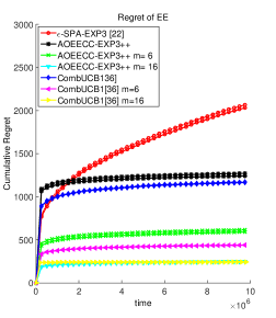
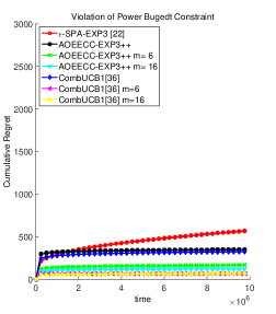
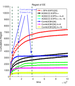
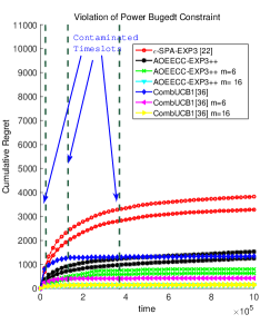
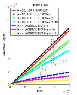
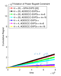
In Fig. 3, W.l.o.g., we normalize the EE into unitary value in every timeslot $n$. Then, we have $M=1$, $k=4$ and $K=32$. All computations of the collected datasets were conducted on an off-the-shelf desktop with dual $6$-core Intel i7 CPUs clocked at $2.66$Ghz. To show the advantages of our AOEECC-EXP3++ algorithms, we compare their performance to other existing MAB based algorithms, which includes: the EXP3 based combinatorial version (implemented by ourselves) of the $\epsilon$-SPA for non-stochastic MABs in CC [22], and we named it as “$\epsilon$-SPA-EXP3”; The combinatorial stochastic MAB algorithm, i.e., “CombUCB1”, with the tight regret bound as proved in [37], and the cooperative learning versions of algorithms of ours and others. In Fig. 3, the solid lines in the graphs represent the mean performance over the experiments and the dashed lines represent the mean plus on standard deviation (std) over the ten repetitions of the corresponding experiments. For a given optimal channel access strategy, small regret values indicate the large value of EE. We set all versions of our AOEECC-EXP3++ algorithms parameterized by ${\xi_{t}}(f)=\frac{{\ln(t{{\hat{\Delta}}_{t}}{{(f)}^{2}})}}{{32t{{\hat{\Delta}}_{t}}{{(f)}^{2}}}}$, where ${{{\hat{\Delta}}_{t}}(f)}$ is the empirical estimate of ${{{\Delta}_{t}}(f)}$, and parameters $\eta_{t}$ and $\delta_{t}$ according to the theorems.

In our first group of experiments in the stochastic regime (environment) as shown in Fig. 1(a), it is clear to see that AOEECC-EXP3++ enjoys almost the same (cumulative) regrets as CombUCB1 and has much lower regrets over time than the adversarial $\epsilon$-SPA-EXP3. We also see the significantly regrets reduction when accelerated learning ($m=6,16$) is employed for both AOEECC-EXP3++ and CombUCB1. For the subplot of the violation of budgeted constraint, we also see very similar behaviors among all algorithms for a fixed setting of the CC topology.

In our second group of experiments in the moderately contaminated stochastic environment, there are several contaminated timeslots as labeled in Fig. 1(b), which is made by irregular jamming behaviors at some rounds. In this case, the contamination does not make the whole dataset be fully adversarial, but drawn from a different stochastic model. Despite the corrupted rounds the AOEECC-EXP3++ algorithm successfully returns to the stochastic operation mode and achieves better results than $\epsilon$-SPA-EXP3 and has very close and comparable performance as CombUCB1. We also see the cooperative learning is highly efficient for all algorithms.

Refer to caption
Figure 4: EE loss of AOEECC-EXP3++ in a Path-loss Model

We conducted the third group of experiments in the adversarial regimes. We present the oblivious adversary case in Fig. 1(c). Due to the strong interference effect on each channel and the arbitrarily changing feature of the jamming behavior, all algorithms experience very high accumulated regrets. It can be find that our AOEECC-EXP3++ algorithm will have close and slightly worst learning performance when compared to $\epsilon$-SPA-EXP3, which confirms our theoretical analysis. Note that we do not implement stochastic MAB algorithms such as CombUCB1, since it is not applicable in this regime.

Refer to caption
Figure 5: EE loss of AOEECC-EXP3++ in Rician Distribution

In our fourth set of experiments shown in Fig. 1(d), we simulate the adaptive jamming attack case in the adversarial regime with a typical large memory $\Theta=20$. We can see large performance degradations for all algorithms when compared to the oblivious jammer case. The multiplicative effect of $\Theta$ makes the AOEECC-EXP3++ and $\epsilon$-SPA-EXP3 very hard to combat this type of jamming attack, although the regret curve is still sublinear after normalization.

Refer to caption
Figure 6: Measured EE in Different Regimes.

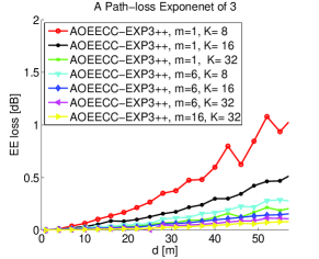
We also compare the average EE loss of the proposed AOEECC-EXP3++ algorithm (after a run of $10^{7}$ rounds) with respect to the optimal solution for 100 random channel realizations with a path-loss exponent of 3, a noise figure of 7 dB, a carrier frequency of 3.5 GHz, a noise bandwidth of 10 MHz, and the average circuit power $P_{c}^{t}(i_{f})$ = $29.2dBm$ for each transmitting channel $f$. The result is shown in Fig. 4. We can find that with the increasing of the number of available channels, the EE loss is decreasing. This confirms the well-known “multi-channel” diversity in wireless communications. In addition, increasing $m$ also reduces the average EE loss

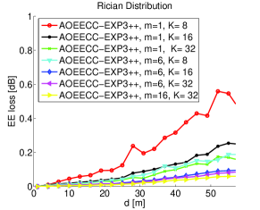
Moreoever, we conduct another group of experiment to verify the performance of our algorithms in the fading environments. We consider the Rician fading has a direct-to-scattered signal path ratio of $\bar{K}=6dB$, which is expected to dominate mobile communications. Fig. 5 shows the gaps between ours and optimal EE solutions, where we see similar phenomena but with a larger variance when compared with Fig. 4. Nevertheless, the figure shows that the results are reasonable for this typical conditions. It can be shown that the methodology presented in this paper can be applied to find the power allocation for any channel distribution for EECC.

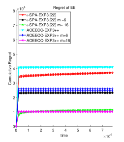
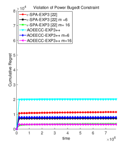
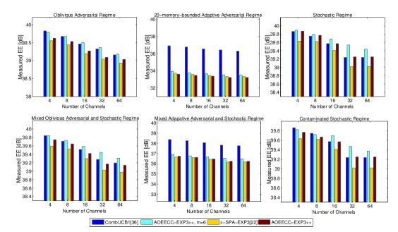
For brevity, we do not plot the regret performance figures for the mixed adversarial and stochastic regime. However, in our last experiments, we compare the measured EE (dB) for all the four different regimes after a relative long period of learning rounds $n=2*10^{7}$. We plot our results in Fig. 6. It is easy to find that our algorithm AOEECC-EXP3++ attains almost all the advantages of the stochastic MAB algorithms CombUCB1, and has better EE performance than $\epsilon$-SPA-EXP3.

X Conclusion

In this paper, we proposed the first adaptive multi-channel SPA algorithm for EECC without the knowledge about the nature of environments. At first, we captured features of general CC environments and divided them into four regimes, and then provided solid theoretical analysis for each of them. We find that our formulated constrained regret minimization problem requires joint control of learning rate and exploration parameters to achieve best performance. We have also found and verified that cooperative learning is an effective approach to improve the performance of EECC. Extensive simulations were conducted to verify the learning performance. The proposed algorithm could be implemented efficiently in practical CC with different sizes. We believe that the idea and algorithms of this paper can be applied to other wireless communications problems in unknown environments.

References

  • [1] G. P. Fettweis and E. Zimmermann, “ICT Energy Consumption-Trends and Challenges,” Proc. 11th Int. Symp. Wireless Personal Multimedia Commun. (WPMC 08), Lapland, Finland, Sept. 2008.
  • [2] S. Wang, F. Granelli, Y. Li, S. Chen, (Editors), “Energy-Efficient Cognitive Radio Networks,” special issue, IEEE Communications Magazine, vol.52, no.7, pp. 12 - 13, July, 2014.
  • [3] I. F. Akyildiz, W. Y. Lee, and K. R. Chowdhury, “CRAHNs: Cognitive radio ad hoc networks. AD hoc networks,” vol.7, no.5, pp. 810-836, 2009.
  • [4] I. F. Akyildiz, L. F. Brandon, and R. Balakrishnan, “Cooperative spectrum sensing in cognitive radio networks: A survey,” Physical communication, no. 1, pp. 40-62, 2011.
  • [5] I. Gomez-Miguelez, V. Marojevic, and A. Gelonch, “Energy-Efficient Water-Filling with Order Statistics,” IEEE Transactions on Vehicular Technology, vol.63, no.1, pp. 428-432, 2014.
  • [6] R. Fan, and H. Jiang, “Optimal multi-channel cooperative sensing in cognitive radio networks,” IEEE Transactions on Wireless Communications, vol. 9, no. 3, pp. 1128-1138, 2010.
  • [7] Q. Zhao, L. Tong, A. Swami, and Y. Chen, “Decentralized cognitive MAC for opportunistic spectrum access in ad hoc networks: A POMDP framework,” IEEE Journal on Selected Areas in Communications, vol.25, no.3, pp. 589-600, 2007
  • [8] B. Canberk, I. F. Akyildiz, S. Oktug, “Primary user activity modeling using first-difference filter clustering and correlation in cognitive radio networks,” IEEE/ACM Transactions on Networking (TON), vol.19, no.1, pp. 170-183, 2011
  • [9] W. Arbaugh, “Improving the latency of the probe phase during 802.11,” handoff, manuscript, 2009
  • [10] A. Anandkumar, N. Michael and A. Tang, “Opportunistic spectrum access with multiple users: learning under competition,” In Proc. of INFOCOM, pp. 1-9, 2010.
  • [11] Y. Gai, B. Krishnamachari and R. Jain, “Learning multiuser channel allocations in cognitive radio networks: A combinatorial multi-armed bandit formulation,” In IEEE Symposium on New Frontiers in Dynamic Spectrum (Dyspan), pp. 1-9, Aprial, 2010.
  • [12] K. Liu and Q. Zhao, “Distributed Learning in Multi-Armed Bandit with Multiple Players,” IEEE Transactions on Signal Processing, vol. 99, pp. 2234-2245, 2010.
  • [13] P. Zhou, Y. Chang, and J. Copeland, “Reinforcement learning for repeated power control game in cognitive radio networks,” IEEE Journal on Selected Areas in Communications, vol.30, no.1, pp. 54-69, 2012.
  • [14] B. Wang, Y.Wu, K. J. Liu, and T. Charles Clancy, “An anti-jamming stochastic game for cognitive radio networks,” IEEE Journal on Selected Areas in Communications, 29, no. 4, pp. 877-889, 2011.
  • [15] Y. Wu, B. Wang, K. J. Liu, and T. Charles Clancy, “Anti-jamming games in multi-channel cognitive radio networks,” IEEE Journal on Selected Areas in Communications, vol. 30, no. 1, pp. 4-15, 2012.
  • [16] H. Li, and Z. Han, “Dogfight in spectrum: jamming and anti-jamming in multichannel cognitive radio systems,” In IEEE Global Telecommunications Conference, IEEE GLOBECOM 2009, pp. 1-6, 2009.
  • [17] J. Oksanen, J. Lund n, and V. Koivunen, “Reinforcement learning based sensing policy optimization for energy efficient cognitive radio networks,” Neurocomputing, vol. 80, pp. 102-110, 2012.
  • [18] B. E. Veronica, and P. Mertikopoulos, “Energy-efficient power allocation in dynamic multi-carrier systems,” In VTC Spring, 2015.
  • [19] P. Mertikopoulos and B. E. Veronica, “ “Learning to be green: robust energy efficiency maximization in dynamic MIMO-OFDM systems, ” arXiv preprint arXiv:1504.03903, 2015, submitted to IEEE Journal on Selected Areas in Communications.
  • [20] S. Bubeck and N. Cesa-Bianchi, “Regret Analysis of Stochastic and Nonstochastic Multi-armed Bandit Problems,” Foundation and Trends in Machine Learning, vol. 5, 2012.
  • [21] Q. Wang, K. Ren, and P. Ning, “Anti-jamming communication in cognitive radio networks with unknown channel statistics,” in Proc. of IEEE ICNP 2011, pp. 393-402, 2011.
  • [22] X. Y. Li, P. Yang, Y. Yan, L. You, S. Tang and Q. Huang, “Almost optimal accessing of nonstochastic channels in cognitive radio networks ,” in Proc. of IEEE INFOCOM 2012, pp. 2291-2299, 2012.
  • [23] B. Li, P. Yang, J. Wang, Q. Wu, S. Tang, X.Y. Li, Y. Liu , “Almost Optimal Dynamically-Ordered Channel Sensing and Accessing for Cognitive Networks,” IEEE Transactions on Mobile Computing, pp.1203-1215, July, 2013.
  • [24] Y. Gai and B. Krishnamachari, “Decentralized Online Learning Algorithms for Opportunistic Spectrum Access,” in Proc. of IEEE GLOBECOM 2011, pp. 2534-2539, 2011.
  • [25] Q. Wang, P. Xu, K. Ren, and X. Y. Li, “ Towards optimal adaptive UFH-based anti-jamming wireless communication,” IEEE Journal on Selected Areas in Communications, vol. 99, no.1, pp. 16-30, 2012.
  • [26] A. Anandkumar, N.Michael, and A. K. Tang, “Opportunistic spectrum access withmultiple users: Learning under competition,” in Proc. of IEEE INFOCOM 2010, pp. 803-811, 2010.
  • [27] L. Lai, H. E. Gamal, H. Jiang, and H. V. Poor, “Cognitive medium access: Exploration, exploitation and competition,” IEEE Transactions on Mobile Computing, vol. 10, no. 2, pp. 239-253, 2007.
  • [28] K. Liu, and Q. Zhao, “Distributed learning in cognitive radio networks: Multi-armed bandit with distributed multiple players,” 2010 IEEE International Conference on Acoustics Speech and Signal Processing (ICASSP), pp. 3010-3013, 2010.
  • [29] R. Arora, D. Ofer, and T. Ambuj, “Online bandit learning against an adaptive adversary: from regret to policy regret,” In Proc. of ICML 2011, pp. 366-377, 2011.
  • [30] P. Zhou, T. Jiang, “Towards Optimal Adaptive Wireless Communications in Unknown Environments,” http://arxiv.org/abs/1505.06608
  • [31] O. Dekel, G. B. Ran, S. Ohad, and X. Lin, “Optimal distributed online prediction using mini-batches,” In Proc. of ICML 2012, pp. 58-70, 2012.
  • [32] T. L. Lai, and H. Robbins, “Asymptotically efficient adaptive allocation rules,” Advances in Applied Mathematics, 6, pp. 23-42, 1985.
  • [33] P. Auer, N. Cesa-Bianchi, Y. Freund, and R. E. Schapire, “The nonstochastic multiarmed bandit problem,” SIAM Journal on Computing, vol. 32, no.1, pp.48-77, 2002.
  • [34] S. Buccapatnam, J. Tan, and L. Zhang, “Information Sharing in Distributed Stochastic Bandits,” in Proc. of IEEE INFOCOM 2015, pp. 203-211, 2015.
  • [35] Y. Seldin, and A. Slivkins, “One practical algorithm for both stochastic and adversarial bandits,” In Proc. of ICML 2014, pp. 358-370, 2014.
  • [36] K. Liu and Q. Zhao, “Distributed learning in multi-armed bandit with multiple players,” IEEE Transactions on Signal Processing, vol. 58, no. 11, pp. 5667-5681, Nov. 2010.
  • [37] B. Kveton, Z. Wen, A. Ashkan, C. Szepesvari, “Tight Regret Bounds for Stochastic Combinatorial Semi-Bandits,” in Proc. of AISTATS 2015, pp. 535-543, 2015.
  • [38] A. Jean-Yves, B. S$\acute{a}$bastien, L. G$\acute{a}$bor, “Regret in Online Combinatorial Optimization,” Mathematics of Operations Research, vo.39, no.1, pp. 31-45, 2014.
  • [39] P. Auer, N. Cesa-Bianchi, and P. Fischer, “Finite-time analysis of the multiarmed bandit problem,” Machine learning, vol. 47, no. 2, pp. 235-256, 2002.
  • [40] A. G Barto. Reinforcement learning: An introduction. MIT press, 1998.
  • [41] M. Zinkevich, “Online Convex Programming and Generalized Infinitesimal Gradient Ascent,” In Proc. of ICML 2003, pp. 928-936, 2009.
  • [42] M. Pirmoradian,, O. Adigun, and C. Politis, “Adaptive power control scheme for energy efficient cognitive radio networks,” In IEEE International Conference on Communications (ICC 2012), pp. 6988-6992, 2012.
  • [43] M. Haddad, Y. Hayel, and O. Habachi, “Spectrum coordination in energy efficient cognitive radio networks,” IEEE Transactions on Vehicular Technology, , vol. 64. no.5, pp. 2112-2122, 2015.
  • [44] R. Xie, F. R. Yu, and H. Ji, “Energy-efficient spectrum sharing and power allocation in cognitive radio femtocell networks,” In IEEE INFOCOM 2012, pp. 1665-1673, 2012.
  • [45] R. Xie, F. R. Yu, H. Ji, and Yi Li, “Energy-efficient resource allocation for heterogeneous cognitive radio networks with femtocells,” IEEE Transactions on Wireless Communications, vol.11, no. 11, pp. 3910-3920, 2012.
  • [46] T. Jiang, C. Ni, D. Qu, and C. Wang, “Energy-efficient NC-OFDM/OQAM-based cognitive radio networks,” IEEE Communications Magazine, vol. 52, no. 7, pp. 54-60, 2014.
  • [47] A. Hasan, G. Bansal, E. Hossain, and V. K. Bhargava, “Energy-efficient power allocation in OFDM-based cognitive radio systems: A risk-return model,” IEEE Transactions on Wireless Communications, vol.8, no. 12, pp. 6078-6088, 2009.
  • [48] J. Wei, and Xi Zhang, “Energy-efficient distributed spectrum sensing for wireless cognitive radio networks,” In Proceedings IEEE INFOCOM, Workshops, pp. 1-6, 2010.
  • [49] Y. Seldin, P. Bartlett, K. Crammer, and Y. Abbasi-Yadkori, “ Prediction with Limited Advice and Multiarmed Bandits with Paid Observations,” In Proc. of ICML, pp. 280-287, 2014.
  • [50] S. Eryigit, S. Bayhan, and T. Tugcu, “Energy-efficient multichannel cooperative sensing scheduling with heterogeneous channel conditions for cognitive radio networks,” IEEE Transactions on Vehicular Technology, vol.62, no. 6, pp. 2690-2699, 2013.
[Uncaptioned image] Pan Zhou(S’07–M’14) is currently an associate professor with School of Electronic Information and Communications, Huazhong University of Science and Technology, Wuhan, P.R. China. He received his Ph.D. in the School of Electrical and Computer Engineering at the Georgia Institute of Technology (Georgia Tech) in 2011, Atlanta, USA. He received his B.S. degree in the Advanced Class of HUST, and a M.S. degree in the Department of Electronics and Information Engineering from HUST, Wuhan, China, in 2006 and 2008, respectively. He held honorary degree in his bachelor and merit research award of HUST in his master study. He was a senior technical member at Oracle Inc, America during 2011 to 2013, Boston, MA, USA, and worked on hadoop and distributed storage system for big data analytics at Oracle cloud Platform. His current research interest includes: wireless communication and networks, security and privacy, machine learning and big data.
[Uncaptioned image] Chenhui Hu(S’08) is currently pursuing his Ph.D. degree in engineering and applied sciences at Harvard University, Cambridge, MA. He is also a research assistant in the Center for Advanced Medical Imaging Sciences (CAMIS) of Massachusetts General Hospital. He received his B.S. and M.S. degrees in electronic engineering from Shanghai Jiao Tong University, Shanghai, China, in 2007 and 2010, respectively. He was a recipient of the Outstanding Graduates of Shanghai in 2010 and the 3rd IEEE ComSoc Asia-Pacific Outstanding Paper Award in 2014. His current research interests include mobile wireless communication, machine learning, statistical signal processing, and brain network analysis.
Tao Jiang (M’06–SM’10) is currently a full Professor in the School of Electronic Information and Communications, Huazhong University of Science and Technology, Wuhan, P. R. China. He received the B.S. and M.S. degrees in applied geophysics from China University of Geosciences, Wuhan, P. R. China, in 1997 and 2000, respectively, and the Ph.D. degree in information and communication engineering from Huazhong University of Science and Technology, Wuhan, P. R. China, in April 2004. From Aug. 2004 to Dec. 2007, he worked in some universities, such as Brunel University and University of Michigan-Dearborn, respectively. He has authored or co-authored over 160 technical papers in major journals and conferences and six books/chapters in the areas of communications and networks. He served or is serving as symposium technical program committee membership of some major IEEE conferences, including INFOCOM, GLOBECOM, and ICC, etc.. He is invited to serve as TPC Symposium Chair for the IEEE GLOBECOM 2013 and IEEEE WCNC 2013. He is served or serving as associate editor of some technical journals in communications, including in IEEE Communications Surveys and Tutorials, IEEE Transactions on Vehicular Technology, and IEEE Internet of Things Journal, etc.. He is a recipient of the NSFC for Distinguished Young Scholars Award in P. R. China. He is a senior member of IEEE.
Dapeng Oliver Wu (S’98–M’04–SM 06–F’13) received B.E. in Electrical Engineering from Huazhong University of Science and Technology, Wuhan, China, in 1990, M.E. in Electrical Engineering from Beijing University of Posts and Telecommunications, Beijing, China, in 1997, and Ph.D. in Electrical and Computer Engineering from Carnegie Mellon University, Pittsburgh, PA, in 2003. He is a professor at the Department of Electrical and Computer Engineering, University of Florida, Gainesville, FL. His research interests are in the areas of networking, communications, signal processing, computer vision, machine learning, smart grid, and information and network security. He received University of Florida Research Foundation Professorship Award in 2009, AFOSR Young Investigator Program (YIP) Award in 2009, ONR Young Investigator Program (YIP) Award in 2008, NSF CAREER award in 2007, the IEEE Circuits and Systems for Video Technology (CSVT) Transactions Best Paper Award for Year 2001, and the Best Paper Awards in IEEE GLOBECOM 2011 and International Conference on Quality of Service in Heterogeneous Wired/Wireless Networks (QShine) 2006. Currently, he serves as an Associate Editor for IEEE Transactions on Circuits and Systems for Video Technology, Journal of Visual Communication and Image Representation, and International Journal of Ad Hoc and Ubiquitous Computing. He is the founder of IEEE Transactions on Network Science and Engineering. He was the founding Editor-in-Chief of Journal of Advances in Multimedia between 2006 and 2008, and an Associate Editor for IEEE Transactions on Wireless Communications and IEEE Transactions on Vehicular Technology between 2004 and 2007. He is also a guest-editor for IEEE Journal on Selected Areas in Communications (JSAC), Special Issue on Cross-layer Optimized Wireless Multimedia Communications. He has served as Technical Program Committee (TPC) Chair for IEEE INFOCOM 2012, and TPC chair for IEEE International Conference on Communications (ICC 2008), Signal Processing for Communications Symposium, and as a member of executive committee and/or technical program committee of over 80 conferences. He has served as Chair for the Award Committee, and Chair of Mobile and wireless multimedia Interest Group (MobIG), Technical Committee on Multimedia Communications, IEEE Communications Society. He was a member of Multimedia Signal Processing Technical Committee, IEEE Signal Processing Society from Jan. 1, 2009 to Dec. 31, 2012. He is an IEEE Fellow.