Multilinear Map Layer: Prediction Regularization by Structural Constraint

1 Abstract

In this paper we propose and study a technique to impose structural constraints on the output of a neural network, which can reduce amount of computation and number of parameters besides improving prediction accuracy when the output is known to approximately conform to the low-rankness prior. The technique proceeds by replacing the output layer of neural network with the so-called MLM layers, which forces the output to be the result of some Multilinear Map, like a hybrid-Kronecker-dot product or Kronecker Tensor Product. In particular, given an “autoencoder” model trained on SVHN dataset, we can construct a new model with MLM layer achieving 62% reduction in total number of parameters and reduction of $\ell_{2}$ reconstruction error from 0.088 to 0.004. Further experiments on other autoencoder model variants trained on SVHN datasets also demonstrate the efficacy of MLM layers.

2 Introduction

To the human eyes, images made up of random values are typically easily distinguishable from those images of real world. In terms of Bayesian statistics, a prior distribution can be constructed to describe the likelihood of an image being a natural image. An early example of such “image prior” is related to the frequency spectrum of an image, which assumes that lower-frequency components are generally more important than high-frequency components, to the extent that one can discard some high-frequency components when reducing the storage size of an image, like in JPEG standard of lossy compression of images (Wallace, 1991).

Another family of image prior is related to the so called sparsity pattern(Candes et al., 2006, Candès et al., 2006, Candes et al., 2008), which refers to the phenomena that real world data can often be constructed from a handful of exemplars modulo some negligible noise. In particular, for data represented as vector $\bf{d}\in{\mathbb{F}}^{m}$ that exhibits sparsity, we can construct the following approximation:

$$\bf{d}\approx{\bf D}{\bf x}\text{,}$$ (1)

where ${\bf D}\in{\mathbb{F}}^{m\times n}$ is referred to as dictionary for $\bf{d}$ and ${\bf x}$ is the weight vector combining rows of the dictionary to reconstruct $\bf{d}$. In this formulation, sparsity is reflected by the phenomena that number of non-zeros in ${\bf x}$ is often much less than its dimension, namely:

$$\|{\bf x}\|_{0}\ll m\text{.}$$ (2)

The sparse representation ${\bf x}$ may be derived in the framework of dictionary learning(Olshausen and Field, 1997, Mairal et al., 2009) by the following optimization:

$$\min_{\bf x}\|{\bf M}-\sum_{i}x_{i}{\bf D}_{i}\|_{F}+\lambda f({\bf x})\text{,}$$ (3)

where ${\bf D}_{i}$ is a component in dictionary, $f$ is used to induce sparsity in ${\bf x}$, with $\ell_{1}$ being a possible choice.

2.1 Low-Rankness as Sparse Structure in Matrices

When data is represented as a matrix ${\bf M}$, the formulation of 3 is related to the rank of ${\bf M}$ by Theorem LABEL:thm:svd-opt in the following sense:

$$\operatorname{rank}({\bf M}) =\min_{{\bf x}}\|{\bf x}\|_{0}$$ (4)

$$\text{ s.t. }{\bf M}=\sum_{i}x_{i}{\bf D}_{i},$$ (5)

$${\bf D}_{i}={\bf u}_{i}\bf{v}_{i}^{\top},\,{\bf u}_{i}^{\top}{\bf u}_{i}=1,\,\bf{v}_{i}^{\top}\bf{v}_{i}=1\text{.}$$ (6)

Hence a low rank matrix ${\bf M}$ always has a sparse representation w.r.t. some rank-1 orthogonal bases. This unified view allows us to generalize the sparsity pattern to images by requiring the underlying matrix to be low-rank.

When an image has multiple channels, it may be represented as a tensor ${\mathcal{T}}\in{\mathbb{F}}^{C\times H\times W}$ of order 3. Nevertheless, the matrix structure can still be recovered by unfolding the tensor along some dimension.

In Figure 1, it is shown that the unfolding of the RGB image tensor along the width dimension can be well approximated by a low-rank matrix as energy is concentrated in the first few components.

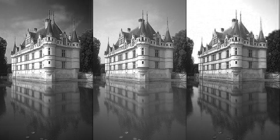
(a) The unfolding of an RGB sample image.

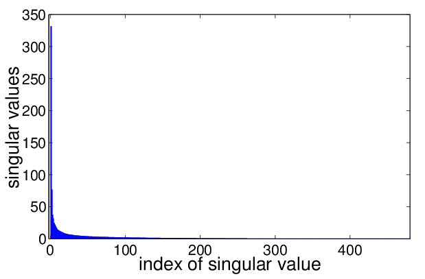
(b) The singular values

Figure 1: An illustration of the singular values of the unfolding of an RBG sample image.

In particular, given Singular Value Decomposition of a matrix ${\bf M}={\bf U}{\bf D}{\bf V}^{*}$, where ${\bf U},{\bf V}$ are unitary matrices and ${\bf D}$ is a diagonal matrix with the diagonal made up of singular values of ${\bf M}$, a rank-$k$ approximation of ${\bf M}\in{\mathbb{F}}^{m\times n}$ is:

$${\bf M}\approx{\bf M}_{k}=\tilde{{\bf U}}\tilde{{\bf D}}\tilde{{\bf V}}^{*},\,\tilde{{\bf U}}\in{\mathbb{F}}^{m\times k}\text{, }\tilde{{\bf D}}\in{\mathbb{F}}^{k\times k}\text{, }\tilde{{\bf V}}\in{\mathbb{F}}^{n\times k}\text{,}$$ (7)

where $\tilde{{\bf U}}$ and $\tilde{{\bf V}}$ are the first $k$-columns of the ${\bf U}$ and ${\bf V}$ respectively, and $\tilde{{\bf D}}$ is a diagonal matrix made up of the largest $k$ entries of ${\bf D}$.

In this case approximation by SVD is optimal in the sense that the following holds (Horn and Johnson, 1991):

$${\bf M}_{r}=\inf_{{\bf X}}\|{\bf X}-{\bf M}\|_{F}\text{ s.t. }\operatorname{rank}({\bf X})\leq r\text{,}$$ (8)

and

$${\bf M}_{r}=\inf_{{\bf X}}\|{\bf X}-{\bf M}\|_{2}\text{ s.t. }\operatorname{rank}({\bf X})\leq r\text{.}$$ (9)

An important variation of the SVD-based low rank approximation is to also model the $\ell_{1}$ noise in the data:

$$\|{\bf M}\|_{RPCA}=\inf_{{\bf S}}\|{\bf M}-{\bf S}\|_{*}+\lambda\|{\bf S}\|_{1}\text{.}$$ (10)

This norm which we tentatively call “RPCA-norm” (Candès et al., 2011), is well-defined as it is infimal convolution (Rockafellar, 2015) of two norms.

2.2 Low Rank Structure for Tensor

Above, we have used the low-rank structure of the unfolded matrix of a rank-3 tensor corresponding to RGB values of an image to reflect the low rank structure of the tensor. However, there are multiple ways to construct of matrix ${\bf D}\in{\mathbb{R}}^{m\times 3n}$, e.g., by stacking ${\bf R}$, ${\bf G}$ and ${\bf B}$ together horizontally. An emergent question is if we construct a matrix ${\bf D}^{\prime}\in{\mathbb{R}}^{3m\times n}$ by stacking ${\bf R}$, ${\bf G}$ and ${\bf B}$ together vertically. Moreover, it would be interesting to know if there is a method that can exploit both forms of constructions. It turns out that we can deal with the above variation by enumerating all possible unfoldings. For example, the nuclear norm of a tensor may be defined as:

Definition 1

Given a tensor ${\mathcal{E}}$, let ${\bf E}_{(i)}=\operatorname{fold}^{-1}_{i}({\mathcal{E}})$ be unfolding of ${\mathcal{E}}$ to matrices. The nuclear norm of ${\mathcal{E}}$ is defined w.r.t. some weights $\beta_{i}$ (satisfying $\beta_{i}\geq 0$) as a weighted sum of the matrix nuclear norms of unfolded matrices ${\bf E}_{(i)}$ as:

$$\|{\mathcal{E}}\|{*}=\sum_{i}\beta_{i}\|{\bf E}_{(i)}\|{*}\textrm{.}$$ (11)

Consequently, minimizing the tensor nuclear norm will minimize the matrix nuclear norm of all unfoldings of tensor. Further, by adjusting the weights used in the definition of the tensor nuclear norm, we may selectively minimize the nuclear norm of some unfoldings of the tensor.

2.3 Stronger Sparsity for Tensor by Kronecker Product Low Rank

When an image is taken as matrix, the basis for low rank factorizations are outer products of row and column vectors. However, if data exhibits Principle of Locality, then only adjacent rows and columns can be meaningfully related, meaning the rank in this decomposition will not be too low. In contrast, local patches may be used as basis for low rank structure (Elad and Aharon, 2006, Yang et al., 2008, Schaeffer and Osher, 2013, Dong et al., 2014b, Yoon et al., 2014). Further, patches may be grouped before assumed to be of low-rank (Buades et al., 2005, Hu et al., 2015, Kwok, 2015).

A simple method to exploit the low-rank structure of the image patches is based on Kronecker Product SVD of matrix ${\bf M}\in{\mathbb{F}}^{m\times n}$:

$${\bf M}=\sum_{i=1}^{\operatorname{rank}(\mathscr{R}({\bf M}))}\sigma_{i}{\bf U}_{i}\otimes{\bf V}_{i}\text{,}$$ (12)

where $\mathscr{R}({\bf A})$ is the operator defined in (Van Loan, 2000, Van Loan et al., 1993) which shuffles indices.

$$\mathscr{R}({\bf A}\otimes{\bf B})=\operatorname{vec}{{\bf A}}(\operatorname{vec}{{\bf B}})^{\top}\text{.}$$ (13)

Note that outer product is a special case of Kronecker product when ${\bf A}\in{\mathbb{F}}^{m\times 1}$ and ${\bf B}\in{\mathbb{F}}^{1\times n}$, hence we have SVD as a special case of KPSVD. The choice of shapes of ${\bf A}$ and ${\bf B}$, however, affects the extent to which the underlying sparsity assumption is valid. Below we give an empirical comparison of a KPSVD with SVD. The image is of width 480 and height 320, and we approximate the image with KPSVD and SVD respectively for different ranks. To make the results comparable, we let ${\bf B}\in{\mathbb{F}}^{16x20}$ to make the number of parameters in two approach equal.

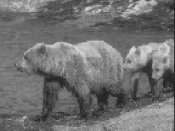
(a) Original image selected from BSD500 dataset(Arbelaez et al., 2011)

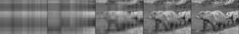
(b) SVD approximations with rank 1, 2, 5, 10, 20 respectively from left to right

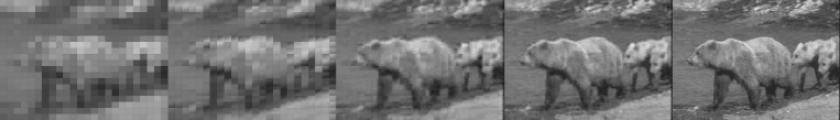
(c) KPSVD approximations with right matrix having shape 16x20 and with rank 1, 2, 5, 10, 20 respectively from left to right

Figure 2: This figures visually compares the results of KPSVD and SVD approximation given the same number of parameters. For this example, it can be seen that KPSVD with right matrix shape 16x20 is considerably better than SVD in approximation.

We may extend Kronecker product to tensors as Kronecker Tensor Product as:

Definition 2

Kronecker tensor product(Phan et al., 2013, 2012) is defined for two tensors of the same order $k$. I.e., for two tensors:

$$\mathcal{A}\in{\mathbb{F}}^{m_{1}\times m_{2},\cdots,\times m_{k}}\text{,}$$ (14)

and

$$\mathcal{B}\in{\mathbb{F}}^{n_{1}\times n_{2},\cdots,\times n_{k}}\text{,}$$ (15)

we define Kronecker product of tensor as

$$(\mathcal{A}\otimes\mathcal{B})_{i_{1},i_{2},\cdots,i_{k}}\coloneqq A_{\lfloor i_{1}/m_{1}\rfloor,\lfloor i_{2}/m_{2}\rfloor,\cdots,\lfloor i_{k}/m_{k}\rfloor}B_{i_{1}\bmod m_{1},i_{2}\bmod m_{2},\cdots,i_{k}\bmod m_{k}}$$ (16)

where

$$\mathcal{A}\otimes\mathcal{B}\in{\mathbb{F}}^{m_{1}n_{1}\times m_{2}n_{2},\cdots,\times m_{k}n_{k}}\text{.}$$ (17)

With the help of Kronecker Tensor Product, (Phan et al., 2013, 2012) is able to extend KPSVD to tensors as:

$${\mathcal{T}}=\sum_{i=1}^{\operatorname{rank}(\mathscr{R}({\mathcal{T}}))}\sigma_{i}\mathcal{U}_{i}\otimes\mathcal{V}_{i}\text{,}$$ (18)

where $\mathscr{R}({\mathcal{T}})$ is a matrix.

3 Prediction Regularization by Structural Constraint

In a neural network like

$$\inf_{\theta}d({\bf Y},f({\bf X};\theta))\text{,}$$ (19)

If $f({\bf X};\theta)$, the prediction of the network, is known to be like an image, it is desirable to use the image priors to help improve the prediction quality. An example of such a neural network is the so-called “Autoencoder” (Vincent et al., 2008, Deng et al., 2010, Vincent et al., 2010, Ng, 2011), which when presented with a possibly corrupted image, will output a reconstructed image that possibly have the noise suppressed.

One method to exploit the prior information is to introduce an extra cost term to regularize the output as

$$\inf_{\theta}d({\bf Y},{\bf Z})+\lambda r({\bf Z})\text{ s.t. }{\bf Z}=f({\bf X};\theta)\text{,}$$ (20)

The regularization technique is well studied in the matrix and tensor completion literature (Liu et al., 2013, Tomioka et al., 2010, Gandy et al., 2011, Signoretto et al., 2011, Kressner et al., 2013, Bach et al., 2012). For example, nuclear norm $\|{\bf Z}\|_{*}$, which is sum of singular values, or logarithm of determinant $\log(\det(\epsilon{\bf I}+{\bf Z}{\bf Z}^{\top}))$ (Fazel et al., 2003), may be used to induce low-rank structure if ${\bf Z}$ is a matrix. It is even possible to use RPCA-norm to better handle the possible sparse non-low-rank components in ${\bf Z}$ by letting $r({\bf Z})=\|{\bf Z}\|_{RPCA}$.

However, using extra regularization terms also involve a few subtleties:

1. The training of neural network incurs extra cost of computing the regularizer terms, which slows down training. This impact is exacerbated if the regularization terms cannot be efficiently computed in batch, like when using the nuclear norm or RPCA-norm regularizers together with the popular mini-batch based Stochastic Gradient Descent training algorithm (Bottou, 2010).

2. The value of $\lambda$ is application-specific and may only be found through grid search on validation set. For example, when $r$ reflects low-rankness of the prediction, larger value of $\lambda$ may induce result of lower-rank, but may cause degradation of the reconstruction quality.

We take an alternative method by directly restricting the parameter space of the output. Assume in the original neural network, the output is given by a Fully-Connected (FC) layer as:

$${\bf L}_{a}=h({\bf L}_{a-1}{\bf M}_{a}+{\bf b}_{a})\text{.}$$ (21)

It can be seen that the output ${\bf L}_{a}\in{\mathbb{F}}^{m\times n}$ has $mn$ number of free parameters. However, noting that the product of two matrices ${\bf A}\in{\mathbb{F}}^{m\times r}$ and ${\bf B}\in{\mathbb{F}}^{r\times n}$ will have the property

$$\operatorname{rank}({\bf A}{\bf B})\leq r\text{,}$$ (22)

when $m\geq r$ and $n\geq r$.

Hence we may enforce that $\operatorname{rank}({\bf L}_{a})\leq r$ by the following construct for example:

$${\bf L}_{a}=h({\bf L}_{a-1}{\bf M}_{a}+{\bf b}_{a})h({\bf L}_{a-1}{\bf N}_{a}+{\bf c}_{a})\text{,}$$ (23)

when we have:

$${\bf L}_{a-1}{\bf M}_{a}+{\bf b}_{a}\in{\mathbb{F}}^{m\times r}$$ (24)

$${\bf L}_{a-1}{\bf N}_{a}+{\bf c}_{a}\in{\mathbb{F}}^{r\times n}\text{.}$$ (25)

In a Convolutional Neural Network where intermediate data are represented as tensors, we may enforce the low-rank image prior similarly. In fact, by proposing a new kind of output layer to explicitly encode the low-rankness of the output based on some kinds of Multilinear Map, like a hybrid of Kronecker and dot product, or Kronecker tensor product, we are able to increase the quality of denoising and reduce amount of computation at the same time. We outline the two formulations below.

Assume each output instance of a neural network is an image represented by a tensor of order 3:

$${\mathcal{T}}\in{\mathbb{F}}^{C\times H\times W}\text{,}$$ (26)

where $C$, $H$ and $W$ are number of channels, height and width of the image respectively.

3.1 KTP layer

In KTP layers, we approximate ${\mathcal{T}}$ by Kronecker Tensor Product of two tensors.

$${\mathcal{T}}\approx\mathcal{A}\otimes\mathcal{B}\text{.}$$ (27)

As by applying the shuffle operator defined in (Van Loan, 2000, Van Loan et al., 1993), 28 is equivalent to:

$$\mathscr{R}({\mathcal{T}})\approx\operatorname{vec}{\mathcal{A}}\operatorname{vec}{\mathcal{B}}^{\top}\text{,}$$ (28)

hence we are effectively doing rank-1 approximation of the matrix $\mathscr{R}({\mathcal{T}})$. A natural extension would then be to increase the number of components in approximation as:

$${\mathcal{T}}\approx\sum_{i=1}^{K}\mathcal{A}_{i}\otimes\mathcal{B}_{i}\text{.}$$ (29)

We may further combine the multiple shape formulation of 29 to get the general form of KTP layer:

$${\mathcal{T}}\approx\sum_{j=1}^{J}\sum_{i=1}^{K}{\mathcal{A}}_{ij}\otimes{\mathcal{B}}_{ij}\text{.}$$ (30)

where $\{{\mathcal{A}}_{ij}\}_{i=1}^{K}$ and $\{{\mathcal{B}}_{i,j}\}_{i=1}^{K}$ are of the same shape respectively.

3.2 HKD layer

In HKD layers, we approximate ${\mathcal{T}}$ by the following multilinear map between $\mathcal{A}\in{\mathbb{F}}^{C_{1}\times H_{1}\times W_{1}}$ and $\mathcal{B}\in{\mathbb{F}}^{C_{1}\times C_{2}\times H_{2}\times W_{2}}$, which is a hybrid of Kronecker product and dot product:

$$T_{c,h,w}\approx\tilde{T}_{c,h,w}=\tilde{T}_{c,h_{1}+H_{1}*h_{2},w_{1}+W_{1}*w_{2}}=\sum_{c_{1}}A_{c_{1},h_{2},w_{2}}B_{c,c_{1},h_{1},w_{1}}\text{,}$$ (31)

where $h=h_{1}h_{2}$, $w=w_{1}w_{2}$.

The rationale behind this construction is that the Kronecker product along the spatial dimension of $H$ and $W$ may capture the spatial regularity of the output, which enforces low-rankness; while the dot product along $C$ would allow combination of information from multiple channels of $\mathcal{A}$ and $\mathcal{B}$.

In the framework of low-rank approximation, the formulation 31 is by no means unique. One could for example improve the precision of approximation by introducing multiple components as:

$$T_{c,h,w}=T_{c,h_{1}+H_{1}*h_{2},w_{1}+W_{1}*w_{2}}\approx\sum_{k}\sum_{c_{1}}A_{k,c_{1},h_{2},w_{2}}B_{k,c,c_{1},h_{1},w_{1}}\text{.}$$ (32)

Hereafter we would refer to layers constructed following 31 as HKD layers. The general name of MLM layers will refer to all possible kinds of layers that can be constructed from other kinds of multilinear map.

3.3 General MLM layer

A Multilinear map is a function of several variables that is linear separately in each variable as:

$$f\colon V_{1}\times\cdots\times V_{n}\to W\text{,}$$ (33)

where $V_{1},\ldots,V_{n}$ and $W\!$ are vector spaces with the following property: for each $i\!$, if all of the variables but $v_{i}\!$ are held constant, then $f(v_{1},\ldots,v_{n})$ is a linear function of $v_{i}\!$(Lang, 2002). It is easy to verify that Kronecker product, convolution, dot product are all special cases of multilinear map.

Figure 3 gives a schematic view of general structure of the MLM layer. The left factor and right factor are produced from the same input, which are later combined by the multilinear map to produce the output. Depending on the type of multilinear map used, the MLM layer will become HKD layer or KTP layer. We note that it is also possible to introduce more factors than two into an MLM layer.

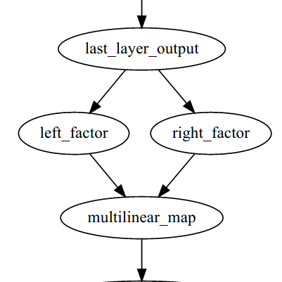
Figure 3: Diagram of the structure of a MLM layer. the output of the preceding layer is fed into two nodes where left factor tensor and right factor tensor are computed. Then a multilinear map is applied on the left and right factors to construct the output.

4 Empirical Evaluation of Multilinear Map Layer

We next empirically study the properties and efficacy of the Multilinear Map layers and compare it with the case when no structural constraint is imposed on the output.

To make a fair comparison, we first train a covolutional autoencoder with the output layer being a fully-connected layer as a baseline. Then we replace the fully-connected layer with different kinds of MLM layers and train the new network until quality metrics stabilizes. For example, Figure 4 gives a subjective comparison of HKD layer with the original model on SVHN dataset. We then compare MLM layer method with the baseline model in terms of number of parameters and prediction quality. We do the experiments based on implementation of MLM layers in Theano(Bergstra et al., 2010, Bastien et al., 2012) framework.

(a) Original image patches selected from SVHN dataset

(b) Results of an Autoencoder A1

(c) Results of an Autoencoder A2 with less neurons in the bottleneck layer than A1

(d) Results of an Autoencoder with as many neurons in the bottleneck layer as A2 but uses HKD as output layer

Figure 4: This figures show the results of passing five cropped patched from SVHN dataset as input images through Autoencoders with different output layers. The first row contains the original images. The second row contains the output of an Autoencoder “A1”. The third row contains the output of an Autoencoder “A2”, which has smaller number of hidden units in the bottleneck layer. The fourth row contains the output of an Autoencoder “A3” constructed from “A2” by replacing the output FC layer with a HKD layer. It can be seen that “A3”, though with smaller number of hidden units in bottleneck layer, visually performs better than “A1” and “A2” in reconstruting the input images.

Table 1: Evaluation of MLM layers on SVHN digit reconstruction

model	bottleneck #hidden unit	total #params	layer #params	L2 error
conv + FC	512	13.33M	5764800	3.4e-2
conv + HKD	512	4.97M	46788	5.2e-4
conv + HKD multiple components	512	5.05M	118642	3.6e-4
conv + FC	64	13.40M	5764800	1.3e-1
conv+ HKD	64	5.04M	46788	1.8e-3
conv + KTP	64	5.04M	46618	3.2e-3
conv	16	5.09M	0	4.0e-2
conv + FC	16	13.36M	5764800	8.8e-2
conv + HKD	16	5.00M	46788	3.8e-3
conv + KTP	16	5.00M	46618	5.8e-3

Table 1 shows the performance of MLM layers on training an autoencoder for SVHN digit reconstruction. The network first transforms the $40\times 40$ input image to a bottleneck feature vector through a traditional ConvNet consisting of 4 convolutional layers, 3 max pooling layers and 1 fully connected layer. Then, the feature is transformed again to reconstruct the image through 4 convolutional layers, 3 un-pooling layers and the last fully-connected layer or its alternatives as output layer. The un-pooling operation is implemented with the same approach used in (Dosovitskiy et al., 2014), by simply setting the pooled value at the top-left corner of the pooled region, and leaving other as zero. The fourth column of the table is the number of parameters in fully-connected layer or its alternative MLM layer. By varying the length of bottleneck feature and using different alternatives for FC layer, we can observe that both HKD and KTP layer are good alternatives for FC layer as output layer, and they also both significantly reduce the number of parameters. We also tested the case with convolutional layer as output layer, and the result still shows the efficacy of MLM layer.

As the running time may depend on particular implementation details of the KFC and the Theano framework, we do not report running time. However, the complexity analysis suggests that there should be significant reduction in amount of computation.

5 Related Work

In this section we discuss related work not covered in previous sections.

Low rank approximation has been a standard tool in restricting the space of the parameters. Its application in linear regression dates back to (Anderson, 1951). In (Sainath et al., 2013, Liao et al., 2013, Xue et al., 2013, Zhang et al., 2014b, Denton et al., 2014), low rank approximation of fully-connected layer is used; and (Jaderberg et al., 2014, Rigamonti et al., 2013, Lebedev et al., 2014b, a, Denil et al., 2013) also considered low rank approximation of convolution layer. (Zhang et al., 2014a) considered approximation of multiple layers with nonlinear activations. To our best knowledge, these methods only consider applying low-rank approximation to weights of the neural network, but not to the output of the neural network.

As structure is a general term, there are also other types of structure that exist in the desired prediction. Neural network with structured prediction also exist for tasks other than autoencoder, like edge detection(Dollár and Zitnick, 2013), image segmentation(Zheng et al., 2015, Farabet et al., 2013), super resolution(Dong et al., 2014a), image generation(Dosovitskiy et al., 2014). The structure in these problem may also exhibit low-rank structure exploitable by MLM layers.

6 Conclusion and Future Work

In this paper, we propose and study methods for incorporating the low-rank image prior to the predictions of the neural network. Instead of using regularization terms in the objective function of the neural network, we directly encode the low-rank constraints as structural constraints by requiring the output of the network to be the result of some kinds of multilinear map. We consider a few variants of multilinear map, including a hybrid-Kronecker-dot product and Kronecker tensor product. We have found that using the MLM layer can significantly reduce the number of parameters and amount of computation for autoencoders on SVHN.

As future work, we note that when using $\ell_{1}$ norm as objective together with the structural constraint, we could effectively use the norm defined in Robust Principal Value Analysis as our objective, which would be able to handle the sparse noise that may otherwise degrade the low-rankness property of the predictions. In addition, it would be interesting to investigate applying the structural constraints outlined in this paper to the output of intermediate layers of neural networks.

References

- Anderson (1951) Theodore Wilbur Anderson. Estimating linear restrictions on regression coefficients for multivariate normal distributions. The Annals of Mathematical Statistics, pages 327–351, 1951.
- Arbelaez et al. (2011) Pablo Arbelaez, Michael Maire, Charless Fowlkes, and Jitendra Malik. Contour detection and hierarchical image segmentation. IEEE Trans. Pattern Anal. Mach. Intell., 33(5):898–916, May 2011. ISSN 0162-8828. doi: 10.1109/TPAMI.2010.161. URL http://dx.doi.org/10.1109/TPAMI.2010.161.
- Bach et al. (2012) Francis Bach, Rodolphe Jenatton, Julien Mairal, and Guillaume Obozinski. Optimization with sparsity-inducing penalties. Found. Trends Mach. Learn., 4(1):1–106, January 2012. ISSN 1935-8237. doi: 10.1561/2200000015. URL http://dx.doi.org/10.1561/2200000015.
- Bastien et al. (2012) Frédéric Bastien, Pascal Lamblin, Razvan Pascanu, James Bergstra, Ian J. Goodfellow, Arnaud Bergeron, Nicolas Bouchard, and Yoshua Bengio. Theano: new features and speed improvements. Deep Learning and Unsupervised Feature Learning NIPS 2012 Workshop, 2012.
- Bergstra et al. (2010) James Bergstra, Olivier Breuleux, Frédéric Bastien, Pascal Lamblin, Razvan Pascanu, Guillaume Desjardins, Joseph Turian, David Warde-Farley, and Yoshua Bengio. Theano: a CPU and GPU math expression compiler. In Proceedings of the Python for Scientific Computing Conference (SciPy), June 2010. Oral Presentation.
- Bottou (2010) Léon Bottou. Large-scale machine learning with stochastic gradient descent. In Proceedings of COMPSTAT’2010, pages 177–186. Springer, 2010.
- Buades et al. (2005) Antoni Buades, Bartomeu Coll, and Jean-Michel Morel. Image denoising by non-local averaging. In ICASSP (2), pages 25–28, 2005.
- Candès et al. (2011) Emmanuel Candès, Xiaodong Li, Yi Ma, and John Wright. Robust principal component analysis. Journal of the ACM, 58(3), May 2011.
- Candès et al. (2006) Emmanuel J Candès, Justin Romberg, and Terence Tao. Robust uncertainty principles: Exact signal reconstruction from highly incomplete frequency information. Information Theory, IEEE Transactions on, 52(2):489–509, 2006.
- Candes et al. (2006) Emmanuel J Candes, Justin K Romberg, and Terence Tao. Stable signal recovery from incomplete and inaccurate measurements. Communications on pure and applied mathematics, 59(8):1207–1223, 2006.
- Candes et al. (2008) Emmanuel J Candes, Michael B Wakin, and Stephen P Boyd. Enhancing sparsity by reweighted ℓ 1 minimization. Journal of Fourier analysis and applications, 14(5-6):877–905, 2008.
- Deng et al. (2010) Li Deng, Michael L Seltzer, Dong Yu, Alex Acero, Abdel-rahman Mohamed, and Geoffrey E Hinton. Binary coding of speech spectrograms using a deep auto-encoder. In Interspeech, pages 1692–1695. Citeseer, 2010.
- Denil et al. (2013) Misha Denil, Babak Shakibi, Laurent Dinh, Nando de Freitas, et al. Predicting parameters in deep learning. In Advances in Neural Information Processing Systems, pages 2148–2156, 2013.
- Denton et al. (2014) Emily L Denton, Wojciech Zaremba, Joan Bruna, Yann LeCun, and Rob Fergus. Exploiting linear structure within convolutional networks for efficient evaluation. In Advances in Neural Information Processing Systems, pages 1269–1277, 2014.
- Dollár and Zitnick (2013) Piotr Dollár and C Lawrence Zitnick. Structured forests for fast edge detection. In Computer Vision (ICCV), 2013 IEEE International Conference on, pages 1841–1848. IEEE, 2013.
- Dong et al. (2014a) Chao Dong, Chen Change Loy, Kaiming He, and Xiaoou Tang. Image super-resolution using deep convolutional networks. arXiv preprint arXiv:1501.00092, 2014a.
- Dong et al. (2014b) Weisheng Dong, Guangming Shi, Xin Li, Yi Ma, and Feng Huang. Compressive sensing via nonlocal low-rank regularization. Image Processing, IEEE Transactions on, 23(8):3618–3632, 2014b.
- Dosovitskiy et al. (2014) Alexey Dosovitskiy, Jost Tobias Springenberg, and Thomas Brox. Learning to generate chairs with convolutional neural networks. arXiv preprint arXiv:1411.5928, 2014.
- Elad and Aharon (2006) Michael Elad and Michal Aharon. Image denoising via sparse and redundant representations over learned dictionaries. Image Processing, IEEE Transactions on, 15(12):3736–3745, 2006.
- Farabet et al. (2013) Clement Farabet, Camille Couprie, Laurent Najman, and Yann LeCun. Learning hierarchical features for scene labeling. Pattern Analysis and Machine Intelligence, IEEE Transactions on, 35(8):1915–1929, 2013.
- Fazel et al. (2003) Maryam Fazel, Haitham Hindi, and Stephen P Boyd. Log-det heuristic for matrix rank minimization with applications to hankel and euclidean distance matrices. In American Control Conference, 2003. Proceedings of the 2003, volume 3, pages 2156–2162. IEEE, 2003.
- Gandy et al. (2011) Silvia Gandy, Benjamin Recht, and Isao Yamada. Tensor completion and low-n-rank tensor recovery via convex optimization. Inverse Problems, 27(2):025010, 2011.
- Horn and Johnson (1991) Roger A Horn and Charles R Johnson. Topics in matrix analysis. Cambridge university press, 1991.
- Hu et al. (2015) Haijuan Hu, Jacques Froment, and Quansheng Liu. Patch-based low-rank minimization for image denoising. arXiv preprint arXiv:1506.08353, 2015.
- Jaderberg et al. (2014) Max Jaderberg, Andrea Vedaldi, and Andrew Zisserman. Speeding up convolutional neural networks with low rank expansions. arXiv preprint arXiv:1405.3866, 2014.
- Kressner et al. (2013) Daniel Kressner, Michael Steinlechner, and Bart Vandereycken. Low-rank tensor completion by riemannian optimization. BIT Numerical Mathematics, pages 1–22, 2013.
- Kwok (2015) Quanming Yao James T Kwok. Colorization by patch-based local low-rank matrix completion. 2015.
- Lang (2002) Serge Lang. Algebra revised third edition. GRADUATE TEXTS IN MATHEMATICS-NEW YORK-, 2002.
- Lebedev et al. (2014a) Vadim Lebedev, Yaroslav Ganin, Maksim Rakhuba, Ivan Oseledets, and Victor Lempitsky. Speeding-up convolutional neural networks using fine-tuned cp-decomposition. arXiv preprint arXiv:1412.6553, 2014a.
- Lebedev et al. (2014b) Vadim Lebedev, Yaroslav Ganin, Maksim Rakhuba, Ivan V. Oseledets, and Victor S. Lempitsky. Speeding-up convolutional neural networks using fine-tuned cp-decomposition. CoRR, abs/1412.6553, 2014b. URL http://arxiv.org/abs/1412.6553.
- Liao et al. (2013) Hank Liao, Erik McDermott, and Andrew Senior. Large scale deep neural network acoustic modeling with semi-supervised training data for youtube video transcription. In Automatic Speech Recognition and Understanding (ASRU), 2013 IEEE Workshop on, pages 368–373. IEEE, 2013.
- Liu et al. (2013) Ji Liu, Przemyslaw Musialski, Peter Wonka, and Jieping Ye. Tensor completion for estimating missing values in visual data. IEEE Trans. Pattern Anal. Mach. Intell., 35(1):208–220, January 2013. ISSN 0162-8828. doi: 10.1109/TPAMI.2012.39. URL http://dx.doi.org/10.1109/TPAMI.2012.39.
- Mairal et al. (2009) Julien Mairal, Jean Ponce, Guillermo Sapiro, Andrew Zisserman, and Francis R Bach. Supervised dictionary learning. In Advances in neural information processing systems, pages 1033–1040, 2009.
- Ng (2011) Andrew Ng. Sparse autoencoder. CS294A Lecture notes, 72, 2011.
- Olshausen and Field (1997) Bruno A Olshausen and David J Field. Sparse coding with an overcomplete basis set: A strategy employed by v1? Vision research, 37(23):3311–3325, 1997.
- Phan et al. (2012) Anh Huy Phan, Andrzej Cichocki, Petr Tichavskỳ, Danilo P Mandic, and Kiyotoshi Matsuoka. On revealing replicating structures in multiway data: A novel tensor decomposition approach. In Latent Variable Analysis and Signal Separation, pages 297–305. Springer, 2012.
- Phan et al. (2013) Anh Huy Phan, Andrzej Cichocki, Petr Tichavskỳ, Gheorghe Luta, and Austin J Brockmeier. Tensor completion through multiple kronecker product decomposition. In ICASSP, pages 3233–3237, 2013.
- Rigamonti et al. (2013) Roberto Rigamonti, Amos Sironi, Vincent Lepetit, and Pascal Fua. Learning separable filters. In Computer Vision and Pattern Recognition (CVPR), 2013 IEEE Conference on, pages 2754–2761. IEEE, 2013.
- Rockafellar (2015) Ralph Tyrell Rockafellar. Convex analysis. Princeton university press, 2015.
- Sainath et al. (2013) Tara N Sainath, Brian Kingsbury, Vikas Sindhwani, Ebru Arisoy, and Bhuvana Ramabhadran. Low-rank matrix factorization for deep neural network training with high-dimensional output targets. In Acoustics, Speech and Signal Processing (ICASSP), 2013 IEEE International Conference on, pages 6655–6659. IEEE, 2013.
- Schaeffer and Osher (2013) Hayden Schaeffer and Stanley Osher. A low patch-rank interpretation of texture. SIAM Journal on Imaging Sciences, 6(1):226–262, 2013.
- Signoretto et al. (2011) Marco Signoretto, Raf Van de Plas, Bart De Moor, and Johan AK Suykens. Tensor versus matrix completion: a comparison with application to spectral data. Signal Processing Letters, IEEE, 18(7):403–406, 2011.
- Tomioka et al. (2010) Ryota Tomioka, Kohei Hayashi, and Hisashi Kashima. On the extension of trace norm to tensors. In NIPS Workshop on Tensors, Kernels, and Machine Learning, page 7, 2010.
- Van Loan et al. (1993) CF Van Loan, NP Pitsianis, MS Moonen, and GH Golub. Linear algebra for large scale and real time applications, 1993.
- Van Loan (2000) Charles F Van Loan. The ubiquitous kronecker product. Journal of computational and applied mathematics, 123(1):85–100, 2000.
- Vincent et al. (2008) Pascal Vincent, Hugo Larochelle, Yoshua Bengio, and Pierre-Antoine Manzagol. Extracting and composing robust features with denoising autoencoders. In Proceedings of the 25th international conference on Machine learning, pages 1096–1103. ACM, 2008.
- Vincent et al. (2010) Pascal Vincent, Hugo Larochelle, Isabelle Lajoie, Yoshua Bengio, and Pierre-Antoine Manzagol. Stacked denoising autoencoders: Learning useful representations in a deep network with a local denoising criterion. The Journal of Machine Learning Research, 11:3371–3408, 2010.
- Wallace (1991) Gregory K Wallace. The jpeg still picture compression standard. Communications of the ACM, 34(4):30–44, 1991.
- Xue et al. (2013) Jian Xue, Jinyu Li, and Yifan Gong. Restructuring of deep neural network acoustic models with singular value decomposition. In INTERSPEECH, pages 2365–2369, 2013.
- Yang et al. (2008) Jianchao Yang, John Wright, Thomas Huang, and Yi Ma. Image super-resolution as sparse representation of raw image patches. In Computer Vision and Pattern Recognition, 2008. CVPR 2008. IEEE Conference on, pages 1–8. IEEE, 2008.
- Yoon et al. (2014) Huisu Yoon, Kyung Sang Kim, Dongkyu Kim, Yoram Bresler, and Jong Chul Ye. Motion adaptive patch-based low-rank approach for compressed sensing cardiac cine mri. Medical Imaging, IEEE Transactions on, 33(11):2069–2085, 2014.
- Zhang et al. (2014a) Xiangyu Zhang, Jianhua Zou, Xiang Ming, Kaiming He, and Jian Sun. Efficient and accurate approximations of nonlinear convolutional networks. arXiv preprint arXiv:1411.4229, 2014a.
- Zhang et al. (2014b) Yu Zhang, Ekapol Chuangsuwanich, and James Glass. Extracting deep neural network bottleneck features using low-rank matrix factorization. In Proc. ICASSP, 2014b.
- Zheng et al. (2015) Shuai Zheng, Sadeep Jayasumana, Bernardino Romera-Paredes, Vibhav Vineet, Zhizhong Su, Dalong Du, Chang Huang, and Philip Torr. Conditional random fields as recurrent neural networks. arXiv preprint arXiv:1502.03240, 2015.