Scalar perturbation potentials in a homogeneous and isotropic Weitzenböck geometry

Abstract

We describe the fully gauge invariant cosmological perturbation equations in teleparallel gravity by using the gauge covariant version of the Stewart lemma for obtaining the variations in tetrad perturbations. In teleparallel theory, perturbations are the result of small fluctuations in the tetrad field. The tetrad transforms as a vector in both its holonomic and anholonomic indices. As a result, in the gauge invariant formalism, physical degrees of freedom are those combinations of perturbation parameters which remain invariant under a diffeomorphism in the coordinate frame, followed by an arbitrary rotation of the local inertial (Lorentz) frame. We derive these gauge invariant perturbation potentials for scalar perturbations and present the gauge invariant field equations governing their evolution.

PACS numbers: 04.50.Kd

1 Introduction

Standard cosmology, based on the assumption of isotropy and homogeneity at large scales, has remarkable success in describing the known properties of the universe. The origin of local inhomogeneous structures such as galaxies and galaxy clusters then can be traced to small fluctuations around the FRW background of standard cosmology. Generally in cosmology, computing the perturbation of a quantity involves determining the difference between the value of this quantity in the actual physical spacetime and the value of it in the reference unperturbed FRW frame. To determine this difference, it is necessary to compare the values at the same spacetime point in both frames. To do this, one needs to choose a map that shows which point on the perturbed spacetime is the same as a given point in the background geometry. Choosing a map is called a gauge choice and therefore changing the map implies performing a gauge transformation. Generally the choice of the map is arbitrary. This is referred to as the gauge freedom of the perturbation theory. There are two different approaches in performing calculations in this setup. One method is to choose a gauge (or identification map) and perform the calculation in this gauge. This method, while it’s usually simpler, has a drawback. It may result in the so called ’gauge mode’ solutions which are not real physical modes. The second method, first introduced by Bardeen in [1], involves finding some gauge invariant combinations of perturbation modes and rewriting the equations in terms of this gauge invariant quantities. This approach has the advantage of having only real unambiguous physical quantities but it is technically more involved. The gauge invariant theory of cosmological perturbations in general relativity, has been developed through the years and applied to various problems including inflation theory and computing the spectrum of the cosmic microwave background radiation. For thorough reviews of this method see references [2, 3, 4, 5].

Teleparallel theory of gravity first introduced by Einstein [6] in an attempt to unify gravity with electromagnetism. This theory can be regarded as the gauge theory for the translation group and in its general form does not possess the same symmetrical structure as the theory of general relativity (GR) [7]. Translational gauge theory is formulated in terms of coframe: in each point of a n-dimensional manifold one introduces n linearly independent vector as the basis of spacetime and their dual covectors or coframes. The theory then possess a torsion field which can be regarded as the translational field strength corresponding to the coframe field [8]. The coframe theory in its general form, does only possess the diffeomorphism invariance and the invariance under the global Lorentz transformation of tetrads. It is not invariant under a local Lorentz transformation. Restoring the local Lorentz invariance means imposing some restrictions on the form of the Lagrangian. Doing this will result in a theory which is dynamically equivalent to general relativity and is usually called the teleparallel equivalent of general relativity (TEGR) in the literature [9, 10]. Teleparallel gravity and its extensions [11, 12] have generated renewed interest in recent years, in the hope that it may offer solutions to some of the cosmological problems like the origin and the nature of the dark energy [13, 14]. It should be stated here that both teleparallel gravity and general relativity can be regarded as special cases of a more fundamental gauge theory of gravity called Poincare gauge theory (PGT) which contains both torsion and curvature as translational and rotational field strengths respectively [15]. Teleparallel gravity could not achieve the unification of forces desired by Einstein, nonetheless there are significant incentives in studying this theory and its properties. For example, according to some authors a quantization approach based on the teleparallel variables will probably appear much more natural and consistent compared to general relativity [9]. Also it has been shown that owing to its gauge structure, attempts to incorporate the nonlocal effects into the theory of gravity can best be done in a teleparallel formulation. [16].

For the reasons stated above, it seems interesting to study the cosmological consequences of teleparallel theories of gravity. One of the differences between GR and TEGR is in defining the dynamical variables of the theory. In TEGR unlike GR tetrad fields play the important role of dynamical variables. This fact has motivated the authors to consider the cosmological perturbations by directly perturbing the tetrad fields and study the potential differences. In this paper we also attempt to obtain fully gauge invariant formulation of equations governing perturbation dynamics.

2 Notation and definitions

Throughout the paper, the Greek indices $\mu,\nu,..$ run over $0,1,2,3$ and refer to the spacetime coordinates; The Greek letters from the beginning of the alphabet $\alpha,\beta,...$ run over $1,2,3$ and refer to spatial coordinates, middle Latin letters $i,j,...$ run over $0,1,2,3$ and refer to the 4D tangent space coordinates and finally Latin letters from the beginning of the alphabet $a,b,...$ run over $1,2,3$ and indicate the spatial tangent space coordinates.

As stated, in teleparallel gravity one considers a set of n linearly independent vectors $e_{i}=e^{\mu}_{~{}i}\partial_{\mu}$ which form a basis in the tangent space on every point of the manifold. The dual of this basis $\vartheta^{i}=e_{~{}\mu}^{i}dx^{\mu}$ are coframes. The dynamical variable in TEGR ($e_{~{}\mu}^{i}$) are called the tetrads and they relate anholonomic tangent space indices to the coordinate ones. The spacetime metric is not an independent dynamical variable here and is related to the tetrad through the relations

$$g_{\mu\nu}=\eta_{ij}e_{\mu}^{i}e_{\nu}^{j},$$ (1)

$$\textbf{e}_{i}\,.\,\textbf{e}_{j}=\eta_{ij}$$ (2)

The inverse of the tetrad is defined by the relation $e_{i}^{\mu}e_{\mu}^{j}=\delta_{i}^{j}.$

Teleparallel geometry, $T_{4}$ is obtained by the requirement of vanishing curvature. In the special case of TEGR the spin connection of the theory is also assumed to be zero. This assumption is usually called the absolute parallelism condition and by imposing it the connection of the theory will be Weitzenböck connection defined as [17]

$$\Gamma^{\rho}_{\,\,\,\,\mu\nu}=e^{\rho}_{i}\partial_{\nu}e^{i}_{\mu}$$ (3)

which unlike Livi-civita connection is not symmetric on its second and third indices. The curvature of this connection is identically zero and the torsion tensor is

$$T^{\rho}_{\,\,\,\,\mu\nu}\equiv e_{i}^{\rho}(\partial_{\mu}e_{\nu}^{i}-\partial_{\nu}e_{\mu}^{i})\,.$$ (4)

Contorsion tensor which denotes the difference between Livi-civita and Weitzenböck connections is

$$K^{\mu\nu}_{\quad\rho}=-\frac{1}{2}(T^{\mu\nu}_{\quad\rho}-T^{\nu\mu}_{\quad\rho}-T_{\rho}^{\,\,\,\,\mu\nu})$$ (5)

and the superpotential tensor is defined as

$$S^{\,\,\,\,\mu\nu}_{\rho}=\frac{1}{2}(K^{\mu\nu}_{\quad\rho}+\delta^{\mu}_{\rho}T^{\alpha\nu}_{\quad\alpha}-\delta^{\nu}_{\rho}T^{\alpha\mu}_{\quad\alpha})\,.$$ (6)

In correspondence with Ricci scalar, one can define torsion scalar

$$T=S^{\,\,\,\,\mu\nu}_{\rho}T^{\rho}_{\,\,\,\,\mu\nu}$$ (7)

The gravitational action in TEGR is

$$I=\frac{1}{16\pi G}\int dx\,|e|\,T$$ (8)

where $|e|$ is the determinant of $e^{a}_{\mu}$ and from the relation (1), one can easily finds it equal to $\sqrt{-g}$. Variation of the above action with respect to tetrads gives the field equations of TEGR

$$e^{-1}\partial_{\mu}(ee_{i}^{\rho}S^{\,\,\,\,\mu\nu}_{\rho})-e_{i}^{\lambda}T_{\,\,\,\,\mu\lambda}^{\rho}S^{\,\,\,\,\nu\mu}_{\rho}+\frac{1}{4}e_{i}^{\nu}T=4\pi Ge_{i}^{\rho}\Xi^{\,\,\nu}_{\rho}$$ (9)

where $\Xi^{\,\,\nu}_{\rho}$ is the energy-momentum tensor.

3 Gauge invariant cosmological perturbations in teleparallel gravity

We now begin the process of deriving fully gauge invariant cosmological perturbation equations in teleparallel gravity. For a given quantity $Q$, its perturbation $\delta Q$ is the difference between its value in the actual perturbed spacetime and in the background reference geometry, calculated at the same point

$$\delta Q(p)=Q(p)-Q^{\,0}(D^{-1}(p))$$ (10)

where $D$ is the diffeomorphism $D:N\rightarrow M$ from the background manifold $N$ to the physical manifold $M$. Another diffeomorphism, say $\tilde{D}$, result in a different $\tilde{\delta Q(p)}$

$$\tilde{\delta Q(p)}=\tilde{Q(p)}-Q^{\,0}(\tilde{D}^{-1}(p))$$ (11)

The change of the identification map between the two manifolds $D\rightarrow\tilde{D}$ results in a gauge transformation $\delta Q(p)\rightarrow\tilde{\delta Q(p)}$. As another viewpoint, a gauge change can also be regarded as a coordinate transformation on the background manifold

$$x^{\mu}\rightarrow\tilde{x}^{\mu}=x^{\mu}+\xi^{\mu}$$ (12)

This transformation will lead to a change in $\delta Q$ as

$$\Delta\delta Q=\tilde{\delta Q}-\delta Q=L_{\xi}Q$$ (13)

where $L$ is the Lie derivative in the direction of $\xi$. A quantity then called gauge invariant if

$$\Delta\delta Q=L_{\xi}Q=0$$ (14)

This important result was first derived in [18] (see also [19]) and is usually called the ’Stewart Lemma’ in the literature.

As mentioned before teleparallel theory in its general form can be regarded as the gauge theory for the translation group. In such a gauge theory, the notion of ordinary Lie derivative used in Stewart lemma in general relativity, will no longer be adequate. Here, the variation of a field is obtained by using the gauge covariant Lie derivative with respect to a vector $v$, defined for a Lie-algebra valued form $\Psi$ as [20, 21, 22]

$$L_{v}^{(c)}\Psi=v\rfloor D\Psi+D(v\rfloor\Psi)$$ (15)

where $\rfloor$ is the interior product and $D$ is the covariant derivative, here obtained by using the Weitzenbock connection (7). In coordinate notation, using the gauge covariant form of the stewart lemma, the variation in the perturbations of the tetrad field will be

$$\Delta\delta e_{~{}~{}\mu}^{i}=e_{\nu}^{i}\nabla_{\mu}\xi^{\nu}$$ (16)

4 Tetrad perturbations and gauge invariant potentials

We begin by considering the unperturbed Friedmann-Robertson-Walker line element using a conformal time parameter

$$ds^{2}=a^{2}(\tau)\{-d\tau^{2}+\gamma_{\alpha\beta}dx^{\alpha}x^{\beta}\}$$ (17)

where $\gamma_{\alpha\beta}$ is the metric of the spacelike surfaces of constant torsion in teleparallel gravity and we denotes the covariant derivative associated with it by $D_{\alpha}$. This metric will be used to raise and lower indices in the spatial hypersurface. for simplicity we assume $\gamma_{\alpha}^{\beta}=\delta_{\alpha}^{\beta}$ where $\delta_{\alpha}^{\beta}$ is the Kronecker delta.
The simplest tetrad describing this FRW background is given by

$$\quad\quad\quad\quad\quad\quad e^{i}_{\mu}=\left(\begin{array}[]{cccc}a&0&0&0\\ 0&a&0&0\\ 0&0&a&0\\ 0&0&0&a\end{array}\right)\,$$

As we are working in a TEGR setup, any other possible FRW tetrad is related to this by a Lorentz transformation and will result in the same dynamics.

The tetrad transforms as a vector in the coordinate space so generally like any other vector $A^{\alpha}$, they can be decomposed to a scalar part and a purely vector part according to

$$A^{\alpha}=D^{\alpha}\phi+B^{\alpha}$$ (18)

where $\phi$ is a scalar field and $B^{\alpha}$ is a solenoidal vector i.e. $D_{\alpha}B^{\alpha}=0$. The general perturbed FRW tetrad of teleparallel gravity is given by

$$e_{0}^{\bar{0}} = a(1+A)\quad,\quad e_{\alpha}^{\bar{0}}=a\,C_{\alpha}\quad,\quad e_{0}^{a}=a\,B^{a},$$

$$e_{\alpha}^{a} = a\,(\delta_{\alpha}^{a}+D_{\alpha}^{a})$$ (19)

and its inverse

$$h_{\bar{0}}^{0} = \frac{1}{a}(1-A)\quad,\quad h^{\alpha}_{\bar{0}}=-\frac{1}{a}\,B^{\alpha}\quad,\quad h^{0}_{a}=-\frac{1}{a}\,C_{i},$$

$$h^{\alpha}_{a} = \frac{1}{a}\,(\delta^{\alpha}_{a}-D^{\alpha}_{a})$$ (20)

where an over-dot denotes a tangent space index. Here $A$ is a scalar and $B^{i}$ , $C_{\alpha}$ and $D_{\alpha}^{i}$ act as vector degrees of freedom. The tensor part of the perturbations in this formalism, comes from the metric as can bee seen in the appendix where $D_{\alpha\beta}=\eta_{ij}\delta_{\alpha}^{i}D_{\beta}^{j}$ contains the tensor part of the perturbations. Note that $D_{\alpha\beta}$ is still of the first order in tetrad perturbations.

If we decompose $\xi^{\mu}$ in (12) into temporal and spatial parts as

$$\xi^{\mu}=(T,L^{\alpha})$$ (21)

then using stewart lemma (14) and using the covariant form of the Lie derivative defined in (15), under transformation (12) we have

$$\Delta A=T^{\prime}+hT\quad,\quad\Delta B^{i}=L^{\prime i}+hL^{i}$$ (22)

$$\Delta C_{\alpha}=\partial_{\alpha}T\quad\quad,\quad\quad\Delta D_{\alpha}^{i}=D_{\alpha}L^{i}$$

here a prime denotes differentiation with respect to proper time and $h=a^{\prime}/a$. For scalar perturbations, we should have

$$B^{i}=D^{i}B\quad,\quad C_{\alpha}=D_{\alpha}C\quad,\quad D_{\alpha}^{\alpha}=D$$ (23)

the scalar parameters transform as

$$A\rightarrow A+T^{\prime}+hT$$ (24)

$$B\rightarrow B+L^{\prime}+hL$$

$$C\rightarrow C+T$$

$$D\rightarrow D+L$$

where $\Delta=D_{\alpha}D^{\alpha}$ is the spatial Laplacian. The above perturbation parameters are not gauge invariant; however there exist two different combination of them which are gauge invariant

$$\Phi_{1} \equiv A-C^{\prime}-hC$$ (25)

$$\Phi_{2} \equiv B-D^{\prime}-hD$$

These two parameters are gauge invariant potentials and corresponds to Bardeen’s potentials of general relativity. It is obvious that they are not equivalent. By rewriting the perturbed field equations in terms of these parameters, one can deal with only real physical quantities and any gauge ambiguities will be removed. The reason for different gauge invariant potential in TEGR and GR is twofold. One reason is that in teleparallel gravity, one should use the teleparallel version of the Lie derivative in the Stewart lemma (14), defined in a weitzenböck $T_{4}$ geometry. The other source of difference is the fact that unlike metric in general relativity, tetrads does not have any tensor modes.

5 Matter perturbations

We assume an unperturbed energy-momentum tensor in the form of a perfect fluid given by

$$\Xi_{\mu\nu}=(\rho+p)u_{\mu}u_{\nu}+pg_{\mu\nu}$$ (26)

where $u_{\mu}$ is the 4-velocity. Under the gauge transformation we have

$$\delta\Xi_{\alpha\beta}\rightarrow\delta\Xi_{\alpha\beta}+Tpa^{2}\hat{p}\delta_{\alpha\beta}+2pa^{2}D_{(\alpha}L_{\beta)}$$ (27)

$$\delta\Xi_{00}\rightarrow\delta\Xi_{00}+\rho a^{2}[\hat{\rho}T+2T^{\prime}+2hT]$$

$$\delta\Xi_{0\alpha}\rightarrow\delta\Xi_{0\alpha}+a^{2}[pL^{\prime}_{\alpha}+phL_{\alpha}+\rho D_{\alpha}T]$$

where $\hat{\rho}=\frac{\rho^{\prime}}{\rho}$ and $\hat{p}=\frac{p^{\prime}}{p}$. The perturbation in the energy-momentum tensor can be written as

$$\delta\Xi^{\mu\nu}=\rho\delta\rho u^{\mu}u^{\nu}+2aq^{(\mu}u^{\nu)}+p\delta p(u^{\mu}u^{\nu}+g^{\mu\nu})+pa^{2}\pi^{\mu\nu}$$ (28)

where $q^{\mu}$ is the momentum perturbation and $\pi^{\mu\nu}$ is the anisotropic stress. Under gauge transformations we have

$$\delta\rho\rightarrow\delta\rho+\hat{\rho}T+2T^{\prime}+2hT$$

$$q_{\alpha}\rightarrow q_{\alpha}-pL^{\prime}_{\alpha}-\rho D_{\alpha}T-phL_{\alpha}$$

$$\delta p\rightarrow\delta p+\hat{p}T+\frac{2}{3}D_{\alpha}L^{\alpha}$$

$$\pi_{\alpha\beta}\rightarrow\pi_{\alpha\beta}+2D_{(\alpha}L_{\beta)}-\frac{2}{3}\delta_{\alpha\beta}D_{\gamma}L^{\gamma}$$ (29)

For scalar perturbations $L_{\alpha}=D_{\alpha}L$, $q_{\alpha}=D_{\alpha}q$ and $\pi_{\alpha\beta}=\Delta_{\alpha\beta}\pi$, so

$$\delta\rho\rightarrow\delta\rho+\hat{\rho}T+2T^{\prime}+2hT$$

$$q\rightarrow q-pL^{\prime}-\rho T-phL$$

$$\delta p\rightarrow\delta p+\hat{p}T+\frac{2}{3}\Delta L$$

$$\pi\rightarrow\pi+2L$$ (30)

There are four different gauge invariant scalar combinations of matter and tetrad perturbation variables

$$\Phi_{\rho}=\delta\rho-2A-\hat{\rho}C$$

$$\Phi_{q}=q+\rho C+pB$$

$$\Phi_{p}=\delta p-\hat{p}C-\frac{2}{3}\Delta D$$

$$\Phi_{\pi}=\pi-2D$$ (31)

In the next section we will present various components of the teleparallel field equation (9) in terms of the six gauge invariant variable presented here.

6 Gauge invariant field equations

The torsion, contorsion and superpotential tensor of the perturbed tetrad (19) is given in the appendix. Various components of the teleparallel field equation are

$$(i=0,\nu=0): \frac{1}{a^{4}}\Bigg{[}\partial_{\alpha}\Big{(}\frac{h}{a}B^{\alpha}-a\partial^{[\alpha}D_{~{}~{}\beta]}^{\beta}-\frac{3}{2}h\,a(C^{\alpha}-B^{\alpha})\Big{)}\Bigg{]}$$

$$+ \frac{h}{a^{3}}(\frac{5}{2}+\frac{1}{a^{2}})(D_{~{}~{}\alpha}^{{}^{\prime}\alpha}-\partial_{\alpha}B^{\alpha})+\frac{9}{2}\frac{h^{2}}{a^{5}}(1-3A)=4\pi Ge_{.0}^{\alpha}\Xi^{0}_{\alpha}$$

$$(i=a,\nu=0): - \frac{1}{2a^{3}}\partial_{\alpha}\Big{[}-\partial_{(a}B^{\alpha)}+\delta^{\alpha}_{a}\partial_{\beta}B^{\beta}+\partial^{[\alpha}C_{a]}+D_{~{}~{}a)}^{{}^{\prime}(\alpha}-\delta_{a}^{\alpha}D_{~{}~{}\beta}^{{}^{\prime}\beta}$$ (33)

$$+ \frac{2h}{a^{2}}\delta_{a}^{\alpha}(A-|D|)+\frac{2h}{a^{2}}D_{~{}~{}a}^{\alpha}\Big{]}-\frac{2h}{a^{5}}\partial_{[\beta}D_{~{}~{}a]}^{\beta}-\frac{9}{2}\frac{h^{2}}{a^{5}}C_{a}$$

$$= 4\pi Ge_{a}^{\alpha}\Xi^{0}_{\alpha}$$

$$(i=a,\nu=\alpha) : \frac{1}{2a^{3}}\partial_{\beta}\Big{[}-\partial^{[\alpha}D_{~{}a]}^{\beta}+\partial^{[\beta}D_{~{}a]}^{\alpha}+\partial^{[\beta}D_{a}^{~{}\alpha]}+2\delta^{~{}\beta}_{a}\partial^{[\alpha}D_{~{}\eta]}^{\eta}-2\delta^{~{}\alpha}_{a}\partial^{[\beta}D_{~{}\eta]}^{\eta}\Big{]}$$ (34)

$$+ \frac{1}{a^{4}}\partial_{0}\Bigg{[}\frac{-a}{2}\Big{(}-\partial_{(a}B^{\alpha)}+\partial^{\alpha}_{a}\partial_{\beta}B^{\beta}+\frac{2h}{a^{2}}D_{a}^{\alpha}-\delta_{a}^{\alpha}D_{~{}~{}\beta}^{{}^{\prime}\beta}+D_{~{}~{}a)}^{{}^{\prime}(\alpha}+\partial^{[\alpha}C_{a]}$$

$$- \frac{2h}{a^{2}}(1-A-|D|)\delta^{\alpha}_{a}\Big{)}\Bigg{]}-\frac{1}{a^{2}}(A+|D|)\partial_{0}(\frac{h}{a^{3}}\delta^{\alpha}_{a})+\frac{h}{2a^{3}}\Big{[}\partial_{(a}B^{\alpha)}$$

$$- \frac{2}{a^{2}}\partial_{a}B^{\alpha}\Big{]}-\frac{2h}{a^{3}}\delta^{\alpha}_{a}\partial_{\beta}B^{\beta}-\frac{h}{2a^{3}}\Big{[}D_{~{}~{}a)}^{{}^{\prime}(\alpha}-\frac{2}{a^{2}}D_{~{}~{}a}^{{}^{\prime}\alpha}\Big{]}+\frac{2h}{a^{3}}D_{\beta}^{{}^{\prime}\beta}\delta^{\alpha}_{a}$$

$$+ \frac{5}{2}\frac{h^{2}}{a^{2}}\delta^{\alpha}_{a}(1-2A)-\frac{h}{2a^{3}}\partial^{[\alpha}C_{a]}-\frac{5}{2}\frac{h^{2}}{a^{5}}D_{~{}~{}a}^{\alpha}=4\pi Ge_{a}^{\beta}\Xi^{\alpha}_{\beta}$$

$$(i=0,\nu=\alpha) : \frac{1}{2a^{3}}\partial_{\beta}\Big{[}D^{{}^{\prime}[\beta\alpha]}-\partial^{[\alpha}B^{\beta]}-\partial^{[\beta}C^{\alpha]}\Big{]}$$

$$+ \frac{1}{a^{4}}\partial_{0}\Big{[}\frac{-h}{a}B^{\alpha}+a\partial^{[\alpha}D_{~{}~{}\beta]}^{\beta}+\frac{3}{2}h\,a(C^{\alpha}-B^{\alpha})\Big{]}$$

$$- \frac{h}{2a}\Big{[}3\partial^{[\alpha}D_{~{}~{}\beta]}^{\beta}+\partial^{[\beta}D^{~{}~{}\alpha]}_{\beta}\Big{]}-\frac{5}{2}\frac{h^{2}}{a^{5}}B^{\alpha}=4\pi Ge_{0}^{\beta}\Xi^{\alpha}_{\beta}$$

These equations can be brought to the gauge invariant form with the use of the gauge invariant variables defined in (25) , (31) and the background field equations.After some manipulations, the gauge invariant field equations are

$$\Bigg{[} - \frac{1}{2a^{3}}\Phi^{\prime}_{2}+\frac{h^{\prime}+a}{a^{3}}(\Phi_{1}+\Phi_{2})\Bigg{]}\delta_{i}^{\nu}+\frac{5h^{2}}{a^{2}}\partial^{\nu}\partial_{i}(\Phi_{2}-\Phi_{1})$$ (36)

$$= 4\pi Ga\Bigg{(}\Phi_{\pi}-2h\Phi_{q}+\Phi_{p}\Bigg{)}\delta_{i}^{\nu}$$

$$\frac{1}{2a^{3}}\partial^{\nu}\Bigg{(}h\Phi^{\prime}_{1}-\Phi^{\prime}_{2}-h\Delta\Phi_{2}\Bigg{)}=4\pi G\frac{1}{a}(\Phi_{\rho}+\Phi_{q})u^{\nu}$$ (37)

$$\frac{-3h}{a^{3}}\Delta\Phi_{2}+\frac{h}{a^{3}}(\Phi_{2}-\frac{h}{a^{2}}\Phi_{1})=4\pi G\bigg{(}\frac{-1}{a}\Phi_{\rho}\bigg{)}$$ (38)

$$\frac{1}{2a^{3}}\partial_{a}(\Phi_{2}+h\Phi_{1})=4\pi Ga(\Phi_{\rho}+\Phi_{q})u_{a}$$ (39)

where the first two equations are dynamical equations and the last two will act as constraints. Note that $u^{\nu}$ and $u_{i}$ are the 4-velocity of the unperturbed background energy-momentum tensor.

7 Dynamics of an Scalar Field as an example

In order to find the observational consequences of the formalism described above, we examine a case where the matter content is described by a single scalar field. This can be applied to the inflationary era or dark energy models. In this case, for the background values of the energy - momentum tensor we have

$$\rho=\frac{1}{2}\dot{\phi}^{2}+V(\phi)\quad,\quad p=\frac{1}{2}\dot{\phi}^{2}-V(\phi)$$ (40)

Perturbing the scalar field as

$$\phi(x,t)=\phi(t)+\delta\phi(x,t)$$ (41)

and substituting in eq. (28), we get the components of the perturbed energy momentum tensor.

As usual we expand an scalar fields $\chi$ into its Fourier modes

$$\chi(t,x)=\int\frac{d^{3}k}{(2\pi)^{\frac{3}{2}}}\chi_{k}(t)e^{i\vec{k}.\vec{x}}$$ (42)

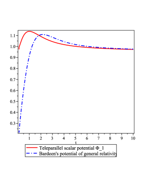
Figure 1: Scalar teleparallel perturbation potentials $\Phi_{1}$ and its general relativistic counterparts for chaotic potential $V(\phi)=\frac{1}{2}m^{2}\phi^{2}$ . The plots are for the wavenumber value $k=\frac{1}{1000}\,hMpc^{-1}$. The time axis is in Gigayears

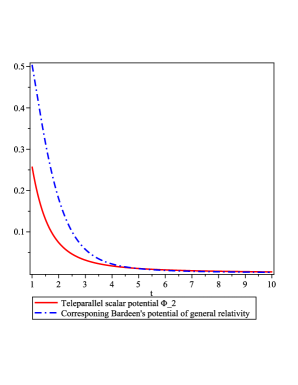
Figure 2: Scalar teleparallel perturbation potentials $\Phi_{2}$ and its general relativistic counterparts for the chaotic potential $V(\phi)=\frac{1}{2}m^{2}\phi^{2}$ . The plots are for the wavenumber value $k=\frac{1}{1000}\,hMpc^{-1}$. The time axis is in Gigayears

Here we are concerned with a case where there is no anisotropic stress and no momentum perturbation. In this case we can solve equations (39) and (40) together to find the two invariant perturbation potentials $\Phi_{1}$ and $\Phi_{2}$ and then use one of the constraint equations (41) or (42) to find the gauge invariant density perturbation $\Phi_{\rho}$. The numerical analysis is done for three types of cosmologically interesting potentials.
$\bullet$ Chaotic potential: Figures (1) and (2) show the time evolution of geometric potentials $\Phi_{1}$ and $\Phi_{2}$ versus the cosmic time when the scalar field potential is assumed to be of the chaotic type i.e. $V(\phi)=\frac{1}{2}m^{2}\phi^{2}$. For comparison, we also plotted the corresponding potentials deriving from the theory of general relativity. As can be seen from the figures, the results are different at early times (high energies) but coincide at late times.
$\bullet$ Exponential potential: Figures (3) and (4) show the time evolution of geometric potentials $\Phi_{1}$ and $\Phi_{2}$ versus the cosmic time for potential in the form of $V(\phi)=V_{0}e^{-\lambda\phi}$. Here again the results show the same trend, however the potentials coincide at at a slightly later time than the previous case.
$\bullet$ Power law potential: Figures (5) and (6) show the results for potential in the form of $V(\phi)=\lambda\phi^{4}$. In this case the potentials for teleparallel and general relativity theories coincide at an earlier time than the first case.

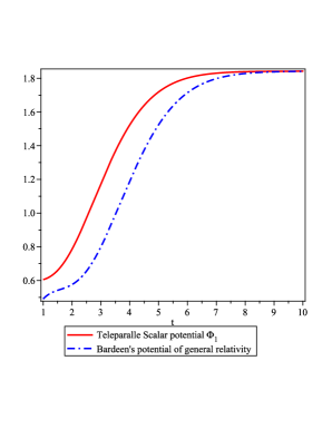
Figure 3: Scalar teleparallel perturbation potentials $\Phi_{1}$ and its general relativistic counterparts for exponential potential $V(\phi)=V_{0}e^{-\lambda\phi}$ . The plots are for the same value of wavenumber $k$ as in previous figures

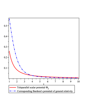
Figure 4: Scalar teleparallel perturbation potentials $\Phi_{2}$ and its general relativistic counterparts for exponential potential $V(\phi)=V_{0}e^{-\lambda\phi}$ and the same value of the wavenumber $k$ as before .

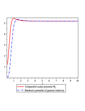
Figure 5: Scalar teleparallel perturbation potentials $\Phi_{1}$ and its general relativistic counterparts for potential $V(\phi)=\lambda\phi^{4}$. Other parameters are the same as previous figures.

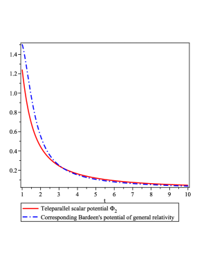
Figure 6: Scalar teleparallel perturbation potentials $\Phi_{2}$ and its general relativistic counterparts for potential $V(\phi)=\lambda\phi^{4}$ .

8 Conclusion

The theory of TEGR is obtained from gauging the translational part of the Lorentz group and after applying some restrictions on the PGT Lagrangian will turn into a theory which is also invariant under local Lorentz transformation. These properties has led the theory to be dynamically equivalent to GR while they still have some conceptual differences. This equivalence has led to a reluctance in studying many physical issues in the context of TEGR but the special geometric structure of this theory has some interesting features to study. In the context of cosmological perturbations the results of directly perturbing FRW vierbeins, are found to be different from the results obtained from perturbing FRW metric in general relativity. This difference stems from different transformational properties of tetrad and metric under a gauge transformation. These transformational properties are obtained by considering Lie derivative of the dynamical variables of the theory. In a teleparallel setup, one may use the gauge covariant Lie derivative which is not equivalent to the ordinary Lie derivative used in general relativity. Another difference comes from the fact that tetrad perturbations only have scalar and vector modes in the coordinate frame. As a result, the tensorial part will manifest itself as a combination of the vector perturbations modes in the metric. Studying cosmological issues in this context and comparing the results by observational data, concerning all the points mentioned above, seem to be interesting. In this paper also the gauge invariant perturbed field equations have been found and by means of gauge potentials. The formalism developed here can be readily extended for use in $f(T)$ theories of gravity. However in the $f(T$, case extreme care is needed in defining the gauge invariant potentials as some of these models show violations of local Lorentz invariance. In that case a gauge invariant potential should remain unchanged under both a general coordinate transformation and a local lorentz rotation of the frame.

Appendix A

In this appendix we present the non-zero components of the torsion and contorsion tensors, superpotential and the torsion scalar of the perturbed tetrad (19)

Metric and inverse metric

$$g_{00}=-a^{2}(1+2A)\quad,\quad g_{0\alpha}=a^{2}(B_{\alpha}-C_{\alpha})\quad,\quad g_{\alpha\beta}=a^{2}(\delta_{\alpha\beta}+D_{\alpha\beta})\quad,\quad$$

$$g^{00}=-\frac{1}{a^{2}}(1-2A)\quad,\quad g^{0\alpha}=\frac{1}{a^{2}}(C^{\alpha}-B^{\alpha})\quad\quad,\quad\quad g^{\alpha\beta}=\frac{1}{a^{2}}(\delta^{\alpha\beta}-D^{\alpha\beta})$$

Weitzenböck connection coefficients

$$\Gamma_{~{}~{}\alpha\beta}^{\gamma}=\partial_{\beta}D_{~{}~{}\alpha}^{\gamma}\quad,\quad\Gamma_{~{}~{}0\beta}^{\gamma}=\partial_{\beta}B^{\gamma}\quad,\quad\Gamma_{~{}~{}\alpha 0}^{\gamma}=h\delta^{\gamma}_{\alpha}+D_{~{}~{}\alpha}^{{}^{\prime}\gamma}\quad,\quad\Gamma_{~{}~{}00}^{\gamma}=B^{{}^{\prime}\gamma}$$

$$\Gamma_{~{}~{}\alpha\beta}^{0}=\partial_{\beta}C_{\alpha}\quad,\quad\Gamma_{~{}~{}0\beta}^{0}=\partial_{\beta}A\quad,\quad\Gamma_{~{}~{}\alpha 0}^{0}=C^{\prime}_{\alpha}\quad,\quad\Gamma_{~{}~{}00}^{0}=h+A^{\prime}$$

Torsion

$$T_{0\alpha}^{0}=C^{\prime}_{\alpha}-\partial_{\alpha}A\quad,\quad T_{\alpha\beta}^{0}=2\partial_{\,\,[\alpha}C_{\beta]}$$

$$T_{\beta 0}^{\alpha}=h\delta_{\beta}^{\alpha}-\partial_{\beta}B^{\alpha}+D_{\beta}^{{}^{\prime}\alpha}\quad,\quad T_{\beta\gamma}^{\alpha}=2\partial_{\,[\beta}D_{\gamma]}^{\alpha}$$

Contorsion

$$K_{~{}~{}0}^{\alpha 0}=\frac{-1}{a^{2}}\Big{[}C^{{}^{\prime}\alpha}-\partial^{\alpha}A\Big{]}$$

$$K_{~{}~{}0}^{\alpha\beta}=\frac{1}{a^{2}}\Big{[}2D^{{}^{\prime}[\alpha\beta]}-\partial^{[\beta}B^{\alpha]}-\partial^{[\alpha}C^{\beta]}\Big{]}$$

$$K_{~{}~{}\beta}^{\alpha 0}=\frac{1}{a^{2}}\Big{[}-\partial_{(\beta}B^{\alpha)}+\partial^{[\alpha}C_{\beta]}+h(1-2A)\delta_{\beta}^{\alpha}-D_{~{}~{}\beta}^{{}^{\prime}\alpha}\Big{]}$$

$$K_{~{}~{}\gamma}^{\alpha\beta}=\frac{-1}{a^{2}}\Big{[}\partial^{[\beta}D_{~{}~{}\gamma]}^{\alpha}-\partial^{[\alpha}D_{~{}~{}\gamma]}^{\beta}-\partial^{[\alpha}D_{\gamma}^{~{}~{}\beta]}$$

$$+2h(\delta^{~{}[\alpha}_{\gamma}C^{\beta]}-\delta^{~{}[\alpha}_{\gamma}B^{\beta]})\Big{]}$$

Superpotential

$$S^{~{}~{}\alpha\beta}_{\gamma}=\frac{1}{2a^{2}}\Big{[}-\partial^{[\beta}D_{~{}~{}\gamma]}^{\alpha}+\partial^{[\alpha}D_{~{}~{}\gamma]}^{\beta}+2\delta^{\alpha}_{\gamma}\partial^{[\beta}D_{~{}~{}\eta]}^{\eta}$$

$$-2\delta^{\beta}_{\gamma}\partial^{[\alpha}D_{~{}~{}\eta]}^{\eta}-2(\delta^{~{}[\alpha}_{\gamma}C^{{}^{\prime}\beta]}-\delta^{~{}[\alpha}_{\gamma}\partial^{\beta]}A)$$

$$~{}~{}~{}~{}~{}+2h(\delta^{~{}[\alpha}_{\gamma}C^{\beta]}-\delta^{~{}[\alpha}_{\gamma}B^{\beta]})\Big{]}$$

$$S^{~{}~{}\alpha 0}_{\gamma}=\frac{1}{2a^{2}}\Big{[}-\partial_{(\gamma}B^{\alpha)}+\delta^{\alpha}_{\gamma}\partial_{\eta}B^{\eta}+\partial^{[\alpha}C_{\gamma]}+D_{~{}~{}~{}\gamma)}^{{}^{\prime}(\alpha}-\delta^{\alpha}_{\gamma}D_{~{}~{}\eta}^{{}^{\prime}\eta}$$

$$-2\frac{h}{a^{2}}\delta^{\alpha}_{\gamma}(1-2A)\Big{]}$$

$$S^{~{}~{}\alpha\beta}_{0}=\frac{1}{2a^{2}}\Big{[}D^{{}^{\prime}[\alpha\beta]}-\partial^{[\beta}B^{\alpha]}-\partial^{[\alpha}C^{\beta]}\Big{]}$$

$$S^{~{}~{}\alpha 0}_{0}=-\frac{1}{a^{2}}\partial^{[\alpha}D_{~{}~{}\eta]}^{\eta}-\frac{3h}{a^{2}}(C^{\alpha}-B^{\alpha})$$

Torsion scalar

$$T=-6\frac{h}{a^{2}}\partial_{\eta}B^{\eta}-\frac{h}{a^{2}}\partial^{[\eta}C_{\eta]}+6\frac{h^{2}}{a^{4}}D_{~{}~{}\eta}^{{}^{\prime}\eta}+6\frac{h^{2}}{a^{4}}(1-2A)$$

References

- [1] J.M. Bardeen, Phys. Rev. D22, 1882 (1980); J.M. Bardeen, P. J. Steinhardt and M. S. Turner, Phys. Rev. D28, 679 (1983).
- [2] H. Kodama and M. Sasaki, Frog. Theor. Phys. Suppl. No. 78 (1984) 1.
- [3] V.F. Mukhanov, H.A. Feldman and R.H. Brandenberger, Phys. Rept. 215, 203 (1992).
- [4] R. Durrer, Astron. Astrophys. 208 (1989) 1.
- [5] A. Riotto, arXiv:hep-ph/0210162
- [6] A. Einstein, Math. Annal. 102, 685 (1930). For an english translation, see A. Unzicker and T. Case, [physics/0503046v1].
- [7] F. W. Hehl and Y. N. Obukhov, Annales Fond.Broglie. 32 (2007) 157-194 arXiv:gr-qc/0711.1535
- [8] K. Hayashi and T. Shirafuji, Phys. Rev. D 19, 3524 (1979); K. Hayashi and T. Shirafuji, Phys. Rev. D 24, 3312 (1981).
- [9] R. Aldrovandi and J. G. Pereira, An Introduction to Teleparallel Gravity, Instituto de Fisica Teorica, UNSEP, Sao Paulo, (2010).
- [10] R. Aldrovandi, J. G. Pereira, Teleparallel Gravity An Introduction, Fundamental Theories of physics, Springer (2013)
- [11] T. P. Sotiriou, B. Li and J. D. Barrow, Phys .Rev. D 83 , 104030 (2011)
- [12] R. Ferraro and F. Fiorini, Phys. Rev. D 75, 084031 (2007); N. Tamanini and C. G. Boehmer, Phys. Rev. D 86 , 044009 (2012); Y. -P. Wu, C. -Q. Geng, [arXiv:1110.3099]; M. E. Rodrigues, M. J. S. Houndjo, D. Saez-Gomez, F. Rahaman, Phys. Rev. D 86, 104059 (2012); K. Bamba, R. Myrzakulov, S. Nojiri and S. D. Odintsov, Phys. Rev. D 85, 104036 (2012); K. Bamba, S. Capozziello, S. Nojiri, S. D. Odintsov [arXiv:1205.3421].
- [13] S. Nojiri and S. D. Odintsov, Phys. Rept. 505, 59-144,(2011), arXiv:1011.0544 [gr-qc]
- [14] S. Nojiri and S. D. Odintsov, Int.J.Geom.Meth.Mod.Phys.4,115-146 (2007), [hep-th/0601213]
- [15] M. Blagojevic, Gravitation and Gauge Symmetries (IoP Publishing, Bristol, 2002); M. Blagojevic, Three lectures on Poincare gauge theory, SFIN A 1, 147 172 (2003) [gr-qc/ 0302040]; M. Blagojevic and F.W. Hehl (eds.), GAUGE THEORIES OF GRAVITATION A Reader with Commentaries Foreword by T.W.B. Kibble, FRS Imperial College Press, London, February 2013
- [16] F. W. Hehl and B. Mashhoon, Phys. Lett. B 673, 279 (2009) [arXiv: 0812.1059 [gr-qc]]; F. W. Hehl and B. Mashhoon, Phys. Rev. D 79, 064028 (2009) [arXiv: 0902.0560 [gr-qc]].
- [17] R. Weitzenböck, Invariance Theorie, Nordhoff, Groningen, 1923.
- [18] J.M. Stewart, Class. Quant. Grav. 7, 1169 (1990).
- [19] J. M. Stewart and M. Walker, Proc. R. Soc. A (1974) 341 49-74
- [20] F. W. Hehl, J. D. McCrea, E. W. Mielke, and Y. Ne eman, Metric affine gauge theory of gravity: Field equations, Noether identities, world spinors, and breaking of dilation invariance, Phys. Rept. 258, 1 171 (1995).
- [21] J.M. Nester: Gravity, torsion and gauge theory, in: Introduction to Kaluza-Klein theories, H.C. Lee, ed. (World Scientific, Singapore 1984) pp. 83-l 15.
- [22] J.M. Nester: Lectures on gravitational gauge theory, Hsinchu School on Gravitation, Relativity and Cosmology, Hsinchu, Taiwan, I l-13 Nov. 1989.