Stability and Equilibrium Analysis of Laneless Traffic with Local Control Laws

Abstract

In this paper, a new model for traffic on roads with multiple lanes is developed, where the vehicles do not adhere to a lane discipline. Assuming identical vehicles, the dynamics is split along two independent directions—the $Y$-axis representing the direction of motion and the $X$-axis representing the lateral or the direction perpendicular to the direction of motion. Different influence graphs are used to model the interaction between the vehicles in these two directions. The instantaneous accelerations of each car, in both $X$ and $Y$ directions, are functions of the measurements from the neighbouring cars according to these influence graphs. The stability and equilibrium spacings of the car formation is analyzed for usual traffic situations such as steady flow, obstacles, lane changing and rogue drivers arbitrarily changing positions inside the formation. Conditions are derived under which the formation maintains stability and the desired intercar spacing for each of these traffic events. Simulations for some of these scenarios are included.

I Introduction

This paper is motivated by the desire to develop models to analyze traffic when the roads are wide and the lanes are blurred. Such traffic behavior is not uncommon in many roads in India where, to misquote J K Galbraith, a ‘functioning anarchy’ prevails. We develop a stylized model to describe the local interaction among the vehicles on such roads and use this microscopic description to characterize the emerging macroscopic behaviour. In effect, we consider a multilane system except that we assume that there is no strict demarcation of lanes and that vehicles are affected by those in a ‘cone’ rather than by the vehicle right ahead. On such roads, multiple cars drive abreast but do not adhere to lane discipline. Toward this we adapt the single lane model of [6] to develop our multilane model. Specifically, a directed graph is used to model the influence on the acceleration of a vehicle by others in its neighbourhood, i.e., those that are in its cone. We seek an equilibrium analysis of the dynamical system model that we develop. Our notion of stability refers to the condition that all cars attain the same velocity as the leader. Since this is a car following model, we also have the notion of levels and the analysis will also obtain conditions such that cars in one ‘level’ maintain a fixed spacing from cars in the next ‘level.’ Our analysis will primarily use the Laplacian of the directed graph that models the influences, which in turn will allow us to dissolve the lanes, so to say. The influence graph can also be a weighted graph to enable us to model the relative degrees of the influences.

Models for vehicular systems have been widely studied both from a microscopic [5] [7] as well as from a macroscopic [9] [22] perspective. Various forms of stability such as input-to-state [30], string stability [29] and mesh stability have been considered. Mesh stability ensures damping of perturbations in vehicle formations, as they move away from the source [27][21][28]. Various applications are studied namely obstacle avoidance in [20] and lane changing in [14] [8]. In [11] multilane model for vehicular traffic is considered and a fluid model is developed. Unlike string or mesh stability theories, where the main concern is magnification of disturbances down infinite chains of cars, in this paper, we study finite number of cars. While it is relatively easy to show stability properties in this case, we are concerned primarily about equilibrium spacing between the cars. We show that it is possible, with purely distributed control laws, to achieve and maintain desired spacing, even in an ad-hoc laneless traffic situation under a variety of common traffic conditions and disturbances.

The results presented here, as well as the tools used to derive those results, are heavily dependent on the theory of consensus in multiagent systems (see e.g [4] [10][19][24] and the references therein). While [26] has studied vehicle consensus, [23][17] derived stability conditions for time varying topologies. Most of our analysis depend on these recently developed theories and particularly on [25], where arbitrary vehicle formations (not necessarily unidirectional as in roadways) have been studied. We specialize these results for ad-hoc laneless road traffic, and in the process derive distributed control laws that preserve inter-vehicle spacing and stability under time-varying formations, switched influence graphs and impulse changes in driving objectives. While these properties are hard to derive for general types of motion, it becomes relatively simple here due to typical uni/bi-directional constrained motion possible on roadways.

The rest of the paper is organized as follows. In Section II we set up the notation and our assumptions on the models for the $X$ and the $Y$ directions. We then describe the control laws that are used by the vehicles for each of $X$ and $Y$ directions. In Section III, we analyze the dynamics of motion in the $Y$ direction and obtain a stability criterion. We also characterize the influence graph. A similar analysis is carried out for the $X$ direction in Section IV. In Section V we present the analysis when the influence graph varies with time. In Section VI we analyze the effects of impulses on the stability of the formation. Finally, in Section VII we present some simulation results.

II Traffic Model and Control Laws

As discussed in the introduction, we are interested in analyzing the motion of a finite number of cars along roads which has no lane demarcations. In other words, cars can, in principle, occupy arbitrary positions with respect to other cars as long as they do not collide with each other or with the side of the road. However, all the cars want to travel along the road in one direction and would also like to keep safe a distance from all its neighbours based on visual feedback about the position and velocity of the neighbouring cars. We name the direction of travel along the road as the $Y$-axis and the direction perpendicular to the road as the $X$-axis. Though in reality, a car’s ability to maneuver in these two directions is coupled, for simplicity we assume that the dynamics of each car along these two directions are independent. Moreover, the control laws for each of these directions consider a different set of influencing neighbours. This later assumption is realistic since a driver typically looks to the side before moving sideways, while he considers only the cars roughly in front of him for normal forward motion. In effect, the influence graphs for the $X$ and $Y$ directions are different in our calculations. In addition, we also assume, again for simplicity, that the cars in the formation are identical. We state the various modeling assumptions along these two directions after a brief description of graph theoretic notation.

II-A Notation

The sets of naturals, reals, positive reals and real $n$ tuples are denoted by $\mathbb{N}$, $\mathbb{R}$, $\mathbb{R}^{+}$ and $\mathbb{R}^{n}$. An undirected graph $\mathcal{G}=(\mathcal{V},\mathcal{E},w)$ is a finite set of nodes $\mathcal{V}$ connected by a set of edges $\mathcal{E}\subset\mathcal{V}\times\mathcal{V}$ along with a function $w:\mathcal{E}\rightarrow\mathbb{R}^{+}$. When two nodes $a_{i}\in\mathcal{V}$ and $a_{j}\in\mathcal{V}$ are connected to each other the graph $\mathcal{G}$ said to have an edge between $a_{i}$ and $a_{j}$, denoted by $(a_{i},a_{j})\in\mathcal{E}$. A graph is said to be connected when there exists a path between any two nodes. A spanning tree is a connected graph $\mathcal{G}_{tree}=(\mathcal{V}_{tree},\mathcal{E}_{tree})$ having no cycles in the graph. If the edges of a graph $\vec{\mathcal{G}}=(\mathcal{V},\vec{\mathcal{E}})$ are directed i.e. $(a_{i},a_{j})\in\vec{\mathcal{E}}\nRightarrow(a_{j},a_{i})\in\vec{\mathcal{E}}$, the graph is called a directed graph (or digraph). A rooted directed tree is a digraph such that there exists a node (called root) and a directed path from that node to all other nodes in the digraph. A digraph $\vec{\mathcal{G}}$ is said to contain a directed spanning tree, if there exists a rooted directed tree $\vec{\mathcal{G}}_{tree}=(\mathcal{V}_{tree},\vec{\mathcal{E}}_{tree})$ such that $\mathcal{V}_{tree}=\mathcal{V}$ and $\vec{\mathcal{E}}_{tree}\subseteq\vec{\mathcal{E}}$. We define the Laplacian (${L}$) for a directed graph with weights $w_{ij}$ as follows: $\ell_{ij}:=-1\quad\mbox{if}\quad j\rightarrow i\quad\mbox{and}\quad\ell_{ii}=\sum_{j=1}^{n}w_{ij}:=\mbox{indegree}$.

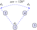
(a) $Y$ direction motion: car $3$ is
not seen by car $1$

(b) $X$ direction motion: black lines indicate the underlying graph

Figure 1: Different influence graphs for $X$ and $Y$ direction depending on the angle of view ($aov$) of the car

II-B Assumptions for $Y$-direction

A1) For determining the influence in $Y$ direction we consider each driver to have a fixed viewing angle ($aov$) of $120$° and a car must be within this viewing angle to influence the driver. This forms the conical section $d_{1}d_{2}d_{3}$ as shown in Figure 1(a). In this figure cars 2 and 4 lie within the conical section $d_{1}d_{2}d_{3}$ formed by car 1 and hence can influence car 1. Car 3 being outside the cone cannot influence car 1.

A2) We assume that the convoy follows a fictitious leader in the direction of travel. As discussed later, the role of the leader node is to set a desired velocity for our formation. This fictitious leader can be considered as a mathematical representation of velocity limiting rules, regulations or driver experience in practice. In Figure 3(a) node $0$ is the leader.

A3) The influence graph for $Y$ axis is assumed to have a directed spanning tree with node $0$ as the root. This assumption is equivalent to connectedness of the influence graph in this framework.

A4) Cars with same number of hops from the leader node are referred to as being in the same ‘level’. In Figure 3(a) cars $1,2,$ and $3$ belong to level one.

A5) We assume that influence of any car extends up to a maximum of one level for ease of exposition. This is elaborated on in later sections.

A6) The convention used for numbering cars in the graph is as follows: (i) Cars are numbered according to their levels with cars in higher levels having higher numbers. (ii) Cars in the same level are numbered from left to right with left most car being the highest number in that level.

A7) We assume that each node can choose the distribution of weights on its incoming links. This is related to the driver’s discretion about relative importance of the various cars in front of him.

II-C Distributed Control Laws for $Y$-direction

Consider a convoy of cars represented by influence graphs as shown in Figure 3(a) along $Y$ direction, where node $0$ is assumed to move at an arbitrary velocity $v_{0}$. We assume that in the direction of travel, the last car has the lowest nonnegative $y$ coordinate: car $9$ will have the lowest nonnegative $y$ coordinate and car $0$ has the highest $y$ coordinate in Figure 3(a). Let the velocity and position of car $i$ for motion in $Y$-direction be denoted by $v_{yi}$ and $y_{i}$. The proposed control law model for car $i$ in $Y$ direction is a modified version of single lane car following model of [6] and is as follows,

$$\dot{y_{i}} =v_{yi}$$

$$\dot{v}_{yi} :=\sum_{j=\mathcal{N}(i)}b(w_{ij}v_{yj}-w_{ii}v_{yi})+k(w_{ii}y_{j}-w_{ii}y_{i}-g_{y})$$ (1)

Here $\mathcal{N}(i)$ represents the neighbour set of car $i$, $w_{ij}$ is the weight given to link connecting node $j\to i\ \forall\ j\neq i$, $w_{ii}=\sum_{j=1}^{n}w_{ij}=:W$, $b$ and $k$ are constants, and parameter $g_{y}$ is a tuning parameter used to adjust the equilibrium distance between cars in consecutive levels. Consider an $n$ car formation with node $0$ as leader moving along the road. Let $y\in\mathbb{R}^{n+1}$ represent the $y$ coordinates or absolute position of $n+1$ cars. $v_{y}\in\mathbb{R}^{n+1}$ represent the velocities of the cars.

A graph $\mathcal{G}=(\mathrm{V},\mathcal{E},w)$ having a node set $\mathrm{V}$ and an edge set $\mathcal{E}$ is used to denote the influence diagram between various cars as per A1. Each node in the graph represents a vehicle (agent). The directed edges are introduced as follows: If vehicle $j$ can be sensed by vehicle $i$ ($i\neq j$), then an edge from $j$ to $i$ exists with weight $w_{ij}$ and is denoted by $j\rightarrow i$. Then the control law in (II-C) can be written as follows:

$$\begin{bmatrix}\dot{y}\\ \dot{v_{y}}\end{bmatrix}=\begin{bmatrix}\mathrm{0}&\mathrm{I}\\ -k\ {L^{y}}&-b\ {L^{y}}\end{bmatrix}\begin{bmatrix}{y}\\ {v_{y}}\end{bmatrix}-kg_{y}\begin{bmatrix}\mathbf{0}\\ \mathbf{1}\end{bmatrix}$$ (2)

where $\mathbf{1}\in\mathbb{R}^{n},\ \mathbf{0}\in\mathbb{R}^{n+2},$ ${L^{y}}$ denotes the Laplacian of the directed weighted influence graph.

II-D Assumptions for $X$-direction

B1) For motion in $X$-direction the angle of viewing extends to $180$°. This is reasonable since a driver would usually look sideways before making a sideways deviation. In Figure 1(b) car $1$ is influenced by cars $2,3,$ and $4$.

B2) For horizontal motion, the boundary of the road needs to be incorporated into the model. This is achieved by assuming some fictitious cars are moving along the boundary of the road at each ‘level’. Levels are still defined using the $Y$-direction influence graph and hops from the pseudo $0$-node. In Figure 3(b) cars $1,5,9$, enclosed by the red block, represent the boundary of the road. These nodes have same dynamics as the regular cars but move under slightly specialized laws: (i) these nodes have no horizontal velocity (ii) they continue to have the same $y$-coordinate and the same $y$ velocity as the leftmost car in the corresponding level (iii) boundary nodes are influenced only by other boundary nodes from the levels directly above them. In Figure 3(b) car $5$ is assumed to be influenced only by car $1$ and car $9$ only by car $5$. Although the more general case of roads having boundaries on both sides can be incorporated in the model, here we analyze the system with boundary on one side of the road for simplicity of exposition.

B3) For $X$ axis motion node $1$ is assumed to play the role of the leader node as shown in Figure 3(b). This again sets the $x$ velocity of the formation.

B4) The influence graph for $X$ direction is assumed to have a directed spanning tree with node $1$ as root.

II-E Distributed Control Laws for $X$-direction

Let the velocity and position for car $i$ be denoted by $v_{xi}$ and $x_{i}$. The proposed control law for car $i$ in $X$-direction is

$$\dot{x_{i}}=v_{xi}$$

$$\dot{v}{}_{xi}:=\sum_{j=\mathcal{N}(i)}b_{x}(w_{ij}v_{xj}-w_{ii}v_{x(i)})+k_{x}(w_{ij}x_{j}-w_{ii}x_{i}-z_{i}g_{x})$$ (3)

where $\mathcal{N}(i)$ represents the neighbour set of car $i$, $w_{ij}$ is the weight given to link connecting node $j\to i\ \forall\ j\neq i$, $w_{ii}=\sum_{j=1}^{n}w_{ij}=:W$, $b_{x}$ and $k_{x}$ are constants, and parameter $g_{x}$ is tuned for desired equilibrium distance between cars in the same level. This law differs from the $Y$-axis law in that it requires some extra parameters $z_{i}$’s to ensure the desired inter-car spacing. The $X$ axis motion of $n$ cars in the formation is described below. Let $x\in\mathbb{R}^{n}$ denotes the coordinates and $v_{x}\in\mathbb{R}^{n}$ represent the velocities in the $X$ direction. The control law in (II-E) is as follows:

$$\begin{bmatrix}\dot{x}\\ \dot{v}_{x}\end{bmatrix}=\begin{bmatrix}\mathit{0}&\mathrm{I}\\ -k_{x}\ {L^{x}}&-b_{x}\ {L^{x}}\end{bmatrix}\begin{bmatrix}{x}\\ {v_{x}}\end{bmatrix}+kg_{x}\begin{bmatrix}\mathbf{0}\\ C\end{bmatrix}$$ (4)

where $\mathbf{1}\in\mathbb{R}^{n}$ and $\mathbf{0}\in\mathbb{R}^{n}\mbox{ and }\mathit{0}\in\mathbb{R}^{n\times n},\ C\in\mathbb{R}^{n}$.

$$C:=\begin{bmatrix}0&z_{2}\ \ldots\ z_{k}&0&z_{k+1}\ldots&0&\ldots\ z_{n}\end{bmatrix}$$

where the nonzero $z_{1},\ z_{2},\ldots\ z_{n}$ are constants locally computed by each car to ensure a spacing of $g_{x}$ between cars in the same level. The ${L^{x}}$ denotes the directed weighted Laplacian of the $X$-axis influence graph. The dependence of $z_{i}$ and $g_{x}$ is elaborated on in later sections.

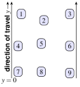
Figure 2: The convoy of cars for which the influence graphs are represented below

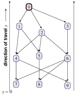
(a) Information flow along
$Y$ axis

(b) Information flow along
$X$ axis

Figure 3: Figures show the influence graphs for both directions

III Analysis of $Y$-dynamics

In this section we give conditions under which control law (2) gives the desired spacing with unidirectional communication for $Y$ axis motion. We rewrite (2) with the position ($y_{0}(t)$) and velocity ($v_{0}(t)$) of leader node $0$ as external inputs:

$$\begin{bmatrix}\dot{y}\\ \dot{v_{y}}\end{bmatrix}=\begin{bmatrix}\mathrm{0}&\mathrm{I}\\ -k\ \tilde{{L}}^{y}&-b\ \tilde{{L}}^{y}\end{bmatrix}\begin{bmatrix}{y}\\ {v_{y}}\end{bmatrix}-kg_{y}\begin{bmatrix}\mathbf{0}\\ \mathbf{1}\end{bmatrix}+\begin{bmatrix}\mathbf{0}\\ B^{y}\end{bmatrix}\begin{bmatrix}bv_{0}\\ ky_{0}\end{bmatrix}$$ (5)

where $B^{y}\in\mathbb{R}^{n\times 2}$, $y,\;v_{y}\in\mathbb{R}^{n}$. $\tilde{{L}}^{y}$ is the reduced Laplacian obtained from ${L^{y}}$ after removing the row and column corresponding to node $0$. $B^{y}$ contains the columns from ${L^{y}}$ which denote the links between the leader node $0$ and the remaining cars in the formation. For Figure 3(a), assuming unit weights, $B^{y}$ is given by,

$$B^{y}=\begin{bmatrix}1&1&1&0&0\ldots 0\\ 1&1&1&0&0\ldots 0\end{bmatrix}^{T}$$ (6)

In (6), the $1$’s in $B^{y}$ represents information flow from node $0$ to cars $1,2,3$. We give our first main result for $Y$ direction motion of a convoy having node $0$ as leader. Let

$$\hat{y}:=\begin{bmatrix}y&v_{y}\end{bmatrix}^{T}\quad\mbox{ and }\quad\Gamma^{y}:=\begin{bmatrix}\mathrm{0}&\mathrm{I}\\ -k\ \tilde{{L}}^{y}&-b\ \tilde{{L}}^{y}\end{bmatrix}$$ (7)

Theorem III.1

Consider a weighted directed graph such that the total weight ($W$) across all incoming edges is the same for each node. Then the autonomous system $\dot{\hat{y}}=\Gamma^{y}\hat{y}$ achieves an asymptotically stable equilibrium point at the origin ($0\in\mathbb{R}^{2n}$). Moreover if the leader velocity $v_{y0}$ is constant, then:

1. $v_{yi}\rightarrow v_{y0}\ \mbox{as }t\rightarrow\infty\;\forall\ i\in\{1,\ldots n\}$

2. $|y_{i}(t)-y_{j}(t)|\rightarrow 0$ as $t\rightarrow\infty$ for all $i,j$ in the same level.

3. At equilibrium, the relative spacing between cars in two consecutive levels is $g_{y}/W$.

Before proving the theorems we note that the weighted Laplacian has a zero row corresponding to the phantom leader, has non-negative real eigenvalues and $0$ is a simple eigenvalue, with $\begin{bmatrix}1&0&\ldots&0\end{bmatrix}$ as its left eigenvector, and the Laplacian right nullspace consists of the vector $[1\ 1\ \ldots\ 1]^{T}$. Additionally the following result holds.

Lemma III.2

Under the numbering scheme in Assumption II-B, the influence graph has no cycles and the Laplacian (${L^{y}}$) has a lower triangular structure. Moreover, the diagonal entries of ${L^{y}}$ will be same for all rows excluding the rows representing level one and node $0$.

Proof of Theorem III.1:

We first analyze the asymptotic stability of the autonomous part of the system in (5). From [25] we get $Re(\lambda_{i}(\Gamma))<0\ \forall\ i,\ \forall\ b,\;k>0,$ if $\lambda_{j}(-\tilde{{L}}^{y})<0\ \ \forall\ j$ and $\lambda_{j}(\tilde{{L}}^{y})\in\mathbb{R}\ \forall\ j$, where $Re(.)$ denotes the real part. The equilibrium point for the autonomous part of the system in (5) is $v_{y}=0$ and $-\tilde{{L}}^{y}y=g_{y}$.

Next we analyze the system in (5) at equilibrium with fixed velocity $v_{0}$ of node $0$ as input. The required spacing can be computed from.

$$-{L^{y}}y=g_{y}\begin{bmatrix}0\\ \mathbf{1}\end{bmatrix}$$ (8)

where $\mathbf{1}\in\mathbb{R}^{n}$ for $n+1$ nodes. Now we use induction. Cars in the first level will have one link connecting to the node $0$ by A2. For any car $i$ in the first level from (8) we get, $y_{0}=y_{i}+g_{y}/W$. This will ensure that all cars in the first level have the same $y$ coordinate.

Consider some car $i$ in level $\mathcal{I}$. Let cars in the level above be denoted by $j_{1},j_{2},\ldots,j_{n}$. Let $y$ coordinates of the cars $j_{1},\ldots,j_{n}$ be same. Let the weights on the links from car $j_{1}$ to car $i$ be denoted by $w_{ij_{1}}$ and so on. The $i^{th}$ row in (8) can be expressed as follows: $w_{ij_{1}}y_{j_{1}}+w_{ij_{2}}y_{j_{2}}\ldots+w_{ij_{n}}y_{j_{n}}=g_{y}+Wy_{i}.$ From induction hypothesis, $y_{j}=y_{i}+g_{y}/W$. This completes the proof. $\Box$

Clearly, for unweighted influence graphs, the conditions for Theorem III.1 reduces to each car having the same indegree (say $M$), thereby guaranteeing the relative spacing between two consecutive levels to be $g_{y}/M$.

IV Analysis of $X$-dynamics

In this section we analyze the vehicle motions in $X$-direction under the assumptions stated in Section II-D. The analysis, while being similar to the $Y$-dynamics, differs in some crucial features. One of the main differences arise since the influence graph can be bidirectional (see Figure 3(b)): in other words, two drivers can simultaneously look towards each other and decide on their $X$-control. Secondly, recall that the $X$-velocities of the pseudo (road boundary) cars (e.g. cars 1, 5, 9) are zero by assumption (e.g. $v_{x1}=v_{x5}=v_{x9}=0$), and hence their $X$-positions are always constant ($x_{1}=x_{5}=x_{9}=$ constant). Hence when we rewrite (4) with node $1$ velocity and position as external input,

$$\begin{bmatrix}\dot{x}\\ \dot{v}_{x}\end{bmatrix}=\begin{bmatrix}\mathit{0}&\mathrm{I}\\ -k_{x}\ \tilde{{L}}^{x}&-b_{x}\ \tilde{{L}}^{x}\end{bmatrix}\begin{bmatrix}{x}\\ {v_{x}}\end{bmatrix}+k_{x}g_{x}\begin{bmatrix}\mathbf{0}\\ C\end{bmatrix}+\begin{bmatrix}\mathbf{0}\\ B^{x}\end{bmatrix}\begin{bmatrix}0\\ k_{x}x_{1}\end{bmatrix}$$ (9)

where $x,v_{x}\in\mathbb{R}^{n-1}$, $B^{x}$ contains the columns from ${L^{x}}$ which denote the links between the leader node 1 and the remaining cars in the formation. We assume that every car wants to position themselves at a distance $g_{x}$ from both adjoining cars in the same ’level’. Let,

$$\hat{x}:=\begin{bmatrix}x&v_{x}\end{bmatrix}^{T}\quad\mbox{and}\quad\Gamma^{x}:=\begin{bmatrix}\mathrm{0}&\mathrm{I}\\ -k_{x}\ \tilde{{L}}^{x}&-b_{x}\ \tilde{{L}}^{x}\end{bmatrix}$$ (10)

Theorem IV.1

Under the above assumptions, there exists $b$, $k$ such that the autonomous system $\dot{\hat{x}}=\Gamma^{x}\hat{x}$ asymptotically achieves equilibrium at the origin ($0\in\mathbb{R}^{2n})$. Moreover,

1. $v_{xi}(t)\rightarrow 0\ \mbox{as }t\rightarrow\infty\;\forall\ i\in\{1,\ldots,n\}$.

2. There exist $C$ such that $|x_{i}-x_{i+1}|\rightarrow g_{x}$ as $t\rightarrow\infty$ for $i,i+1$ in same level.

3. The $C$ achieving (2) can be computed locally.

For obtaining a spacing of $g_{x}$ between cars in the same level, we impose the additional constraints for cars $i$ and $i+1$ in the same level (denoted by $\mathcal{I}$) as follows:

$$x_{i+1}-x_{i}=g_{x}\quad\forall\ i,\ i+1\in\mathcal{I}$$ (11)

Proof of Theorem IV.1: The stability condition on constants $b$ and $k$ in control law (9) can be easily obtained from [25]. Claim (1) follows immediately.

Next we show the existence of $C=[0\ z_{1}\ \ldots\ z_{n}]^{T}$ in (9) for cars in level $\mathcal{I}$. The same arguments can be repeated for other levels. Let $m$ and $\tilde{m}$ be the total number of cars in level $\mathcal{I}$ and in the level above $(\mathcal{I}-1)$. Let the cars in level $\mathcal{I}$ be linked to cars $j_{k}$ with weights given by $w_{ij_{k}}\ \forall\ k\in(\mathcal{I}-1)$. Then the following equation can be obtained from (4) at equilibrium:

$${L^{x}}x=-g_{x}C$$ (12)

Choosing rows corresponding to cars in level $\mathcal{I}$ from (12), and combining with (11), we get

$$\left[\scalebox{0.64}{\mbox{$\displaystyle\begin{array}[]{ccccccccc}1&0&\ldots&-1&0&\ldots&0&\ldots&0\\ 0&w_{ij_{1}}&\ldots&w{ii}&w_{ii+1}&-1&0&\ldots&0\\ 0&w_{i+1j_{1}}&\ldots&w{i+1i+1}&w_{i+1i+2}&0&-1&\ldots&0\\ \vdots&\vdots&\vdots&\vdots&\vdots&\vdots&\vdots&\vdots&\vdots\\ \hdashline 0&\ldots&-1&1&\ldots&0&0&0&0\\ 0&\ldots&0&-1&1&0&0&0&0\\ \vdots&\vdots&\vdots&\vdots&\vdots&\vdots&\vdots&\vdots&\vdots\end{array}$}}\right]\left[\begin{smallmatrix}x_{1}\\ \vdots\\ x_{m+\tilde{m}}\\ g_{x}z_{1}\\ \vdots\\ g_{x}z_{m+\tilde{m}}\end{smallmatrix}\right]=\left[\begin{smallmatrix}0\\ \vdots\\ 0\\ g_{x}\\ \vdots\\ g_{x}\end{smallmatrix}\right]$$ (20)

We show the existence and uniqueness of constants $z_{i}$ using rank conditions. Rearranging columns of the augmented matrix from (20) we get:

$$\left[\begin{smallmatrix}1&0&0&\ldots&0&-1&0&\ldots&0&0\\ 0&-1&0&\ldots&w_{ij_{1}}&-w_{ii}&w_{ii+1}&0&\ldots&0\\ 0&0&-1&0&\ldots&w_{i+1j_{1}}&\ldots&w_{i+1i+1}&\ldots&0\\ \vdots&\vdots&\vdots&\vdots&\vdots&\vdots&\vdots&\vdots&\vdots&\vdots\\ 0&0&\ldots&0&-1&1&\ldots&0&0&g_{x}\\ \vdots&\vdots&\vdots&\vdots&\vdots&\vdots&\vdots&\vdots&\vdots&\vdots\\ 0&0&\ldots&0&0&-1&1&0&\ldots&g_{x}\end{smallmatrix}\right]$$ (21)

The matrix in (21) is in row echelon form with unity pivot elements. Thus (21) is full row rank matrix. This guarantees the existence of at least one solution ($z_{i}$) giving the desired equilibrium spacing.

The local/distributed nature of the $C$ computation can be verified by considering (20) for car $i$: $w_{ij_{1}}x_{j1}+\ldots+w_{ij_{n}}x_{jn}-w_{ii}x_{i}=g_{x}z_{i}$ and $x_{i+1}-x_{i}=g_{x}$. Clearly these equations only require information from the immediate $x$-neighbours of the car $i$. $\Box$

Remark IV.2

At the expense of some new notation, an explicit formula for $C$ can be given easily. Let $x_{f}\in\mathbb{R}^{n}$ be such that $x_{f}g_{x}\in\mathbb{R}^{n}$ give the $x$-coordinates of all the cars in the formation. For example in Figure 3(b) if we want all cars in the same level to have maintain a spacing of $g_{x}$ from each other the corresponding $x_{f}$ should be, $x_{f}=[0\ 1\ 2\ 3\ \ldots 0\ 1\ 2\ 3]^{T}$. Then it is easy to verify that the constant vector $C$ in control law (4) is given by $C={L}x_{f}$.

Remark IV.3

Though the above results have assumed that influences percolate across atmost one level, this assumption can be easily extended to multi-level influence graphs. Such a requirement might arise, e.g. for a driver looking in the rear view mirror while taking turns to avoid cars behind him.

V Time varying graphs

In this section we analyze situations where the influence graph changes over time, due to relative motion of the vehicles during various traffic events, e.g., road widening or traffic signals. During road widening scenario, cars moving in a convoy may spread out. As the cars approach traffic signals the cars in the formation may come closer. As this motion takes place, cars may move in and out of influence cones of other agents, thereby changing the influence graphs, the transition matrix and the Laplacian. Hence (2) and (4) become switched systems. We assume, quite reasonably, that this switchings occur after finite intervals of time. Let $\mathit{P}$ be a finite index set: $\mathit{P}=\{1,2,\ldots m\}$. Let $\sigma$ be piece wise constant switching signal $\sigma:[0,\infty)\to\mathit{P}$, $\Gamma_{\sigma}$ be the transition matrix and ${L}_{\sigma}$ the graph of the Laplacian of the system in (2) and (4) corresponding to $\sigma(t)$. We analyze the $Y$-dynamics only for lack of space. Similar arguments work for the $X$- dynamics as well. The switched version of (2) is given by,

$$\begin{bmatrix}\dot{y}\\ \dot{v}_{y}\end{bmatrix}=\begin{bmatrix}\mathit{0}&\mathrm{I}\\ -k\ {\tilde{L}}_{\sigma}^{y}&-b\ {\tilde{L}}_{\sigma}^{y}\end{bmatrix}\begin{bmatrix}{y}\\ {v_{y}}\end{bmatrix}-kg_{y}\begin{bmatrix}\mathbf{0}\\ \mathbf{1}\end{bmatrix}+\begin{bmatrix}\mathbf{0}\\ B^{y}_{\sigma}\end{bmatrix}\begin{bmatrix}bv_{0}\\ ky_{0}\end{bmatrix}$$ (22)

where $B^{y}_{\sigma}\in\mathbb{R}^{n\times 2}$, $y,v_{y}\in\mathbb{R}^{n}$. Clearly, ${\tilde{L}}_{\sigma}^{y}$, ${L}_{\sigma}^{y}$, and $B^{y}_{\sigma}$ changes with the switching influence graph. In this section we assume that the cars still want to preserve the same inter-vehicle spacing even though the graph is changing. Hence the spacing constant $g_{y}$ remains same for all $\sigma(t)$. We show that this is possible by local re-computation of the weights assigned to the incoming edges by each car. We now give the main result.

Theorem V.1

Under the assumptions stated in Section II-B, the autonomous part of system (22) is globally uniformly asymptotically stable and (22) is BIBO stable. Moreover, if $v_{y0}$ is constant and the net weight of all incoming edges for each node be kept same ($W$) for all $\sigma(t)$, then:

1. $v_{yi}\rightarrow v_{y0}\ \mbox{as }t\rightarrow\infty\;\forall\ i\in\{1,\ldots n\}$

2. $|y_{i}(t)-y_{j}(t)|\rightarrow 0$ as $t\rightarrow\infty$ for all $i,j$ in the same level.

3. At equilibrium, the relative spacing between cars in two consecutive levels is $g_{y}/W$.

Proof of Theorem V.1:[Sketch of Proof] Stability for each subsystem in (22) was shown in Theorem III.1. The transition matrix for the system subject to switching signal $\sigma(t)$ in (22) is given by

$$\tilde{\Gamma}_{\sigma}^{y}=\begin{bmatrix}0&I\\ -k{\tilde{L}}_{\sigma}^{y}&-b{\tilde{L}}_{\sigma}^{y}\end{bmatrix}\mbox{ and let }P=\begin{bmatrix}\tilde{I}&0\\ 0&R\end{bmatrix},$$

where $\ R=R^{T}>0,\ \tilde{I}=I_{n\times n}/q,\ q$ is a constant satisfying ${1}/{kq}<\lambda_{\rm min}({L}_{\sigma}^{y})$. Noting that ${\tilde{L}}_{\sigma}^{yT}+{\tilde{L}}_{\sigma}^{y}>0$ for $q$ as stated here, it is easy to verify under the assumptions of Section II-B, that $\tilde{\Gamma}_{\sigma}^{yT}P+P\tilde{\Gamma}_{\sigma}^{y}<0$. It follows [15] that the autonomous part of (22) is globally uniform asymptotically stable (GUAS). Further it is well known [16] that for a linear switched system, GUAS ensures BIBO stability. Claims (1), (2) and (3) follow in a similar fashion as in Theorem III.1.

Remark V.2

We have assumed that the net weight for each node remains same. At every switching instant, we assume that each car can locally redistribute the available weight on its links. With this the equilibrium point of the autonomous system in (22) remains invariant across switching.

V-A Obstacles

(a) Graph before
obstacle is sensed

(b) Graph when
obstacle is sensed

(c) Graph afer
obstacle has passed

Figure 4: Changes in information flow graph for $Y$ direction when $4$ cars encounter an obstacle denoted by node $1$

Using the switching theory developed above, stability of inter vehicle spacing in the presence of stationary obstacles can be ensured. The obstacle is modeled as a stationary car having zero velocity in both directions and is numbered consecutively along with other nodes. Figure 4 shows the transitions in the influence graph for a typical obstacle crossing. We briefly describe the dynamics in $Y$-direction. Similar arguments hold for the $X$-dynamics.

Let $v_{0},v_{i}$ and $y_{0},y_{i}$ be the velocity and position inputs of leader node $0$ and obstacle denoted by node $i$ respectively. By hypothesis, $v_{i}=0$ and $y_{i}=$ constant. The control law for motion in $Y$ direction:

$$\begin{bmatrix}\dot{y}\\ \dot{v}_{y}\end{bmatrix}=\begin{bmatrix}\mathit{0}&\mathrm{I}\\ -k{\tilde{L}}_{\sigma}^{y}&-b{\tilde{L}}_{\sigma}^{y}\end{bmatrix}\begin{bmatrix}{y}\\ {v_{y}}\end{bmatrix}-kg_{y}\begin{bmatrix}\mathbf{0}\\ \mathbf{1}\end{bmatrix}+\begin{bmatrix}\mathbf{0}\\ B^{y}_{\sigma}\end{bmatrix}\begin{bmatrix}bv_{0}\\ ky_{0}\\ bv_{i}\\ ky_{i}\end{bmatrix}$$ (23)

where $B_{\sigma}\in\mathbb{R}^{n-1\times 4}$, $y,v_{y}\in\mathbb{R}^{n-1}$. As usual, $B_{\sigma}$ identifies the (switching) links between leader node $0$ and the remaining cars (except node $i$) and between node $i$ and the remaining cars in the formation.

Corollary V.3

Suppose all cars influenced by the obstacle are also influenced simultaneously by at least one more car in the formation. Then Theorem V.1 holds for (23).

V-B Lane Change

In lane changing scenarios we assume that a particular agent decides to change his $X$ position arbitrarily within the formation. We assume that the maneuver takes finite time to complete. This is illustrated in Figure 6 where car $6$ is changing lanes within the formation. Suppose car $i$ is changing lanes. We assume car $i$ to be an external input. The $Y$-axis dynamics is given by:

$$\begin{bmatrix}\dot{\tilde{y}}\\ \dot{v_{y}}\end{bmatrix}=\begin{bmatrix}\mathrm{0}&\mathrm{I}\\ -k\ {\tilde{L}}_{\sigma}^{y}&-b\ {\tilde{L}}_{\sigma}^{y}\end{bmatrix}\begin{bmatrix}{\tilde{y}}\\ {v_{y}}\end{bmatrix}+\begin{bmatrix}\mathbf{0}\\ B^{y}\end{bmatrix}\begin{bmatrix}v_{0}\\ \tilde{y}_{0}\\ v_{i}\\ \tilde{y}_{i}\end{bmatrix}$$ (24)

where $\tilde{y},\dot{\tilde{y}},v_{y},\dot{v_{y}}\in\mathbb{R}^{n-1},\ \tilde{y}=y+g_{y}$. As long as a directed spanning tree continue to exist during the lane change, clearly Theorem V.1 continues to hold for (24). Similar analysis holds for the $X$ dynamics but is not included for lack of space.

VI Stability under impulse effects

In previous sections the individual cars were kept equidistant from each other using the constants $g_{y}$, $g_{x}$, $x_{f}$ (and $C$). However the cars might want to change the equilibrium spacing in a variety of situations, such as, when the road narrows/widens and we want cars to come closer/further or some rogue drivers want to change their position in the formation arbitrarily. Individual cars can decide on a new $g_{y}$, $x_{f}$ or $C$ suddenly, introducing discontinuities in (2) and (4). Such discontinuities are known as impulse effects [12]. For simplicity we assume that the influence graph remains invariant and the velocity vectors are continuous for $t\in[0,\infty)$. However, time varying graphs can also be handled easily.

The autonomous part of the system in (5) with impulse effects at fixed time instants $\tau_{k}$ (assume $0=\tau_{0}<\tau_{1}<\tau_{2}<\ldots<\lim_{k\to\infty}\tau_{k}=\infty$) can be characterised as follows,

$$\begin{bmatrix}\dot{\tilde{y}}\\ \dot{v_{y}}\end{bmatrix}=\begin{bmatrix}\mathrm{0}&\mathrm{I}\\ -k\ \tilde{{L}}&-b\ \tilde{{L}}\end{bmatrix}\begin{bmatrix}{\tilde{y}}\\ {v_{y}}\end{bmatrix}\quad t\neq\tau_{k}$$ (25)

where $\tilde{y}=y+g_{y}$. Let the cars decide to change instanteneously the spacing constant from $g_{y}(t)$ to $g_{y}(t^{+})=g_{y}(t)+\tilde{g_{y}}$ at $t=\tau_{k}$. This creates a discontinuous change in the position state vector $\tilde{y}(t^{+})=\tilde{y}(t)+\Delta\tilde{y}$ where $\Delta\tilde{y}={\normalcolor{\color[rgb]{1,0,0}{\normalcolor\tilde{g}_{y}}}}\quad\mbox{at }t=\tau_{k}$ Under these assumptions, the existence and uniqueness of solutions for the system in (25) is ensured [32, Theorem 1.6.2].

Theorem VI.1

Suppose $\tilde{{L}}$ remains unchanged for $t\in[0,\infty)$ and $v_{y}(t^{+})=v_{y}(t)$. Then (25) is exponentially stable if $g_{y}(t^{+})$ is chosen such that $||\tilde{y}(t^{+})||\leq||\tilde{y}(t)||$.

Proof of Theorem VI.1: Let $\hat{y}:=\begin{bmatrix}\tilde{y}&v_{y}\end{bmatrix}^{T}$. The common Lyapunov function at time $t\neq\tau_{k}$ is given by, $V(t,\hat{y})=\hat{y}^{T}\begin{bmatrix}I/q&\mathbf{0}\\ \mathbf{0}&I\end{bmatrix}\hat{y}$ where $\frac{1}{qk}<\lambda_{{\rm min}}({L})$. At the switching instant $t=\tau_{k}$, $V(t^{+},\hat{y}+\hat{g}_{y})=(\hat{y}+\hat{g}_{y})^{T}\begin{bmatrix}\hat{I}&\mathbf{0}\\ \mathbf{0}&I\end{bmatrix}(\hat{y}+\hat{g}_{y})$ where $\hat{g}_{y}:=\begin{bmatrix}\tilde{g_{y}}&\mathbf{0}\end{bmatrix}^{T},\ \hat{g}_{y}\in\mathbb{R}^{2n}.$ The $\mathbf{0}\in\hat{g}_{y}$ exists because we have assumed that the velocity vector is a continuous for $t\in[0,\infty)$.

From [12], and [32, Theorem 4.14]: $V(t,\hat{y})\geq V(t^{+},\hat{y}+\hat{g}_{y})$ guarantees exponential stability. It is easy to be verified that this condition is satisfied if $||\tilde{y}(t)||\geq||\tilde{y}(t^{+})||$ This completes the proof. $\Box$

A similar result holds for impulse effects in $X$-dynamics.

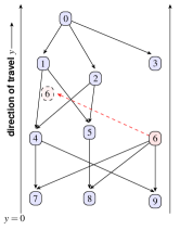
Figure 5: Information flow in $Y$ axis with car $6$ changing
lanes with trajectory shown
by the red dashed line

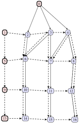
Figure 6: Influence graphs based on initial conditions in simulations Dashed lines indicate $X$ graph. Solid lines represent $Y$ graph

VII Simulations

In this section we present some numerical simulations. In our numerical simulations we use the scenarios of changing formations, obstacle avoidance, and lane change. We use the initial conditions depicted by graphs in Figure 6 for $Y$ and $X$ axis motion respectively. Unidirectional communication for $X$ and $Y$ axis is assumed with an influence level of one. Cars $1,5,9,13$ indicate the boundary of the road in Figure 6. The maximum number of cars in each level is $4$. The angle of view for $Y$ axis is a $120$°cone and for $X$ axis it is a $180$°angle. The system parameters in (2) and (4) are set as follows: $b=0.4$ and $k=0.001$. The vertical spacing constant between consecutive levels is $g_{y}=50$ and horizontal spacing for cars in the same level is $g_{x}=30$.

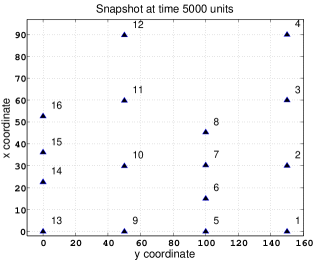
Figure 7: The $X$ vs $Y$ coordinates of cars are indicated at a time instant just before changing formations. The system is at equilibrium at this time

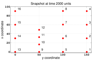
Figure 8: The $X$ vs $Y$ coordinates of cars are indicated at a time instant after formation has changed and the system has settled at equilibrium

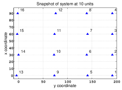
Figure 9: Figure shows the formation at the instant before car $6$ changes lanes

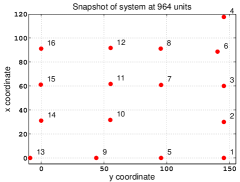
Figure 10: Figure shows the formation at the instant after car $6$ has changed lanes

VII-A Changing formations

When the equilibrium point of $X$ or $Y$ dynamics is changed we observe a change in the formation. We change vector $x_{f}$ in Remark IV.2 at different time instants to attain differing spacing between cars in the same level. Changing $x_{f}$ introduces impulse effects in the system in (2). Figures 7 and 8 demonstrates this effect. Cars $1$ to $4$ act as references and are spaced $30$ units from each other. Nodes $1,5,9,13$ represent the boundary. The ‘$\bullet$’ and ‘$\blacktriangle$’ represents the system a snapshot of the system at time $2000$ and $5000$ units respectively. The corresponding values of $x_{f}$ for which the figures are obtained is as follows. For time units of $5000$ units, $x_{f}^{T}=[\ 0\ 1\ 2\ 3\ 0\ 0.5\ 1\ 1.5\ 0\ 1\ 2\ 3\ 0\ 0.5\ 1\ 1.5]$. For time units of $2000$ units, $x_{f}^{T}=[\ 0\ 1\ 2\ 3\ 0\ 1\ 2\ 3\ 0\ 0.5\ 1\ 1.5\ 0\ 1\ 2\ 3\ ]$.

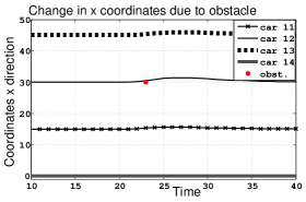
Figure 11: Trajectories of cars in $X$ direction changing due to the obstacle

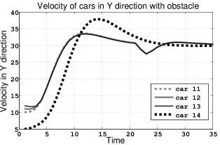
Figure 12: Velocities in $Y$ direction are plotted as function of time. The deviation is due to the obstacle

VII-B Obstacle avoidance

Here we show the impact of a stationary obstacle on the convoy. In our simulation the obstacle affects all cars below cars in level $2$, i.e. cars $10$ onwards. Figure 11 plots deviation of $x$ coordinates with respect to time. In Figure 11 the red star denotes the stationary obstacle. Car $12$ goes around the obstacle. This causes a change in position and velocity of cars $11$ and $13$ in the same level. Note that car $11$ has moved towards the obstacle, this is caused due to the control law forcing car $11$ to maintain a fixed distance with respect car $12$ and the obstacle.

Figure 12 shows the change in $Y$ velocities due to the obstacle.The black dotted trajectory is the reference trajectory in the absence of an obstacle. As cars $11$ to $13$ sense the obstacle their velocities drop as shown in the Figure. This drop causes a deviation in the $y$ coordinates of the cars. We now present the case for a particular car arbitrarily changing $x$ coordinates within the formation.

VII-C Lane change

For this example, car $6$ changes lanes from the left to the right in the formation. In doing so car $6$ has moved from one level below to one level above in the formation. Figure 9 shows the formation before lane change. As car $6$ changes lane other cars are also affected. This can be seen in Figure 10 in which cars $7,8$ are moving closer to car $5$. Cars $10,11$ are moving closer to cars $5,7,8$ in $Y$ direction. Note that $x_{f}$ has not been changed for level $2$ even after car $6$ has moved out hence the spacing is remaining same as before.

References

- [1] R. B. Bapat, Graph and Matrices, New Delhi:Hindustan Book Agency and Springer-Verlag,2010.
- [2] S. Boyd, L. E. Ghaoui, E. Feron, and V. Balakrishnan, Linear Matrix Inequalities in System and Contol Theory, Philadelphia:SIAM, 1994.
- [3] K. Chu, Decentralized Control of High-Speed Vehicular Strings, Transportation Science, Vol. 8, no. 4, pages 361-384, 1974.
- [4] J. A. Fax and R. M. Murray, Information Flow and Cooperative Control of Vehicle Formations, IEEE Transactions on Automatic Control, Vol. 49, no. 9, pages 1465-1476, 2004.
- [5] D. C. Gazis, R. Herman, and R. Rothery, Nonlinear Follow-the-leader Models of Traffic Flow, Operations Research, Vol. 9, no. 4, pages 545-567, 1961.
- [6] D. Gerlough and M. Huber, Traffic Flow Theory: A Monograph, 1975.
- [7] D. L. Gerlough and M. J. Huber, Traffic Flow Theory, Transportation Research Board Special Report, Washington D.C., 1975.
- [8] C. Hatipoglu, U. Azganer, and K. A. Redmill, Automated Lane Change Controller Design, IEEE Transactions on Intelligent Transportation Systems, Vol. 4, no. 1, pages 13-22, 2003.
- [9] D. Helbing, Improved Fluid Dynamic Model for Vehicular Traffic, Physical Review E, Vol. 51, no. 4, pages 3164-3169, 1995.
- [10] A. Jadbabaie, J. Lin, and A. S. Morse, Coordination of Groups of Mobile Autonomous Agents Using Nearest Neighbor Rules, IEEE Transactions on Automatic Control, Vol. 48, no. 6, pages 988-1001, 2003.
- [11] A. Klar and R. Wegener, A Heirarchy of Models for Multilane Vehicular Traffic I: Modeling, SIAM Journal of Applied Mathematics, Vol. 59, no. 3, pages 983-1001, 1999.
- [12] V. Lakshmikantham, D. D. Bainov, and P. S. Simeonov, Theory of Impulsive Differential Equations, Series in Modern Applied Mathematics, Vol. 6, World Scientific Publishing Co. Pte. Ltd, 1989.
- [13] F. Laquai, C. Gusmini, M. Tonnis, G. Rigoll and G. Klinker, A Multi Lane Car Following Model for Cooperative ADAS IEEE Annual Conference on Intelligent Transportation Systems, The Hague, The Netherlands, 2013.
- [14] J. A. Laval and C. F. Daganzo, Lane-changing in Traffic Streams, Transportation Research Part B: Methodological, Vol.40, no. 3, pages 251-264, 2006.
- [15] D. Liberzon, Switching in Systems and Control, Boston:Brikhuaser, 2003.
- [16] G. Michaletzky and L. Gerencser, BIBO Stability of Linear Switching Systems, IEEE Transactions on Automatic Control, Vol. 47, no. 11, 2002.
- [17] L. Moreau, Stability of Multi-agent Systems with Time-dependent Communication Links, IEEE Transactions on Automatic Control, Vol. 50, no. 2, pages 169-182, 2005.
- [18] R. Olfati-Saber and R.M. Murray, Distributed Structural Stabilization and Tracking for Formations of Dynamic Multi-agents Proceedings of the 41st IEEE Conference on Decision and Control, Las Vegas, NV, 2002.
- [19] R. Olfati-Saber and R. M. Murray, Consensus Problems in Networks of Agents with Switching Topology and Time-delays, IEEE Transactions on Automatic Control, Vol. 49, no. 9, pages 1520-1533, 2004.
- [20] R. Olfati-Saber and R. M. Murray, Flocking with Obstacle Avoidance: Cooperation with Limited Communication in Mobile Networks, Proceedings of the IEEE Conference on Decision and Control, Maui, HI, pages 2022-2028, 2003.
- [21] A. Pant, P. Seiler, and K. Hedrick, Mesh Stability of Look-Ahead Interconnected Systems, IEEE Transactions on Automatic Control, Vol. 47, no. 2, pages 403-407, 2002.
- [22] H. J. Payne, FREFLO: A Macroscopic Simulation Model of Freeway Traffic, Transportation Research Record 722, pages 68-77, 1979.
- [23] W. Ren and R. W. Beard, Consensus Seeking in Multiagent Systems Under Dynamically Changing Interaction Topologies, IEEE Transactions on Automatic Control, Vol. 50, no. 5,pages 655-661, 2005.
- [24] W. Ren and R. W. Beard, Distributed Consensus in Multi-vehicle Cooperative Control, London:Springer-Verlag, 2008.
- [25] W. Ren and E. Atkins, Distributed Multi-vehicle Coordinated Control via Local Information Exchange, International Journal of Robust and Nonlinear Control, Vol. 17, no. 10-11, pages 1002-1033, 2007.
- [26] S. Roy, A. Saberi, and K. Herlugson, Formation and Alignment of Distributed Sensing Agents with Double-Integrator Dynamics and Actuator Saturation, Sensor Network Applications, IEEE Press, New York, 2004.
- [27] P. Seiler, A. Pant, and J.K. Hedrick, Preliminary Investigation of Mesh Stability for Linear Systems, Proceedings of the ASME: DSC Division 67, pages 359-364, 1999.
- [28] Q. Song and J. Zhang, Novel Results on Mesh Stability for a Class of Vehicle Following System with Time Delays Advances in Neural Networks - ISNN, Shenyang, China, 2012.
- [29] D. Swaroop and J. K. Hedrick, String Stability of Interconnected Systems, IEEE Transactions on Automatic Control, Vol. 41, no. 3, pages 349-357, 1996.
- [30] H. Tanner, V. Kumar and G. Pappas, Stability Properties of Interconnected Vehicles, Proceedings of the 15th International Symposium on Mathematical Theory of Networks and Systems, South Bend IN, 2002.
- [31] Z. Wen-xing and J. Lei, Analysis of a New Car-following Model with a Consideration of Multi-interaction of Preceding vehicles, IEEE Intelligent Transportation Systems Conference, Seattle, WA, USA, 2007.
- [32] T. Yang, Impulsive Control Theory, Lecture notes in Control and Information Sciences, Vol. 272, Heidelberg:Springer, 2001.
- [33] H. Ye, A. N. Michel, and L. Hou, Stability Theory for Hybrid Dynamical Systems IEEE Transactions on Automatic Control, Vol. 43, no. 4, pages 461-475, 1998.