Numerical solution for a general class of nonlocal nonlinear wave equations

Abstract

A class of nonlocal nonlinear wave equation arises from the modeling of a one dimensional motion in a nonlinearly, nonlocally elastic medium. The equation involves a kernel function with nonnegative Fourier transform. We discretize the equation by using Fourier spectral method in space and we prove the convergence of the semidiscrete scheme. We then use a fully-discrete scheme, that couples Fourier pseudo-spectral method in space and 4th order Runge-Kutta in time, to observe the effect of the kernel function on solutions. To generate solitary wave solutions numerically, we use the Petviashvili’s iteration method.

1 Introduction

In this article, we study the nonlocal nonlinear wave equation

$$u_{tt}=\beta\ast(u+g(u))_{xx},$$ (1.1)

where $g$ is a nonlinear function of $u$. Here $\ast$ denotes the convolution in spatial domain and the kernel function $\beta(x)$ is an integrable function. Equation (1.1) has been derived to model one-dimensional motion in an infinite medium with nonlinear and nonlocal elastic properties from nonlocal elasticity theory [3, 4]. Duruk et. al. have proved the global existence of the Cauchy problem corresponding to (1.1) together with initial conditions

$$u(x,0)=\phi(x),~{}~{}~{}~{}u_{t}(x,0)=\psi(x)$$ (1.2)

with enough smoothness on the initial data, and continuity condition on the nonlinear function $g$ in [3]. They assume that the Fourier transform of the kernel function $\beta(x)$ satisfies

$$0\leq\widehat{\beta}(k)\leq C(1+k^{2})^{-r/2},~{}~{}\mbox{for~{}all~{}}k\in\mathbb{R}$$ (1.3)

for some constant $C>0$, $r\in\mathbb{R}$ and $r\geq 2$. Suppose that $u$ and all its derivatives converge to zero sufficiently and rapidly as $x\rightarrow\pm\infty$. For the solutions of the eq. (1.1) subjected to these boundary conditions the conserved quantity (energy) [3] is given by

$$E\left(t\right)=\left\|Pu_{t}\right\|^{2}+\left\|u\right\|^{2}+2\int_{\mathbb{R}}G\left(u\right)dx.$$

Here the operator $P$ is defined as

$$Pv=\mathcal{F}^{-1}\left(\frac{\hat{v}\left(k\right)}{\left|k\right|\sqrt{\widehat{\beta}(k)}}\right)$$

where $\mathcal{F}^{-1}$ is the inverse Fourier transform and $\displaystyle G(u)=\int_{0}^{u}g(s)ds$.

For some suitable choice of the kernel function $\beta(x)$ the equation (1.1) becomes well-known nonlinear wave equations. In the case of the Dirac delta function, $\beta=\delta$, the condition (1.3) is satisfied by $r=0$ and the equation (1.1) is the well-known nonlinear wave equation

$$u_{tt}-u_{xx}=g\left(u\right)_{xx}.$$

Choosing the exponential kernel [6], $\beta(x)={\frac{1}{2}}e^{-|x|}$, the equation (1.1) becomes the improved Boussinesq equation (IBq),

$$u_{tt}-u_{xx}-u_{xxtt}=(g(u))_{xx}~{}.$$

Since $\widehat{\beta}(k)=(1+k^{2})^{-1}$, we have $r=2$. A final example is the double-exponential kernel [9]

$$\beta(x)={\frac{1}{{2(c_{1}^{2}-c_{2}^{2})}}}(c_{1}e^{-|x|/c_{1}}-c_{2}e^{-|x|/c_{2}})$$

where $c_{1}$ and $c_{2}$ are real and positive constants. As $\widehat{\beta}(k)=(1+\eta_{1}k^{2}+\eta_{2}k^{4})^{-1}$ where $\eta_{1}=c_{1}^{2}+c_{2}^{2}$ and $\eta_{2}=c_{1}^{2}c_{2}^{2}$, we have $r=4$. In this case the equation (1.1) becomes the higher-order Boussinesq equation (HBq),

$$u_{tt}-u_{xx}-\eta_{1}u_{xxtt}+\eta_{2}u_{xxxxtt}=(g(u))_{xx}~{}.$$

For these special cases there are numerous studies in the literature both numerical and analytical (see [1] and [16] and the references there in). The existence and stability of solitary wave solutions of the nonlocal nonlinear wave equation (1.1) has been shown in a recent study [5]. The nonlocal term makes it harder to investigate the equation analytically. Therefore the numerical solution is important to understand the evolution of solutions in time and the effect of the kernel on the solutions.

The existence of the convolution integral and the condition (1.3) on the Fourier coefficients of the kernel function $\beta(x)$ make the spectral methods a natural choice for the numerical solution. Spectral methods are widely used for local equations. Some of the numerical studies using spectral methods for the nonlocal equations are as follows: In [11, 12], the authors have studied a class of nonlinear nonlocal dispersive wave equation by using the combination of Fourier Galerkin spectral method and explicit leap-frog scheme. In [8], the author has studied regularized Benjamin-Ono equation by using both Fourier Galerkin and Fourier collocation methods.

In the recent studies [1, 16] a Fourier pseudo-spectral method has been used for the numerical solutions of the IBq and HBq equations. Thus the efficiency of the method has been tested for the special cases of this class of nonlocal equations. Therefore in this study we use Fourier pseudo-spectral method, together with a fourth order Runge-Kutta method, to solve (1.1) numerically. In Section 2, we give notations and preliminaries. In Section 3, we prove the convergence of the semi-discrete scheme. In Section 4, we introduce a fully discrete scheme combining the Fourier pseudo-spectral method and fourth order Runge-Kutta method for space and time discretization, respectively. Although the exact forms of solitary wave solutions are known for the IBq and HBq equations, we do not have the exact form of the solitary wave solutions for the general nonlocal nonlinear wave equation. Therefore, we use the Petviashvili’s iteration method to construct the solitary wave profile numerically in Section 5. Finally, we present some numerical implementation of the method in Section 6.

2 Notations and preliminaries

We use the function space $L^{2}(\Omega)$ and the Sobolev space $H^{s}$. $(\cdot,\cdot)$ denotes the $L^{2}$ inner product and $\|\cdot\|$ is the corresponding norm defined, respectively as

$$(u,v)=\int_{\Omega}u(x)\overline{v(x)}dx,\hskip 10.0pt\mbox{and}\hskip 10.0pt\|u\|^{2}=(u,u)$$ (2.4)

where $\Omega=(-L,L)$. The periodic Sobolev space $H^{s}_{p}(\Omega)$ is equipped with the norm

$$\|u\|_{s}^{2}=\sum_{k=-\infty}^{\infty}(1+k^{2})^{s}|\hat{u}_{k}|^{2}.$$ (2.5)

The Banach space $X_{s}=C^{1}([0,T];H^{s}_{p}(\Omega))$ is the space of all continuous functions in $H^{s}_{p}(\Omega)$ whose distributional derivative is also in $H^{s}_{p}(\Omega)$, with norm $~{}\left\|u\right\|_{X_{s}}^{2}=\displaystyle\max_{t\in[0,T]}(\left\|u(t)\right\|_{s}^{2}+\left\|u_{t}(t)\right\|_{s}^{2})$. Here the Fourier coefficients of a function is given as

$$\hat{u}_{k}=\displaystyle\frac{1}{2L}\int_{\Omega}u(x)e^{{ik\pi x}/{L}}dx.$$

For a positive integer $N$ the space of trigonometric polynomials of degree $N/2$ is

$$S_{N}=\mbox{span}\{e^{{ik\pi x}/{L}}|-N/2\leq k\leq N/2-1\}$$ (2.6)

The operator $P_{N}:L^{2}(\Omega)\rightarrow S_{N}$ denotes the orthogonal projection defined as

$$P_{N}u(x)=\sum_{k=-N/2}^{N/2-1}\hat{u}_{k}~{}e^{{ik\pi x}/{L}}.$$ (2.7)

So that the projection operator $P_{N}$ has the property

$$(u-P_{N}u,\varphi)=0,\hskip 20.0pt\forall\varphi\in S_{N}.$$ (2.8)

$P_{N}$ commutes with derivative in the distributional sense:

$$D_{x}^{n}P_{N}u=P_{N}D_{x}^{n}u\hskip 20.0pt\mbox{and}\hskip 20.0ptD_{t}^{n}P_{N}u=P_{N}D_{t}^{n}u.$$ (2.9)

Here $D_{x}^{n}$ and $D_{t}^{n}$ stand for the $n$th-order classical partial derivative with respect to $x$ and $t$, respectively. In the rest of study, $C$ denotes a generic constant.

3 The semi-discrete scheme

In this section we present a Fourier pseudo-spectral method for the spatial discretization and then we prove the convergence of the semi-discrete scheme. The equation (1.1) equivalently can be written as

$$u_{tt}={\cal H}[u+g(u)]_{xx},$$ (3.1)

where ${\cal H}$ is the convolution operator given by

$${\cal H}v(x)=\int_{\Omega}\beta(x-y)v(y)dy.$$

Then, the equation (3.1) becomes

$${\cal H}^{-1}u_{tt}=[u+g(u)]_{xx}.$$ (3.2)

We define the operator ${\cal H}^{-1}$ as ${\cal H}^{-1}v={\cal F}^{-1}({\hat{v}(k)}/{\hat{\beta}(k)})$ where ${\cal F}^{-1}$ is the inverse Fourier transform. The semi-discrete Fourier pseudo-spectral scheme for (3.2) with the initial conditions (1.2) are given as

$${\cal H}^{-1}u^{N}_{tt}=u^{N}_{xx}+P_{N}(g(u^{N}))_{xx},$$ (3.3)

$$u^{N}(x,0)=P_{N}\phi(x),\hskip 20.0ptu^{N}_{t}(x,0)=P_{N}\psi(x)$$ (3.4)

where $u^{N}(x,t)$ is a function from $[0,T]$ to $S_{N}$. We use the following lemmas for the convergence proof of the semi-discrete scheme:

Lemma 3.1.

[2, 14] For any real $0\leq\mu\leq s$, there exists a constant $C$ such that

$$\|u-P_{N}u\|_{\mu}\leq CN^{\mu-s}\|u\|_{s},\hskip 20.0pt\forall u\in H^{s}_{p}(\Omega).$$ (3.5)

Lemma 3.2.

[15] Assume that $f\in C^{k}(\mathbb{R})$, $u,v\in H^{s}(\Omega)\cap L^{\infty}(\Omega)$ and $k=[s]+1$, where $s\geq 0$. Then we have

$$\|f(u)-f(v)\|_{s}\leq C(M)\|u-v\|_{s}$$ (3.6)

if $\|u\|_{\infty}\leq M,\|v\|_{\infty}\leq M,\|u\|_{s}\leq M$ and $\|v\|_{s}\leq M$, where $C(M)$ is a constant dependent on $M$ and $s$.

Lemma 3.3.

Let $r\geq 2$ and $v\in H^{r/2}(\Omega)$. If the kernel function $\beta(x)$ satisfies the condition (1.3), then there exists a constant $C$ such that

$$\|v\|_{r/2}\leq C\|{\cal H}^{-1/2}v\|.$$ (3.7)

Proof.

The proof directly follows from the definition of the operator ${\cal H}^{-1/2}$ and the condition (1.3). ∎

The following theorem states our main result.

Theorem 3.4.

Let $s\geq r/2$, $g\in C^{2}(\mathbb{R})$ and $u(x,t)$ be the solution of the periodic initial value problem (1.1)-(1.2) satisfying $u(x,t)\in C^{1}([0,T];H^{s}_{p}(\Omega))$ for any $T>0$ and $u^{N}(x,t)$ be the solution of the semi-discrete scheme (3.3)-(3.4). There exists a constant $C$, independent of $N$, such that

$$\|u-u^{N}\|_{X_{r/2}}\leq C(T)N^{r/2-s}\|u\|_{X_{s}}$$ (3.8)

for the initial data $\phi,\psi\in H^{s}_{p}(\Omega)$.

Proof.

To estimate the term $\displaystyle\|u-u^{N}\|_{X_{r/2}}$ we first use the triangle inequality to write

$$\|u-u^{N}\|_{X_{r/2}}\leq\|u-P_{N}u\|_{X_{r/2}}+\|P_{N}u-u^{N}\|_{X_{r/2}}.$$ (3.9)

For the first term on the right-hand side, we use Lemma 3.1 and the fact that the projection operator $P_{N}$ commutes with the differentiation, to obtain the following estimate

$$\|(u-P_{N}u)_{t}(t)\|_{r/2}\leq CN^{r/2-s}\|u_{t}(t)\|_{s},$$ (3.10)

for $s\geq r/2$. Thus, we bound the first term in (3.9) as

$$\|u-P_{N}u\|_{X_{r/2}}\leq CN^{r/2-s}\|u\|_{X_{s}}.$$ (3.11)

To estimate the second term $\|P_{N}u-u^{N}\|_{X_{r/2}}$ at the right-hand side of the inequality (3.9), we subtract the equation (3.3) from (3.1) and take the inner product with $\varphi\in S_{N}$;

$$\left({\cal H}^{-1}(u-u^{N})_{tt}-(u-u^{N})_{xx}-(g(u)-P_{N}g(u^{N}))_{xx},~{}\varphi\right)=0.$$ (3.12)

Orthogonality of the projection operator $P_{N}$ gives

$$\left({\cal H}^{-1}(u-P_{N}u)_{tt},~{}\varphi\right)=0$$ (3.13)

for all $\varphi\in S_{N}$, using this result together with (2.8) the equation (3.12) turns to

$$\left({\cal H}^{-1}(P_{N}u-u^{N})_{tt}-(P_{N}u-u^{N})_{xx}-(g(u)-P_{N}g(u^{N}))_{xx},~{}\varphi\right)=0.$$ (3.14)

We now set $\varphi=(P_{N}u-u^{N})_{t}$ in (3.14). Since ${\cal H}^{-1/2}$ is a self-adjoint operator, we have

$$\left({\cal H}^{-1}(P_{N}u-u^{N})_{tt},~{}(P_{N}u-u^{N})_{t}\right)=\frac{1}{2}\frac{d}{dt}\|{\cal H}^{-1/2}(P_{N}u-u^{N})_{t}(t)\|^{2}.$$ (3.15)

Spatial periodicity and the integration by parts yield

$$\left((P_{N}u-u^{N})_{xx},~{}(P_{N}u-u^{N})_{t}\right)=-\frac{1}{2}\frac{d}{dt}\|(P_{N}u-u^{N})_{x}(t)\|^{2}.$$ (3.16)

For the nonhomogeneous term in (3.14) we use the Cauchy-Schwarz inequality, triangle inequality and Lemma 3.2. Therefore we have

$$\left((g(u)-g(u^{N}))_{xx},(P_{N}u-u^{N})_{t}\right)$$

$$\leq\left|\left((g(u)-g(u^{N}))_{x},~{}(P_{N}u-u^{N})_{xt}\right)\right|$$

$$\leq\|(g(u)-g(u^{N}))_{x}\|~{}\|(P_{N}u-u^{N})_{xt}(t)\|$$

$$\leq\frac{1}{2}\left(\|g(u)-g(u^{N})\|_{1}^{2}+\|(P_{N}u-u^{N})_{t}(t)\|_{1}^{2}\right)$$

$$\leq C\left(\|(u-u^{N})(t)\|_{1}^{2}+\|(P_{N}u-u^{N})_{t}(t)\|_{1}^{2}\right)$$

$$\leq C\left(\|(u-P_{N}u)(t)\|_{r/2}^{2}+\|(P_{N}u-u^{N})(t)\|_{r/2}^{2}+\|(P_{N}u-u^{N})_{t}(t)\|_{1}^{2}\right)$$

for $r\geq 2$. Combining the results of (3.15)-(LABEL:nonhom) the equation (3.14) becomes

$$\frac{1}{2}\frac{d}{dt}\left(\|{\cal H}^{-1/2}(P_{N}u-u^{N})_{t}(t)\|^{2}+\|(P_{N}u-u^{N})_{x}(t)\|^{2}\right)$$

$$\hskip 15.0pt\leq C\left(\|(u-P^{N}u)(t)\|_{r/2}^{2}+\|(P^{N}u-u)(t)\|_{r/2}^{2}+\|(P_{N}u-u^{N})_{t}(t)\|_{1}^{2}\right).$$

We now add the terms

$$\left(P_{N}u-u^{N},(P_{N}u-u^{N})_{t}\right)+\sum_{i=2}^{r/2}\left(D^{i}_{x}(P_{N}u-u^{N}),D^{i}_{x}(P_{N}u-u^{N})_{t}\right)$$

to both sides of the inequality (3) and use that

$$\left(D^{i}_{x}(P_{N}u-u^{N}),D^{i}_{x}(P_{N}u-u^{N})_{t}\right)=\frac{1}{2}\frac{d}{dt}\|D^{i}_{x}(P_{N}u-u^{N})(t)\|^{2},$$

and

$$\left(D^{i}_{x}(P_{N}u-u^{N}),D^{i}_{x}(P_{N}u-u^{N})_{t}\right)\leq C\left(\|D^{i}_{x}(P_{N}u-u^{N})(t)\|^{2}+\|D^{i}_{x}(P_{N}u-u^{N})_{t}(t)\|^{2}\right).$$

Using all these results and Lemma 3.3, the inequality (3) becomes

$$\frac{1}{2}\frac{d}{dt}\left(\|{\cal H}^{-1/2}(P_{N}u-u^{N})_{t}(t)\|^{2}+\|(P_{N}u-u^{N})(t)\|_{r/2}^{2}\right)$$

$$\hskip 40.0pt\leq C\left(\|(u-P_{N}u)(t)\|_{r/2}^{2}+\|(P_{N}u-u^{N})(t)\|_{r/2}^{2}+\|(P_{N}u-u^{N})_{t}(t)\|_{r/2}^{2}\right)$$

$$\hskip 40.0pt\leq C\left(\|(u-P_{N}u)(t)\|_{r/2}^{2}+\|(P_{N}u-u^{N})(t)\|_{r/2}^{2}+\|{\cal H}^{-1/2}(P_{N}u-u^{N})_{t}(t)\|^{2}\right).$$

Note that $\|{\cal H}^{-1/2}(P_{N}u-u^{N})_{t}(0)\|^{2}=\|(P_{N}u-u^{N})(0)\|^{2}=0$. Using Gronwall Lemma followed by Lemma 3.1 we conclude that

$$\|{\cal H}^{-1/2}(P_{N}u-u^{N})_{t}(t)\|^{2}+\|(P_{N}u-u^{N})(t)\|_{r/2}^{2}$$

$$\hskip 20.0pt\leq\int_{0}^{t}\|u(\tau)-P_{N}u(\tau)\|_{r/2}^{2}~{}e^{C(t-\tau)}d\tau$$

$$\hskip 20.0pt\leq C(T)~{}N^{r-2s}\int_{0}^{t}\|u(\tau)\|_{s}^{2}~{}d\tau$$ (3.19)

for $s\geq r/2$. Thanks to Lemma 3.3, we know that

$$\|(P_{N}u-u^{N})_{t}(t)\|_{r/2}^{2}+\|(P_{N}u-u^{N})(t)\|_{r/2}^{2}$$

$$\hskip 30.0pt\leq\|{\cal H}^{-1/2}(P_{N}u-u^{N})_{t}(t)\|^{2}+\|(P_{N}u-u^{N})_{t}(t)\|_{r/2}^{2}.$$

Finally, we have the estimate

$$\|P_{N}u-u^{N}\|_{X_{r/2}}\leq C(T)N^{r/2-s}~{}\|u\|_{X_{s}}.$$ (3.20)

The inequalities (3.11) and (3.20) give the estimation for (3.9), which completes the proof of Theorem 3.4. ∎

Note that the result of the Theorem 3.4 coincides with the special cases of the equation (1.1), the IBq and HBq equations, for which $r=2$ and $r=4$, respectively [1, 16].

4 The fully-discrete scheme

We solve the equation (1.1) by combining a Fourier pseudo-spectral method for the space component and a fourth-order Runge Kutta scheme (RK4) for time. If the spatial period $[-L,\,L]$ is normalized to $[0,2\pi]$ using the transformation $X=\pi(x+L)/L$, the equation (1.1) with $g(u)=u^{p}$ becomes

$$u^{N}_{tt}=\left(\frac{\pi}{L}\right)^{2}(\beta\ast(u^{N}+(u^{N})^{p}))_{XX}.$$ (4.1)

The space interval $[0,2\pi]$ is divided into $N$ equal subintervals with grid spacing $\Delta X=2\pi/N$, where the integer $N$ is even. The spatial grid points are then given by $X_{j}=2\pi j/N$, $j=0,1,2,...,N$. The time interval $[0,T]$ is divided into $M$ equal subintervals with grid spacing $\Delta t=T/M$. The approximate solution to $u^{N}(X_{j},t)$ is denoted by $U_{j}(t)$. Applying the discrete Fourier transform to the equation (4.1) we have

$$(\tilde{U}_{k})_{tt}=-\left(\frac{\pi k}{L}\right)^{2}\,\tilde{\beta}_{k}\,[\,\tilde{U}_{k}+(\tilde{U}^{p})_{k}\,].$$ (4.2)

The above equation can be written as an ordinary differential equation system

$$(\tilde{U}_{k})_{t}=\tilde{V}_{k}$$ (4.3)

$$(\tilde{V}_{k})_{t}=-(\pi k/L)^{2}\,\tilde{\beta}_{k}\,[\,\tilde{U}_{k}+(\tilde{U}^{p})_{k}\,].$$ (4.4)

In order to handle the nonlinear term we use a pseudo-spectral approximation. We use the fourth order Runge-Kutta method to solve the resulting ODE system (4.3)-(4.4) in time. Finally, we find the approximate solution by using the inverse discrete Fourier transform.

5 The Petviashvili’s iteration method

One of the most effective numerical methods to generate solitary wave solution was first proposed by V. I. Petviashvili for the Kadomtsev-Petviashvili equation in [13]. Since we do not have the exact form of the solitary wave solutions for the general nonlocal nonlinear wave equation, we use the Petviashvili’s iteration method [10, 13, 17] to construct the solitary wave solution numerically.

The solitary wave solutions of (1.1) are of the form $u(x,t)=\phi(x-ct)$, where $c$ is the propagation speed of a solitary wave. Substituting this solution into (1.1) and then integrating twice and using the asymptotic boundary conditions, we have

$$c^{2}\phi=[\beta*(\phi+\phi^{p})].$$ (5.1)

If we use the Fourier transform,

$$u(x)=\frac{1}{2\pi}\int_{-\infty}^{\infty}\hat{u}(k)e^{ikx}dk,\hskip 30.0pt\hat{u}(k)=\int_{-\infty}^{\infty}u(x)e^{-ikx}dx,$$ (5.2)

the eq. (5.1) can be written as

$$[c^{2}-\hat{\beta}(k)]\hat{\phi}(k)=\hat{\beta}(k)\widehat{\phi^{p}}(k).$$ (5.3)

A simple iterative algorithm for numerical calculation of $\hat{\phi}(k)$ for the above eq. can be proposed in the form

$$\hat{\phi}_{n+1}(k)=\frac{\hat{\beta}(k)}{c^{2}-\hat{\beta}(k)}\widehat{\phi_{n}^{p}}(k).$$ (5.4)

where $\hat{\phi}_{n}(k)$ is the Fourier transform of $\phi_{n}(x)$ which is the $n^{th}$ iteration of the numerical solution. Although there exists a fixed point $\hat{\phi}_{n}(k)$ of the eq. (5.1), the algorithm (5.4) diverges. To ensure the convergence, we add a stabilizing factor $M_{n}$ as in [13]. The new algorithm for the nonlocal nonlinear wave eq. can be proposed in the form

$$\hat{\phi}_{n+1}(k)=M_{n}^{\gamma}\frac{\hat{\beta}(k)}{c^{2}-\hat{\beta}(k)}\widehat{\phi^{p}_{n}}(k).$$ (5.5)

where the stabilizing factor is

$$M_{n}=\frac{\int_{-\infty}^{\infty}(c^{2}-\hat{\beta}(k))~{}[\hat{\phi}_{n}(k)]^{2}dk}{\int_{-\infty}^{\infty}\hat{\beta}(k)\widehat{\phi^{p}_{n}}(k)\hat{\phi}_{n}(k)dk}$$ (5.6)

and $\gamma$ is a free parameter. Note that we can only construct the solitary wave solutions for the nonlocal nonlinear wave eq. under the assumption

$$c^{2}-\hat{\beta}(k)\neq 0.$$ (5.7)

for all $k\in\mathbb{R}$.

6 Numerical implementation

In this section we present some numerical results to understand the effect of the kernel function $\beta(x)$ on the solution. Throughout the section we consider the quadratic nonlinearity, i.e. $g(u)=u^{2}$. In the first numerical experiment, we consider the general kernel function satisfying (1.3) whose Fourier transform is

$$\hat{\beta}(k)=\frac{1}{1+k^{2}+\eta k^{2}\sin(k^{2})}.$$ (6.1)

Here $\eta$ is a positive parameter. Note that $\hat{\beta}(k)$ is a decreasing function of $k$. Therefore, the speed must be chosen as $c^{2}>1$ to satisfy the condition (5.7). First, we construct a solitary wave solution corresponding to the above kernel for $\eta=1$ by using the Petviashvili’s iteration method. For this aim, we use the pseudo-spectral approximation for the eq. (5.5). The initial guess is

$$\phi_{0}(x)=e^{-x^{2}}$$ (6.2)

and we take the the speed as $c=1.08$. In the left panel of Figure 1, we show the solitary wave profile of the eq. (1.1) on the interval $[-100,100]$ with $N=1024$. In the right panel of Figure 1, we show the variation of the logarithm of the residual error with the number of iterations. Here the residual error is defined as

$$\mbox{Residual error}=\|M\phi_{n}\|_{\infty}$$ (6.3)

where

$$M\phi=c^{2}\phi-[\beta*(\phi+\phi^{p})].$$ (6.4)

We observe that the fastest convergence occurs when $\gamma=2$.

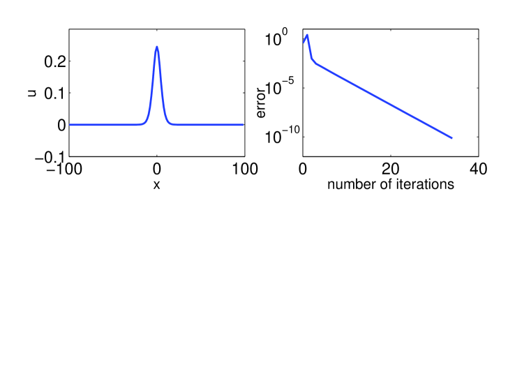
Figure 1: The numerical solitary wave profile for the speed $c=1.08$ and the variation of the logarithm of the residual error with the number of iterations.

To investigate the time evolution of the wave, the initial condition $u(x,0)$ is chosen as the profile constructed by the Petviashvili’s iteration method (left panel of Figure 1). On the other hand, we also need the initial condition $u_{t}(x,0)$. The traveling wave solutions of the eq. (1.1) are given in the form $u(x,t)=\phi(x-ct)$. Therefore, the initial condition $u_{t}(x,0)$ is chosen as $u_{t}(x,0)=-cu_{x}(x,0)$ and the $x$-derivative is evaluated by using discrete Fourier transform. In the left panel of Figure 2, we illustrate the time evolution of the wave corresponding to these initial conditions. In the right panel of Figure 2, the variation of the change in the conserved quantity $E$ (energy) with time is presented.

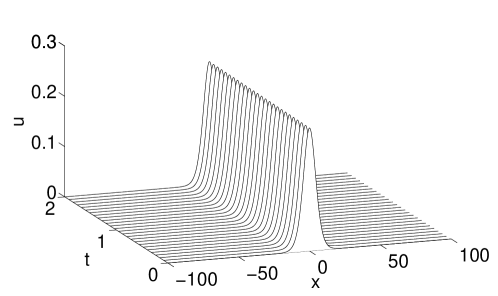
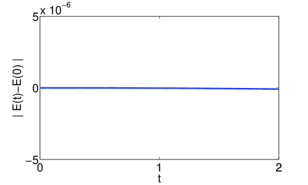
Figure 2: The time evolution of the wave generated by Petviashvili’s iteration method (left panel) and the variation of the change in the conserved quantity $E$ (energy) with time (right panel).

We point out that the kernel (6.1) corresponds to the kernel giving rise to the IBq equation when $\eta=0$. In this case, if the nonlinearity is quadratic, the relation between the amplitude $A$ and the speed parameter $c$ is given by $A=1.5(c^{2}-1)$. In Figure 3, the dashed line shows the variation of the amplitude with the speed parameter for the IBq equation. The solid lines show the variation of the amplitude with the speed parameter corresponding to kernel (6.1) for $\eta=10$, $\eta=5$, $\eta=1$ and $\eta=0.1$.

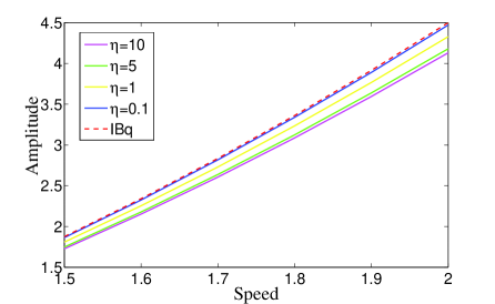
Figure 3: Variation of the amplitude with the speed parameter for the IBq eq. and for the nonlocal nonlinear wave eq. with the kernel (6.1) for various values of $\eta$.

The question arises naturally how the solitary wave solutions of the nonlocal nonlinear wave equation behaves when $\eta\rightarrow 0^{+}$. For this aim, we perform some numerical tests for various values of $\eta$ by using the initial condition

$$u(x,0)=\frac{1}{4}{\mbox{sech}}^{2}(\frac{x}{\sqrt{28}}),$$ (6.5)

$$v(x,0)=\frac{1}{2}\,{\mbox{sech}}^{2}\left(\frac{x}{\sqrt{28}}\right)\,\tanh\left(\frac{x}{\sqrt{28}}\right).$$ (6.6)

The given initial condition corresponds to the exact solitary wave solution of the IBq equation. The problem is solved on the interval $-100\leq x\leq 100$ for times up to $T=10$. In Figure $4$, the solid line shows the exact solution of the IBq equation given in [1] which corresponds to the initial conditions (6.5)-(6.6). The dashed lines show the numerical solution of the nonlocal nonlinear wave equation obtained by the kernel function whose Fourier transform is given by (6.1) for $\eta=10$, $\eta=5$, $\eta=1$ and $\eta=0.1$ at the final time $T=10$. The numerical tests show that the solutions of the nonlocal nonlinear wave equation converge to the solitary wave solution of the IBq equation as $\eta\rightarrow 0^{+}$.

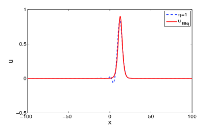
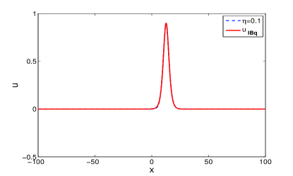
Figure 4: The exact solution of the IBq equation and the numerical solution of the nonlocal nonlinear wave equation with (6.1).

Next, we consider the kernel function whose Fourier transform is

$$\hat{\beta}(k)=\frac{1}{1+k^{2}+k^{4}}+\frac{\mu}{1+k^{4}}.$$ (6.7)

Here $\mu$ is a positive parameter. As $\hat{\beta}(k)$ is a decreasing function of $k$, the speed must be chosen as $c^{2}>1+\mu$ to satisfy the condition (5.7). This kernel corresponds to the kernel giving rise to the HBq equation with $\eta_{1}=\eta_{2}=1$ when $\mu=0$. To observe the behavior of the solutions as $\mu\rightarrow 0^{+}$, we perform some numerical tests for various values of $\mu$ by using the initial condition

$$u(x,0)=\frac{105}{266}\,{\mbox{sech}}^{4}(\frac{x}{2\sqrt{13}}),$$ (6.8)

$$v(x,0)=\frac{105}{133^{3/2}}\,{\mbox{sech}}^{4}\left(\frac{x}{2\sqrt{13}}~{}\right)\,\tanh\left(\frac{x}{2\sqrt{13}}~{}\right).$$ (6.9)

The given initial condition gives rise to the exact solitary wave solution of the HBq equation. In Figure 5, the solid line shows the exact solution of the HBq equation given in [16] which corresponds to the initial conditions (6.8)-(6.9). The dashed lines show the numerical solution of the nonlocal nonlinear wave equation obtained by the kernel function whose Fourier transform is given in (6.7) for $\mu=10$, $\mu=5$, $\mu=1$ and $\mu=0.1$ at the final time $T=10$. The numerical tests show that the solutions of the nonlocal nonlinear wave equation converge to the the solution of the HBq equation as $\mu\rightarrow 0^{+}$.

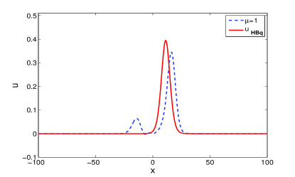
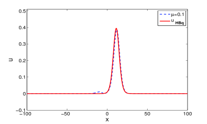
Figure 5: The exact solution of the HBq equation and the numerical solution of the nonlocal nonlinear wave equation with (6.7).

For the last experiment, our aim is to investigate whether the above convergence property is also valid for the blow-up solutions or not. The blow-up theorem for the nonlocal nonlinear wave equation given in [3] has been restated as follows:

Theorem 6.1.

(Theorems $3.4$ and $5.2$ of [3]) Let $s>1/2$ and $r\geq 2$. Then, there is some $T>0$ such that the Cauchy problem (1.1)-(1.2) is well-posed with solution in $C^{2}([0,T],H^{s}(\Omega))$ for initial data $\phi,\psi\in H^{s}(\Omega)$. Furthermore, suppose that $P\phi,P\psi\in L^{2}(\Omega)$ and $~{}~{}G(\phi)\in L^{1}(\Omega)$. If there is some $\nu>0$ such that

$$p\,g\left(p\right)\leq 2\nu p^{2}+2\left(1+2\nu\right)G\left(p\right)\mbox{ for all }p\in\mathbb{R},$$

and the initial energy

$$E\left(0\right)=\left\|P\psi\right\|^{2}+\left\|\phi\right\|^{2}+2\int_{\mathbb{R}}G\left(\phi\right)dx<0~{},$$

then the solution $u$ of the Cauchy problem (1.1)-(1.2) blows up in finite time.

For the numerical tests, we use the kernel whose Fourier transform is given in (6.1) and we choose the initial conditions

$$\phi(x)=4\left(\frac{2x^{2}}{3}-1\right)e^{-\frac{~{}x^{2}}{3}},\hskip 30.0pt\psi(x)=\left(x^{2}-1\right)e^{-\frac{~{}x^{2}}{3}}$$ (6.10)

as in [7]. Thus, the conditions for the blow-up theorem are satisfied for $\nu=\frac{1}{4}$. The problem is solved on the interval $-10\leq x\leq 10$ for times up to $T=3$. In Figure 6, we present the variation of the $L_{\infty}$ norm of the numerical solution obtained by using the Fourier pseudo-spectral scheme. The numerical results strongly indicate that the blow-up time of the nonlocal nonlinear wave equation converges to $t^{*}\approx 1.8$, which is the blow-up time of the IBq equation, as $\eta\rightarrow 0^{+}$.

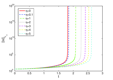
Figure 6: $L_{\infty}$ norm of the numerical solution for the increasing time.

Acknowledgement: This work has been supported by the Scientific and Technological Research Council of Turkey (TUBITAK) under the project MFAG-113F114. The authors gratefully acknowledge to the anonymous reviewers for the constructive comments and valuable suggestions which improved the original paper.

References

[1]
H. Borluk, G. M. Muslu, A Fourier pseudospectral method for a generalized
improved Boussinesq equation, Numer. Meth. Part. D. E. 31 (2015) 995–1008.
[2]
C. Canuto, A. Quarteroni, Approximation results for orthogonal polynomials in
Sobolev spaces, Math. Comp. 38 (1982) 67–86.
[3]
N. Duruk, H. A. Erbay, A. Erkip, Global existence and blow-up for a
class of nonlocal nonlinear Cauchy problems arising in elasticity,
Nonlinearity 23 (2010) 107–118.
[4]
N. Duruk, A. Erkip, H. A. Erbay, A higher-order Boussinesq equation in
locally non-linear theory of one-dimensional non-local
elasticity, IMA J. Appl. Math. 74 (2009) 97–106.
[5]
H. A. Erbay, S. Erbay, A. Erkip, Existence and stability of traveling waves for
a class of nonlocal nonlinear equations, J. Math. Anal. Appl. 425 (2015)
307–336.
[6]
A. C. Eringen, On differential equations of nonlocal elasticity and solutions
of screw dislocation and surface waves, J. Appl. Phys. 54 (1983) 4703–4710.
[7]
A. Godefroy, Blow-up solutions of a generalized Boussinesq equation, IMA
J. Numer. Anal. 60 (1998) 122–138.
[8]
H. Kalisch, Error analysis of a spectral projection of the regularized
Benjamin-Ono equation, BIT 45 (2005) 69–89.
[9]
M. Lazar, G. A. Maugin, E. C. Aifantis, On a theory of nonlocal elasticity of
bi-Helmholtz type and some applications, Int. J. Solids Struct. 43 (2006)
1404–1421.
[10]
D. E. Pelinovsky, Y. A. Stepanyants, Convergence of Petviashvili’s iteration
method for numerical approximation of stationary solutions of nonlinear wave
equations, SIAM J. Numer. Anal. 42 (2004) 1110–1127.
[11]
B. Pelloni, V. A. Dougalis, Numerical solution of some nonlocal, nonlinear
dispersive wave equations, J. Nonlinear. Sci. 10 (2000) 1–22.
[12]
B. Pelloni, V. A. Dougalis, Error estimates for a fully discrete spectral
scheme for a class of nonlinear, nonlocal dispersive wave equations, Appl.
Numer. Math. 37 (2011) 95–107.
[13]
V. I. Petviahvili, Equation of an extraordinary soliton, Plasma Physics 2
(1976) 469–472.
[14]
A. Rashid, S. Akram, Convergence of Fourier spectral method for resonant
long-short nonlinear wave interaction, Appl. Math. 55 (2010) 337–350.
[15]
T. Runst, W. Sickel, Sobolev spaces of fractional order, Nemytskij
operators, and nonlinear partial differential equations, vol. 3, Walter de
Gruyter, 1996.
[16]
G. Topkarci, H. Borluk, G. M. Muslu, An efficient and accurate numerical method
for the higher-order Boussinesq equation, arXiv:1501.03928.
[17]
J. Yang, Nonlinear waves in integrable and nonintegrable systems, vol. 16,
SIAM, 2010.