Measuring enhanced optical correlation induced by transmission open channels in slab geometry (supplementary)

I Analytical calculation of $\left<|C_{1}|^{2}\right>$

Consider two random gaussien vectors $\textbf{E}_{1}=\sum_{n=1}^{N_{g}}c_{n}$ and $\textbf{E'}_{1}=\sum_{n=1}^{N_{g}}c^{\prime}_{n}$, where $c_{n}$ and $c^{\prime}_{n}$ are random complex gaussien variable with $\langle c_{n}\rangle=\langle c^{\prime}_{n}\rangle=0$ and $\langle|c_{n}|^{2}\rangle=\langle|c^{\prime}_{n}|^{2}\rangle=1$. Let us consider the correlation $C_{1}$:

$$C_{1}=\frac{\textbf{E}_{1}\textbf{.}\textbf{E'}_{1}}{\left|\textbf{E}_{1}\right|^{2}}=\frac{1}{\left|\textbf{E}_{1}\right|^{2}}\sum_{n=1}^{N_{g}}c_{n}c^{\prime*}_{n}$$ (1)

Let us calculate $\left<|C_{1}|^{2}\right>$ with the Law of large Numbers. We get:

$$\left<|C_{1}|^{2}\right> = \frac{1}{N_{g}^{2}}\left<\left|\sum_{n=1}^{N_{g}}c_{n}c^{\prime*}_{n}\right|^{2}\right>$$

$$= \frac{1}{N_{g}^{2}}\left<\sum_{n=1}^{N_{g}}\sum_{p=1}^{N_{g}}c_{n}c^{\prime*}_{n}c^{*}_{p}c^{\prime}_{p}\right>$$

Here, the $n\neq p$ terms do not contribute to $\left<|C_{1}|^{2}\right>$, because $c_{n}$, $c^{\prime}_{n}$, $c_{p}$ and $c^{\prime}_{p}$ are statistically independent. We get thus:

$$\left<|C_{1}|^{2}\right> = \frac{1}{N_{g}^{2}}\sum_{n=1}^{N_{g}}\left<|c_{n}|^{2}|c^{\prime}_{n}|^{2}\right>$$ (3)

Since $|c_{n}|^{2}$ and $|c^{\prime}n|^{2}$ are also statistically independent, we get:

$$\left<|C_{1}|^{2}\right>=\frac{1}{N_{g}^{2}}\sum_{n=1}^{N_{g}}\left<|c_{n}|^{2}\right>\left<|c^{\prime}_{n}|^{2}\right>=\frac{1}{N_{g}}$$ (4)

This proves rigorously the result obtained by Monte Carlo for $\left<|C_{1}|^{2}\right>$ .

II Experimental setup and data analysis details

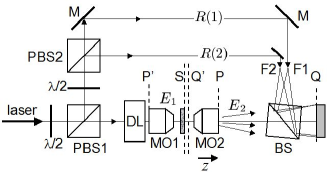
Figure 1: Experimental setup. ${E}_{1}$: incoming field; $E_{2}$: outgoing field; $R(1)$, $R(2)$: reference fields of polarisation $p$=1 and $p$=2; PBS1, PBS2: polarized beam splitters; $\lambda$/2: half wave plate to control $E_{1}$, $R(1)$ and $R(2)$ respective power; BS: beam splitter; M: mirror; DL: diffusing liquid; MO1 and MO2: microscope objectives; Q, Q’: camera plane, and camera conjugate plane with respect to MO2; S: sample outgoing plane. P’ and P: MO1 and MO2 pupil planes.

Figure 1 shows the setup we used to study the open channels by measuring $E_{2}(x,y,t,p)$ and by calculating $C_{2}$ by :

$$C_{2}(t,t^{\prime}) = \frac{\sum_{x,y,p}E_{2}(x,y,t,p)E_{2}^{*}(x,y,t^{\prime},p)}{\sum_{x,y,p}|E_{2}(x,y,t,p)|^{2}}$$ (5)

The setup consists of a Mach-Zehnder off-axis interferometer with two orthogonally polarized reference beams. The light emitted by a $\lambda=532\ \rm nm$, 70 mW laser is split into a reference and an object field using a polarizing beam splitter (PBS1). The studied sample is a ZnO powder slab with thickness $l=22\ \mu\rm m\pm 7\ \mu\rm m$ deposited on a microscope cover slide. In order to maximize the collection of both input and output modes, the sample is positioned between two microscope objectives: MO1 (${\rm NA=0.9}$ air, x60) in the powder side, and MO2 (${\rm NA=1.4}$ oil, x60) in the cover slide side.

A tank (1.5 cm thick) filled with viscous diffusing liquid (glycerol + concentrated milk) is positioned in front of MO1 to randomize the illumination structure in both time and space. The incoming field $E_{1}$ is therefore randomly distributed over all the incoming modes and varies in time. Thus, considering $\left|t-t^{\prime}\right|>100\ \rm ms$, the fields $E_{1}(t)$ and $E_{1}(t^{\prime})$ are uncorrelated.

Measurement of the outgoing field $E_{2}$ is holographically performed. The two orthogonally polarized reference beams $R(p)$ (where $p=1,2$ is polarization) interfere with the outgoing fields $E_{2}(p)$, and the interference pattern $I=\sum_{p=1,2}|R(p)+E_{2}(p)|^{2}$ is recorded on the CCD sensor (10 Hz, $1340\times 1040$ pixels with $\Delta x=6.45\ \mu\rm m$ pitch). This configuration makes it possible to calculate from $I$ the complex amplitudes $E_{2}(p)$ of the outgoing fields along both polarizations $p=1,2$ directions by filtering, in the Fourier space, the desired +1 grating order i.e. $E_{2}(p)R^{*}(p)$ cuche2000spatial .

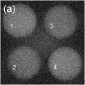
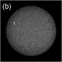
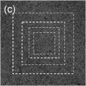
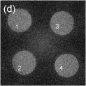
Figure 2: $|{\tilde{H}}|^{2}$ (a,d); $\times 2$ zoom of $|{\tilde{H}}|^{2}$ near zone 1 (b); $|E_{2}R^{*}|^{2}$ calculated by Eq. 6 for $p=1$ (c). In (c), the dashed squares of size $M=$724, 512, 362 and 256 pixels illustrate the ability to select different zones of the sample to calculate $\langle|C_{2}|^{2}\rangle$. Images are obtained with ZnO sample (a-c), and without (d).

The Fourier spacial filtering is illustrated by Fig. 2. The $1340\times 1040$ holograms were cropped to $1024\times 1024$ (the imaged area is therefore $L=77\ \mu\rm m$) and two frames holograms $H$ were calculated from successive frames: $H(t_{2n})=I(t_{2n})-I(t_{2n+1})$. The Fourier hologram $\tilde{H}(k_{x},k_{y})={\rm FFT}\left[H\left(x,y\right)\right]$ (where ${\rm FFT}$ is the Fast Fourier transform) is then calculated. $|\tilde{H}|^{2}$ is displayed on Fig. 2(a). Four bright circular regions can be observed. They correspond to the reconstructed image of the MO2 pupil. Reconstruction is made with +1 grating order $E_{2}(p)R^{*}(p)$ for $p=1$ (zone 1), and $p=2$ (zone 2), and to the -1 grating order $E^{*}_{2}(p)R(p)$ for $p=2$ (zone 3) and $p=1$ (zone 4). Because the calculations are made with two frames hologram, the zero order terms $|R(p)|^{2}$ cancel, and are not visible on Fig. 2(a).

Note that the angular tilt of the beam splitter BS as well as the source point positions $F_{1}$ and $F_{2}$ (see Fig. 1) have been chosen so that the four regions in Fig. 2(a) do not overlap, and have sharp edges verrier2015holographic . From Fig. 2(a), we have selected the desired +1 grating orders $E_{2}R^{*}$ by cropping zone 1 and zone 2 (for $p=1$ and 2) and by taking the inverse Fourier transform of the cropped zones:

$$E_{2}R^{*}(x,y,p)={\rm FFT}^{-1}\rm{C}_{p}\left[\tilde{H}(k_{x},k_{y},p)\right]$$ (6)

where $\rm{C}_{p}$ is the crop operator for polarisation $p$.

Since $R(p)$ is roughly constant with the position $x,y$, the correlations $C_{2}(t,t^{\prime})$ can be then calculated by replacing $E_{2}(x,y,p,t)$ by $[E_{2}R^{*}](x,y,p,t)$ in Eq. 5. The statistical average $\langle|C_{2}|^{2}\rangle$ was obtained by first recording the sequences of 150 camera frames: $I(t_{0})...I(t_{149})$, at times: $t_{n}=n\Delta t$ and $\Delta t=100$ ms, yielding 75 hologram: $H(t_{0}),H(t_{2})...H(t_{148})$, which were used to calculate $[E_{2}R^{*}](x,y,p,t_{2n})$ and $C_{2}(t_{2n},t_{2n^{\prime}})$, and then by averaging $|C_{2}(t_{2n},t_{2n^{\prime}})|^{2}$ for all couple of times $t_{2n},t_{2n^{\prime}}$ with $|n-n^{\prime}|>5$ and $n,n^{\prime}=0..74$.

Because of experimental defects, $|R(p)|$ varies slightly with position. This affects the calculation of $C_{2}(t,t^{\prime})$ and $\langle|C_{2}|^{2}\rangle$. In order to account for this effect, we measured $|R(x,y,p)|$ from our stack of holographic data and we calculated $C_{2}(t,t^{\prime})$ with $[E_{2}R^{*}](x,y,p,t)/|R(x,y,p)|$. This correction is about 10% for $\langle|C_{2}|^{2}\rangle$.

III Number of geometrical modes $N^{\prime}_{g}$

Figure 2 (d) displays the hologram $|\tilde{H}|^{2}$ we got without sample. $|\tilde{H}|^{2}$ exhibits four bright circular zones that are smaller in diameter than with the sample (Fig.2(a)). These circles correspond to the MO1 pupil located in the plane P’ that appears sharp in the plane P, because MO1 and MO2 form an afocal optical system. There is thus no field out of the MO1 collection angle, and the number of geometrical mode $N^{\prime}g$ must be calculated with MO1 numerical aperture NA=0.9.

We must notice that $N^{\prime}_{g}$ is a little bit smaller than the number of pixels of zones 1 and 2 in Fig. 2 (d). Similarly $N_{g}$ is a little bit smaller than the number pixels of zones 1 and 2 in Fig. 2 (a), but the difference is larger, because the brightness within the pupil decreases noticeably near the pupil edge. This means that the reconstructed field within the pupil is random from one pixel to the next.

We used this property to calculate $N_{g}$ and $N^{\prime}_{g}$. We measured the averaged intensities $\langle|{\tilde{H}|^{2}}\rangle$ for each pixels of zone 1 and 2, and we used this information to calculate by Monte Carlo the residual correlation $\langle|C_{2}|^{2}\rangle$ that is expected for pupils fields random in space and time. The number of mode $N_{g}$ and $N^{\prime}_{g}$ we got by this way, with and without sample, agree within a few per cent with $2\pi[\textrm{NA}]^{2}L^{2}/\lambda^{2}$ with NA=1.4 and 0.9.

References

• [1] E. Cuche, P. Marquet, and C. Depeursinge. Spatial filtering for zero-order and twin-image elimination in digital off-axis holography. Appl. Opt., 39, 4070-4075, 2000.
• [2] N. Verrier, D. Alexandre, G. Tessier, and M. Gross. Holographic microscopy reconstruction in both object and image half-spaces with an undistorted three-dimensional grid. Appl. Opt., 54, 4672-4677, 2015.