Equilibrium Surface Current and Role of U(1) Symmetry:
sum rule and surface perturbations

Abstract

We discuss effects of surface perturbations on equilibrium surface currents which contribute to orbital magnetization and orbital angular momentum in systems without time reversal symmetry. We show that, in a U(1) particle number conserving system, disorder and other perturbations at a surface do not affect the equilibrium surface current and corresponding orbital magnetization due to a sum rule which is analogous to Luttinger’s theorem. On the other hand, for a superfluid, the sum rule is no longer applicable and hence the surface mass current and corresponding orbital angular momentum can depend on details of a surface.

I introduction

The orbital magnetization (OM) and orbital angular momentum (OAM) are one of the most fundamental physical quantities in condensed matter physics, which arise in systems without time reversal symmetry due to equilibrium circulating currents. In a continuum (non-lattice) system which does not break translational symmetry in bulk regions, an equilibrium circulating current flows only near its boundary. While in a lattice system, a circulating current is also possible around each atom in addition to a surface current. In spite of their physical importance, however, OM/OAM and associated equilibrium surface currents are not well understood. Indeed, the OM arising from surface currents are usually not taken into account but only locally circulating currents around atoms are included, when one calculates total magnetization of a system in the density functional theory Martin (2004). This would be partly because it is difficult to appropriately treat surface currents theoretically and also effects of surface currents on the total magnetization are expected to be small in conventional ferromagnets such as Fe and Ni.

However, contributions of surface currents to OM/OAM would become important in several interesting systems such as topological insulators/superconductors without time reversal symmetry and fractional quantum Hall systems where there are chiral edge modes Hasan and Kane (2010); Qi and Zhang (2011); Wen (2004). In the last decade, many theoretical studies for OM have been proposed for band insulators and metals including topological systems, and they give a beautiful formula for calculating OM. Gat and Avron (2003a, b); Xiao et al. (2005); Thonhauser et al. (2005); Ceresoli et al. (2006); Shi et al. (2007); Resta (2010); Thonhauser (2011); Xiao et al. (2010); Matsumoto and Murakami (2011); Chen and Lee (2011, 2012). This formula involves only the Bloch wavefunctions which are bulk properties of a system, and hence, the OM and associated surface currents can be regarded as bulk quantities. These results are in good agreement with our general expectations that magnetism is a bulk property which is independent of surface details in real materials. Conceptually, they can be thought as a nice realization of the bulk-surface correspondence in a general sense that bulk properties are determined by surface physics and vice versa. At the same time, however, one may naively expect that surface currents could be affected by perturbations near surfaces which should exist in real materials, such as surface disorder, deformation of Wannier functions, local inversion symmetry breaking, weak screening of the Coulomb interaction, and so on.

A partial answer to this fundamental question can be obtained by following the derivations of the formula for OM. The formula has been derived in three different ways; (i) direct calculations of circulating currents for trivial band insulators in the presence of boundaries Thonhauser et al. (2005); Ceresoli et al. (2006), (ii) semi-classical wavepacket approximations  Xiao et al. (2005, 2010); Matsumoto and Murakami (2011), and (iii) taking derivative of free energy with respect to magnetic fields under the periodic boundary condition  Shi et al. (2007); Chen and Lee (2011). Following the derivation (i), one could find that the surface currents are independent of details of the boundaries when the ground state is a simple band insulator. Based on this, it was argued that effects of surface perturbations on OM in such simple insulators are irrelevant Chen and Lee (2012). Although the discussion presented in the derivation (i) cannot be applied to other systems, the same formula was obtained by the derivations (ii) and (iii). The surface currents are found to be independent of gradient of surface potentials within the semi-classical wavepacket approximations in the derivation (ii). In this approximation, however, the length scale of surface potentials should be much longer than the wavepacket size. In the derivation (iii), although the OM is given as a bulk quantity by its definition for systems with periodic boundary conditions, connections to a surface current which exists in a realistic finite size system are unclear Shi et al. (2007); Chen and Lee (2011). Therefore, in spite of the surprisingly convincing agreements between the three derivations, it is still not clear why the OM and corresponding surface currents are given as bulk quantities which are independent of surface details.

In contrast to non-superconducting systems discussed above, surface perturbations do become relevant for OAM in chiral superfluids which break time reversal symmetry. The OAM in chiral superfluids has been a long-standing issue and attracting much interest since the discovery of ³He A-phase  Leggett (1975); Vollhart and Wölfle (1990); Volovik (2003); Leggett (2006); Ishikawa et al. (1980); Mermin and Muzikar (1980); Kita (1998); Goryo (1998); Furusaki et al. (2001); Stone and Roy (2004); Mizushima et al. (2008); Sauls (2011); Bradlyn et al. (2012); Shitade and Kimura (2014); Hoyos et al. (2014); Tsutsumi (2014); Volovik (2015); Tada et al. (2015); Huang et al. (2014). Effects of surface roughness have been studied in the context of ³He A-phase and Sr₂RuO₄  Mackenzie and Maeno (2003); Maeno et al. (2012), and it was theoretically argued that the surface mass currents and resulting OAM in chiral superfluids depend on surface roughness in weak coupling regions Sauls (2011); Ashby and Kallin (2009); Nagato et al. (2011). In case of domain walls between chiral BCS superfluids with opposite chiralities, the boundary currents strongly depend on difference in U(1) phases of order parameters Tsutsumi (2014); Volovik (2015). Besides, when the surface is sharp, net surface currents vanish for higher order pairing states such as $d+id,f+if$-wave BCS superfluids due to hidden depairing effects which exist even for clean surfaces Tada et al. (2015); Huang et al. (2014). These results suggest that, in contrast to U(1) symmetric systems, surface currents and OAM in superfluids with broken time reversal symmetry depend on surface details and are not bulk quantities. However, physical origins of the reduction of the surface currents and difference between the superfluids and U(1) symmetric systems have not been well understood. Besides, while surface perturbations are known to be relevant in the weak coupling BCS states where Cooper pairs are extended in space, they have not been discussed so far for the strong coupling BEC states where Cooper pairs are strongly bounded Read and Green (2000). For such tightly bounded pairing states, one may naively expect that the surface currents are robust against surface perturbations.

In this paper, in order to clarify the different behaviors of the surface currents and corresponding OM/OAM in systems with or without U(1) symmetry, we discuss effects of surface perturbations from a general point of view. Based on a sum rule argument which is analogous to Luttinger’s theorem  Luttinger (1960); Luttinger and Ward (1960); Yamanaka et al. (1997); Oshikawa (2000); Dzyaloshinskii (2003) and numerical calculations, we show that surface currents are robust against surface perturbations in general U(1) symmetric systems. On the other hand, for superfluids without time reversal symmetry, the sum rule is no longer applicable and surface currents can depend on surface perturbations such as surface roughness. Especially, it is shown that surface currents are suppressed in chiral superfluids on a lattice even for strong coupling BEC states.

This paper organizes as follows. In Sec. II, we discuss surface currents in U(1) symmetric systems. We show a sum rule for the surface current in general systems and confirm it by numerical calculations for a concrete model. The OM formula is revisited based on the sum rule argument. Then, surface currents in U(1) broken systems are examined in Sec III. Finally, we summarize this paper in Sec. IV

II system with U(1) symmetry

II.1 sum rule argument

In this section, we discuss surface currents in U(1) symmetric systems. For simplicity, we consider 2-dimensional lattice models whose size is $N_{x}\times N_{y}$ with the open boundary condition for $x$-direction and the periodic boundary condition for $y$-direction as shown in Fig. 1.

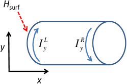
Figure 1: Schematic picture of the two-dimensional cylinder system.

Our argument holds also for continuum models as discussed in Appendix A. We assume that there is no time reversal symmetry and there can exist equilibrium surface currents for the models considered. Our Hamiltonian reads in general

$$H =\sum c^{\dagger}_{xl}(k_{y})K_{xl,x^{\prime}l^{\prime}}(k_{y})c_{x^{\prime}l^{\prime}}(k_{y})+H_{\rm int}+H_{\rm surf}$$ (1)

where $c_{xl}(k_{y})$ is an annihilation operator of electrons at position $x$, with wavenumber along $y$-direction $k_{y}$ and other quantum number $l$ such as orbitals and spins. The matrix $\hat{K}$ describes one-particle Hamiltonian. We assume that the interaction $H_{\rm int}$ is simply short-range density-density interactions or on-site interactions so that it commutes with the total particle density operator, $[n_{i},H_{\rm int}]=0$. $H_{\rm surf}$ is the surface perturbation term which is finite only near the surface and zero otherwise, and is also assumed to satisfy $[n_{i},H_{\rm sruf}]=0$. Therefore, the U(1) current operator is simply given by the kinetic term only through the continuity equation in the present study.

In this geometry, the equilibrium surface current at the left (right) surface is given by

$$I_{y}^{L(R)}=\frac{1}{N_{y}}\sum_{xx^{\prime}\in S_{L}(S_{R})}v_{y;xl,x^{\prime}l^{\prime}}(k_{y})\langle c^{\dagger}_{xl}(k_{y})c_{x^{\prime}l^{\prime}}(k_{y})\rangle,$$ (2)

in unit of the electron charge $e$. $S_{L(R)}$ is a region only near the left (right) surface whose width is much smaller than the system width $N_{x}$. Since effects of a surface should not propagate deep into bulk regions, we can define such regions in general systems com (a). $\hat{v}_{y}$ is a velocity matrix given by $\hat{v}_{y}(k_{y})=\partial\hat{K}(k_{y})/\partial k_{y}$. In the absence of $H_{\rm surf}$ it is obvious that $I_{y}^{\rm tot}\equiv I_{y}^{L}+I_{y}^{R}=0$ under a natural assumption that the Hamiltonian (1) has inversion symmetry in the $x$-direction, $x\leftrightarrow-x$. Since current density which contributes to the surface current is localized only around the surface and it vanishes in bulk regions out of $S_{L,R}$ com (a), the total surface current $I_{y}^{\rm tot}$ is written as

$$I_{y}^{\rm tot} =\frac{1}{N_{y}}\sum_{xx^{\prime}\in\mbox{all sites}}v_{y;xl,x^{\prime}l^{\prime}}(k_{y})\langle c^{\dagger}_{xl}(k_{y})c_{x^{\prime}l^{\prime}}(k_{y})\rangle$$

$$=\frac{1}{N_{y}}\sum_{k_{y}}{\rm tr}\bigl{[}\hat{v}_{y}(k_{y})\hat{G}(k_{y},i\omega)e^{i\omega 0^{+}}\bigr{]}.$$ (3)

Here, $\hat{G}(k)=\hat{G}(k_{y},i\omega)=-\langle\langle c(k_{y})c^{\dagger}(k_{y})\rangle\rangle(i\omega)$ is the matrix Matsubara Green’s function, and trace describes summation over all the indices, $x,l$ and $\omega$. We note that, although off diagonal elements become finite if the system breaks some symmetries together with time reversal symmetry such as spin rotation symmetry in a ferromagnetic state, our discussion holds in a parallel way by introducing order parameters into $\hat{G}$ and modifying the definition of $\hat{v}_{y}$ appropriately. For example, if the translational symmetry along the $y$-direction is preserved, only possible off diagonal elements in the Green’s function are of the form $\langle c_{x^{\prime}l^{\prime}}(k_{y})c^{\dagger}_{xl}(k_{y})\rangle$ which have already been included in the above expression. If the translational symmetry along the $y$-direction is broken, although off diagonal elements with different momenta $k_{y}$ and $k_{y}+Q_{y}$ with an ordering vector $Q_{y}$ become finite, Eq. (3) is still valid after modifying $\hat{v}_{y}(k_{y})$ to $\tilde{v}_{y}(k_{y})={\rm diag}(\hat{v}_{y}(k_{y}),\hat{v}_{y}(k_{y}+Q_{y}))$ where $k_{y}$ belongs to the reduced Brillouin zone.

Now we turn on $H_{\rm surf}$ which is finite only near the left surface and zero in all the other regions including the right surface. Our fundamental assumption is that $I_{y}^{R}$ is unchanged by the left surface perturbation $H_{\rm surf}$ as long as the width of the cylinder is large enough, which means that if $I_{y}^{\rm tot}$ changes, it is totally attributed to change in $I_{y}^{L}$. We also assume that $H_{\rm surf}$ is translationally symmetric along the surface. In case of surface disorder, $H_{\rm surf}$ is still translationally symmetric on average, for which the disorder-averaged Green’s function is diagonal with respect to $k_{y}$. Then, all the effects of such perturbations in one-particle quantities can be incorporated into the (averaged) selfenergy matrix $\hat{\Sigma}(k)$. Effects of $H_{\rm int}$ are also described by the selfenergy, and if the system is in broken symmetry states, we include the corresponding order parameter matrix in $\hat{\Sigma}(k)$. The Green’s function $\hat{G}(k)$ is now written as a matrix inverse of $[i\omega-\hat{K}(k_{y})-\hat{\Sigma}(k)]$. Therefore,

$$I_{y}^{\rm tot} =\frac{1}{N_{y}}\sum_{k_{y}}{\rm tr}\Bigl{[}\frac{\partial\hat{K}(k_{y})}{\partial k_{y}}\hat{G}(k)\Bigr{]}$$

$$=-\frac{1}{N_{y}}\sum_{k_{y}}{\rm tr}\Bigl{[}\frac{\partial\hat{G}^{-1}}{\partial k_{y}}\hat{G}\Bigr{]}-\frac{1}{N_{y}}\sum_{k_{y}}{\rm tr}\Bigl{[}\frac{\partial\hat{\Sigma}}{\partial k_{y}}\hat{G}\Bigr{]}$$

$$=-\frac{1}{2\pi}{\rm tr}\log\Bigl{[}\frac{\hat{G}(k_{y}=\pi,i\omega)}{\hat{G}(k_{y}=-\pi,i\omega)}\Bigr{]}-\frac{1}{N_{y}}\sum_{k_{y}}{\rm tr}\Bigl{[}\frac{\partial\hat{\Sigma}}{\partial k_{y}}\hat{G}\Bigr{]}.$$ (4)

It is clear that the first term vanishes. (If the translational symmetry is broken, $k_{y}=\pm\pi$ should be replaced by appropriate boundary $k$-vectors of the reduced Brillouin zone.) Second term also vanishes because of the Luttinger-Ward identity Luttinger (1960); Luttinger and Ward (1960); Dzyaloshinskii (2003); com (b),

$$\frac{1}{N_{y}}\sum_{k_{y}}{\rm tr}\Bigl{[}\frac{\partial\hat{\Sigma}(k)}{\partial k_{y}}\hat{G}(k)\Bigr{]}=0.$$ (5)

Although the Luttinger-Ward identity may be violated in Mott insulators  Rosch (2007); Dave et al. (2013), it holds in general gapless/gapped Fermi liquids where there is no zero (pole) in the Green’s function (selfenergy), and also in weakly disordered systems com (b). As long as the Luttinger-Ward identity is satisfied, $I_{y}^{\rm tot}=I_{y}^{L}+I_{y}^{R}=0$ even in the presence of the perturbations around the left surface, which means that $I_{y}^{L}$ is unchanged although the current density at each site could be affected by $H_{\rm surf}$.

There is a nice analogy between the conservation of surface currents in the presence of surface perturbations and the well known conservation law, the Luttinger’s theorem Luttinger (1960); Luttinger and Ward (1960); Yamanaka et al. (1997); Oshikawa (2000); Dzyaloshinskii (2003). The Luttinger’s theorem claims that, though shape of a Fermi surface can be changed by interactions, its total volume is unchanged. Here, although a real space profile of U(1) surface current density $j_{i}$ can be modified by the surface perturbations, its sum around the surface $I=\sum_{i\in{\rm surf}}j_{i}$ is unchanged. In this view point, the conservation of the U(1) surface current in the presence of surface perturbations is understood as a result of non-trivial cancellations of changes in $j_{i}$ at each site. This sum rule argues that surface currents and corresponding OM are bulk quantities which are independent of surface details as suggested in the modern theories on OM Xiao et al. (2005); Thonhauser et al. (2005); Ceresoli et al. (2006); Shi et al. (2007); Resta (2010); Thonhauser (2011); Xiao et al. (2010); Matsumoto and Murakami (2011); Chen and Lee (2011, 2012), and this supports existence of the bulk-surface correspondence for these quantities. We note that, the sum rule is useful not only for developments in understanding fundamental aspects of surface currents, but also for practical calculations of them. Although realistic surface potentials would be complicated in general, one can use a particular surface potential which is suitable for computing them, such as a hard wall potential and a sufficiently smooth potential. The sum rule guarantees that the calculation results of the surface current and OM are independent of the potential used. Indeed, the known formula for OM can be reproduced by calculating surface current contributions and also contributions from locally circulating currents under a sufficiently smooth surface potential, as will be discussed in Sec. II.4.

Up to now, we have not considered external or spontaneously generated magnetic fields. In the presence of an applied magnetic field parallel to the $z$-direction, the hopping integrals acquire phase factors corresponding to the flux configuration by the Peierls substitution, and the Brillouin zone is reduced to a magnetic Brillouin zone. Even in this case, by appropriately modifying the definition of $\hat{v}(k_{y})$, we can still derive a sum rule for a surface current in the same way. The surface current under a magnetic field for a time reversal symmetric system is related to the Landau diamagnetism. It has been known that “bulk approaches” and “surface approaches” are equivalent for the Landau diamagnetism; it can be calculated either by derivative of free energy with respect to the magnetic field under periodic boundary conditions Landau (1930); Peierls (1933); Fukuyama (1971) or by computing a surface current in the presence of boundaries  Kubo (1964); Ohtaka and Moriya (1973); Ishikawa and Fukuyama (1999), and these two approaches consistently give the same results. Experimentally, the skipping orbits which would be responsible for the surface current have been observed in surface impedance measurements for many metals  Nee et al. (1968); Abrikosov (1988). Our sum rule argument would give a new understanding on the known equivalence between the two theoretical approaches.

Finally, it is noted that, the sum rule can hold since the U(1) charges of the electrons are the well defined unique value $e$ in the systems with U(1) symmetry. If U(1) symmetry is absent, however, particle sectors with charge $+e$ and hole sectors with $-e$ are mixed and the surface currents will not generally be conserved, as will be discussed in Sec. III.

II.2 Bloch-Bohm’s theorem

In this section, we discuss relations of our sum rule to the Bloch-Bohm’s theorem. The theorem states that net current should vanish in the ground states Bohm (1949); Vignale (1995); Ohashi and Momoi (1996); Kusama and Ohashi (1999). Here, we reexamine this theorem and point out that (i) it does not hold when surface currents are concerned and (ii) it needs some modifications when spontaneous symmetry breaking is involved even for currents running in bulk regions.

We consider a general Hamiltonian as in Eq. (1) without symmetry breaking fields in a finite size cylinder $L\times L$ where open (periodic) boundary condition is imposed for $x(y)$-direction, and denote the ground state wavefunction as $|0_{L}\rangle$. Since the system size is finite, there is no spontaneous symmetry breaking and the ground state wavefunction preserves the symmetries of the Hamiltonian including the time reversal symmetry if it is contained in $H$. When the Hamiltonian has time reversal symmetry, it is trivial that the total current $I^{\rm tot}_{y}$ vanishes because it is odd under the time reversal symmetry. In the following, we mainly discuss $H$ with time reversal symmetry and $H$ without time reversal symmetry will be touched on briefly. For time reversal symmetric $H$, we introduce external fields $\lambda H_{\rm ex}=\lambda\sum\Delta_{il,jl^{\prime}}c^{\dagger}_{il}c_{jl^{\prime}}$ which break time reversal symmetry by assuming that the state $|0_{L}\rangle$ of $H$ has corresponding instability, where $\lambda$ is a dimensionless constant which should be taken as $\lambda\rightarrow 0$ in the end. Although we focus on U(1) symmetric external fields in this section, effects of U(1) symmetry breaking fields will be discussed in Sec. III.

Following Bohm (1949), we consider a variational state $|\theta_{L,\lambda}\rangle=U_{\theta}|0_{L,\lambda}\rangle$ where $|0_{L,\lambda}\rangle$ is the ground state of $H_{\lambda}=H+\lambda H_{\rm ex}$. The unitary operator is defined as $U_{\theta}=\exp[i\theta\sum_{j}yn_{j}]$ Lieb et al. (1961); Yamanaka et al. (1997); Oshikawa (2000), and $\theta=2\pi n/L,(n=0,\pm 1,\cdots)$ is required so that $U_{\theta}$ is a well-defined operator. This requirement can easily be understood from the first quantization form of $U_{\theta}$; the twist operator for the wavefunction $\Psi(\mbox{\boldmath$r$}_{1},\cdots,\mbox{\boldmath$r$}_{N})=\Psi(\mbox{\boldmath$r$}_{1}+L,\cdots,\mbox{\boldmath$r$}_{N}+L)$ is given by $U_{\theta}=\exp[i\theta\sum_{j}y_{j}]$. In order for $\Psi^{\prime}(\mbox{\boldmath$r$}_{1},\cdots,\mbox{\boldmath$r$}_{N})=(U_{\theta}\Psi)(\mbox{\boldmath$r$}_{1},\cdots,\mbox{\boldmath$r$}_{N})$ to satisfy the periodic boundary condition, $\theta=2\pi n/L$ is needed. If $\theta$ were not an integer multiple of $2\pi/L$, the wavefunction $(U_{\theta}\Psi)$ is no longer an element of the domain of the Hamiltonian. This is essentially comes from the well-known fact that position operators cannot be well-defined on a torus, although it is sometimes missed even by experts Carruthers and Nieto (1968). Similarly in the second quantization formalism, $c_{jl}^{\prime}=U^{\dagger}_{\theta}c_{j}U_{\theta}=e^{-i\theta j}c_{jl}$ obeys the periodic boundary condition when $\theta=2\pi n/L$ is satisfied. Although this fundamental point has been missing in most of the previous studies concerning Bloch-Bohm’s theorem, this is important especially for discussing possible net surface currents.

We then evaluate energy difference between $|\theta_{L,\lambda}\rangle$ and $|0_{L,\lambda}\rangle$,

$$\delta E_{L,\lambda} =\langle\theta_{L,\lambda}|H_{\lambda}|\theta_{L,\lambda}\rangle-\langle 0_{L,\lambda}|H_{\lambda}|0_{L,\lambda}\rangle$$

$$=\sum(\cos[\theta(y_{i}-y_{j})]-1)\langle 0_{L,\lambda}|c_{il}^{\dagger}K_{il,jl^{\prime}}c_{jl^{\prime}}|0_{L,\lambda}\rangle$$

$$\quad+\lambda\sum(\cos[\theta(y_{i}-y_{j})]-1)\langle 0_{L,\lambda}|c_{il}^{\dagger}\Delta_{il,jl^{\prime}}c_{jl^{\prime}}|0_{L,\lambda}\rangle$$

$$\quad+\sum i\sin[\theta(y_{i}-y_{j})]\langle 0_{L,\lambda}|c_{il}^{\dagger}K_{il,jl^{\prime}}c_{jl^{\prime}}|0_{L,\lambda}\rangle$$

$$\quad+\lambda\sum i\sin[\theta(y_{i}-y_{j})]\langle 0_{L,\lambda}|c_{il}^{\dagger}\Delta_{il,jl^{\prime}}c_{jl^{\prime}}|0_{L,\lambda}\rangle.$$ (6)

It is well known that the Lieb-Schultz-Mattis twist operator $U_{\theta}$ is not helpful for higher dimensions other than one-dimension, in order to construct a variational state with low energy excitations. Indeed, since $\cos[\theta(y_{i}-y_{j})]-1\sim O(1/L^{2})$ in the present model with a finite hopping range $l_{t}$ which is much shorter than $L$, the $\cos[\theta(y_{i}-y_{j})]$-terms are obviously $O(1)$ for large $L$ limit. In general $d$-dimensional system of an isotropic size $L$ for all directions, these terms are $O(L^{d-2})$. Therefore, the $\sin[\theta(y_{i}-y_{j})]$-terms could become dominant for large $L$, if at least one of them is of order $L$ or larger, namely $\sum i\sin[\theta(y_{i}-y_{j})]\langle c^{\dagger}_{i}Kc_{j}\rangle\sim O(L)$ or $\sum i\sin[\theta(y_{i}-y_{j})]\langle c^{\dagger}_{i}\Delta c_{j}\rangle\sim O(L)$. By expanding $\sin[\cdots]$, we see that one of the $\sin[\cdots]$-terms is simply the total current running in the whole system, $\theta\langle 0_{L,\lambda}|\sum_{i}j_{yi}|0_{L,\lambda}\rangle$ in the leading order of $\theta\ll 1$, where $j_{yi}$ is current density. The original Bloch-Bohm’s theorem states that, since we can choose either $\theta=2\pi/L$ or $\theta=-2\pi/L$, in order for $\delta E_{L,\lambda}$ to be non-negative, $\langle 0_{L,\lambda}|\sum_{i}j_{yi}|0_{L,\lambda}\rangle$ must be zero in the thermodynamic limit $L\rightarrow\infty$. However, the Bloch-Bohm’s argument is based on an implicit assumption that the expectation value of the total current is $\langle\sum_{i}j_{yi}\rangle\sim O(L^{2})$, and also the other sin-term is negligible, $\sum i(y_{i}-y_{j})\langle c^{\dagger}_{i}\Delta c_{j}\rangle\sim o(L)$. At the same tiem, we also should pay attention to the $\cos[\cdots]$-terms which are $O(1)$. In the case of surface currents without any current density in the bulk, contributions only come from the surface regions $S_{L,R}\sim O(1)$, and therefore $\theta\langle\sum_{i}j_{yi}\rangle\sim(1/L)\times L=O(1)$ and it becomes the same order as the $\cos$-terms. In $d$-dimensional systems, $\theta\langle\sum_{i}j_{yi}\rangle\sim(1/L)\times L^{d-1}=O(L^{d-2})$ and it competes with the $\cos$-terms as well, for which we cannot immediately conclude that finite $\langle 0_{L,\lambda}|\sum_{i}j_{yi}|0_{L,\lambda}\rangle\sim O(L^{d-1})$ contradicts with $\delta E_{L,\lambda}$. Hence, the Bloch-Bohm’s argument is not applicable when surface currents are concerned, although it might give an upper bound for the net surface currents. On the other hand, the sum rule argument in the previous section claims that surface currents should be exactly canceled between opposite surfaces in a cylinder.

The above observation is applicable either with or without the symmetry breaking fields. In the following, we discuss some subtleties related to the external fields and the thermodynamic limit, which have also been overlooked in the previous studies. Here, we focus on possibilities of total currents of order $L^{2}$ ($L^{d}$ in $d$-dimensions), which are bulk currents but not surface currents. Firstly, we consider a case where $H$ itself does not have time-reversal symmetry without symmetry breaking fields, although such a Hamiltonian would be artificial. In this case, we could keep $L$ to be some large but finite values, so that the total current term becomes dominant in $\delta E_{L,\lambda=0}$. Then, we can safely apply the original Bloch-Bohm’s argument to conclude that total current of order $L^{2}$ must vanish for sufficiently large $L$.

However, if we include the symmetry breaking fields for time reversal symmetric $H$, we have extra terms in $\delta E_{L,\lambda}$ arising from $\lambda H_{\rm ex}$ and the resulting $O(L)$ term in $\delta E_{L,\lambda}$ is not determined by the total current only, $\delta E_{L,\lambda}\sim(\pm 2\pi/L)\langle\sum[j_{yi}+\lambda(\cdots)]\rangle$ where $\lambda(\cdots)$ represents $\lambda i(y_{i}-y_{j})c^{\dagger}_{i}\Delta c_{j}$. At this point, what is forbidden by the Bloch-Blohm’s argument is that the above expectation value is some finite value of order $L^{2}$ for large $L$. We do not know, however, which contribution in the bracket becomes dominant for given $L,\lambda$, although the second term may be smaller for sufficiently small $\lambda$. Furthermore, since we are interested in the spontaneously symmetry broken states, we should take the limit of vanishing external fields $\lambda\rightarrow 0$. When the system is defined on $x,y=-L/2+1,\cdots,L/2$ with an even $L$, we consider

$$\delta\varepsilon_{n}\equiv\lim_{\lambda\downarrow 0}\lim_{L\uparrow\infty}\frac{\delta E_{L,\lambda}}{L^{n}}.$$ (7)

The contribution arising from $\lambda H_{\rm ex}$ will vanish as $\lambda\rightarrow 0$ due to the prefactor $\lambda$ in front of $H_{\rm ex}$, as long as the expectation value $\lim_{L\uparrow\infty}\sum(2\pi/L^{n+1})\langle 0_{L,\lambda}|c^{\dagger}\Delta c|0_{L,\lambda}\rangle$ is not singular at $\lambda=0$. Because we have assumed that time reversal symmetry is broken and the corresponding order parameter is finite in the thermodynamic limit, this term should be some constant which is independent of $\lambda$ in the limit $\lambda\rightarrow 0$, and therefore we can safely take the limit. It is noted that difference in the thermodynamic energy density $\delta\varepsilon_{2}$ vanishes in this limit, while $\delta\varepsilon_{1}$ can be negative if the total surface current per volume is $O(1)$ for finite $L$ and is non-zero after taking the limit. However, we should be careful about meaning of the possible non-zero $\delta\varepsilon_{1}$. In the thermodynamic limit, quantum states for fixed $\lambda$ may be defined as

$$\omega_{0}(\cdot) =\lim_{L\uparrow\infty}\langle 0_{L,\lambda}|\cdot|0_{L,\lambda}\rangle,$$ (8)

$$\omega_{\theta}(\cdot) =\lim_{L\uparrow\infty}\langle\theta_{L,\lambda}|\cdot|\theta_{L,\lambda}\rangle$$ (9)

for local operators Emch (1972). There are some subtleties in the thermodynamic limit, where there is no local operator describing the total current density for the whole system corresponding to $\delta\varepsilon_{1}\sim\langle\sum j_{yi}\rangle/L^{2}$. In this case, the two thermodynamic states $\omega_{0},\omega_{\theta}$ become identical;

$$\omega_{0}(A)=\omega_{\theta}(A)$$ (10)

for any local operator $A$. For example, $\omega_{\theta}(c^{\dagger}_{il}c_{jl^{\prime}})=\lim_{L\uparrow\infty}e^{i\theta(y_{i}-y_{j})}\langle 0_{L,\lambda}|c^{\dagger}_{il}c_{jl^{\prime}}|0_{L,\lambda}\rangle=\omega_{0}(c^{\dagger}_{il}c_{jl^{\prime}})$ because $|y_{i}-y_{j}|<l_{t}$ is finite and $\lim_{L\uparrow\infty}e^{i\theta(y_{i}-y_{j})}=1$. (Note that expectation values of U(1) breaking local operators vanish trivially for both states.) This is true even when the two states are orthogonal for finite $L$, and the two orthogonal states can converge to a single state in the thermodynamic limit.

Such a behavior arises from global nature of the variational state $|\theta_{L,\lambda}\rangle$. The two states $|0_{L,\lambda}\rangle,|\theta_{L,\lambda}\rangle$, are almost identical locally and their difference appears as a sum of these tiny local differences. In the present system, to obtain different states in the thermodynamic limit, we need to restrict the twist only for a finite support such as $D=\{(x,y)|1\leq x-\bar{x},y-\bar{y}\leq L^{\prime}\}$ where $(\bar{x},\bar{y})$ is an arbitrary site. We then define a new variational state $|\theta^{\prime}_{L,\lambda}\rangle=U_{\theta}^{\prime}|0_{L,\lambda}\rangle$, $U_{\theta}^{\prime}=\exp[i\theta^{\prime}\sum^{\prime}y_{j}n_{j}]$ where $\theta^{\prime}=2\pi/L^{\prime}$ and the summation is taken only for the above finite domain $D$ Yamanaka et al. (1997). It is noted that, in order for $U_{\theta}^{\prime}$ to be well-defined, $L^{\prime}$ should be $L/L^{\prime}=$integer. When we take the thermodynamic limit, we keep $L^{\prime}$ constant but increase $L$ only. Nevertheless, we can take $L^{\prime}$ to be much larger than the finite hopping range of the model $l_{t}\ll L^{\prime}$. Then, the energy difference for $\theta^{\prime}=\pm 2\pi/L^{\prime}$ is $\delta E_{L,\lambda}=\pm(2\pi/L^{\prime})\sum^{\prime}\langle 0_{L,\lambda}|j_{yi}+\lambda(\cdots)|0_{L,\lambda}\rangle+O(l_{t}/L^{\prime})$. By taking the limit, the energy difference for $\theta=\pm 2\pi/L^{\prime}$ becomes

$$\lim_{\lambda\downarrow 0}\lim_{L\uparrow\infty}\delta E_{L,\lambda}=\pm\frac{2\pi}{L^{\prime}}\lim_{\lambda\downarrow 0}\lim_{L\uparrow\infty}\langle 0_{L,\lambda}|\sum_{i}^{\prime}j_{yi}|0_{L,\lambda}\rangle+O(L^{\prime 0}),$$ (11)

where the $O(L^{\prime 0})=O(1)$ term come from the cos-term. Note that the first term does not describe total current of the system, but it corresponds to current running within the finite region $D$. Here, we recall that the ground state of $H_{\lambda}$ in the thermodynamic limit is defined so that $\omega_{0}(A^{\dagger}[H_{\lambda},A])\geq 0$ is satisfied for any local operator $A$. If we take $A=U_{\theta}^{\prime}$, this means

$$\lim_{\lambda\downarrow 0}\omega_{0}(U_{\theta}^{\prime\dagger}H_{\lambda}U_{\theta}^{\prime}-H_{\lambda})=\lim_{\lambda\downarrow 0}\lim_{L\uparrow\infty}\delta E_{L,\lambda}\geq 0.$$ (12)

By comparing Eqs. (11) and  (12), we conclude that the current running in the domain $D$ cannot be of order $O(L^{\prime 2})$ for sufficiently large $L^{\prime}\gg l_{t}$. This statement is a bit stronger than the original Bloch-Bohm’s argument, since the position of $D$ characterized by the site $(\bar{x},\bar{y})$ can be arbitrary in the infinite system. Hence, we conclude that there is no macroscopic flow anywhere in a thermodynamic system. We will see that this statement holds for U(1) symmetry broken systems as well in Sec. III. The only remaining possibilities would be locally circulating currents in an atomic scale and surface currents which are of smaller order in $L^{\prime}$ as discussed before.

II.3 numerical simulation

In order to confirm the sum rule argument, we perform numerical calculations of surface currents in a simple toy model defined on a square lattice cylinder. We impose the open (periodic) boundary condition for the $x(y)$-direction. As typical examples of surface perturbations, we investigate effects of surface roughness and surface potentials. We consider the following Hamiltonian

$$H_{\rm AH} =H_{\rm AH0}+H_{\rm surf},$$ (13)

$$H_{\rm AH0} =\sum_{\rm NN}[-tc^{\dagger}_{i1}c_{j1}+tc^{\dagger}_{i2}c_{j2}+t^{\prime}e^{i\theta_{ij}}c^{\dagger}_{i1}c_{j2}+({\rm h.c.})]$$

$$\quad+\sum M[n_{i1}-n_{i2}],$$

$$H_{\rm surf} =\sum V_{il}n_{il},$$

where $e^{i\theta_{i,i\pm\hat{x}}}=\mp i,e^{i\theta_{i,i\pm\hat{y}}}=\pm 1$, and $V_{il}$ is the surface perturbation. This model is a spinless version of the Bernevig-Hughes-Zhang model, and does not have time reversal symmetry Hasan and Kane (2010); Qi and Zhang (2011). In the present calculations, $V_{il}$ is finite only at the left surface sites $i=(x=1,y)$. We study two cases: (i) $V_{i1,2}$ take real random values in $[-V_{0},V_{0}]$ in case of surface roughness, and (ii) $V_{i1,2}$ are constant, $(V_{i1},V_{i2})=(V_{0},0)$, as a particular realization of surface potentials. Since the $t^{\prime}$-term is simply a part of kinetic term which arises from spin-orbit interaction in the original Bernevig-Hughes-Zhang model, the current density operator for the $\mu=x,y$-direction in the present model is given by

$$j_{\mu i} =-it[c^{\dagger}_{i1}c_{i+\hat{\mu}1}-c^{\dagger}_{i+\hat{\mu}1}c_{i1}]+it[c^{\dagger}_{i2}c_{i+\hat{\mu}2}-c^{\dagger}_{i+\hat{\mu}2}c_{i2}]$$

$$\quad+it^{\prime}e^{i\theta_{ii+\hat{\mu}}}[c^{\dagger}_{i1}c_{i+\hat{\mu}2}+c^{\dagger}_{i+\hat{\mu}1}c_{i2}]+({\rm h.c.}).$$ (14)

For simplicity, we fix $(t^{\prime},M)=(0.2t,-3t)$ as an example, and filling is $n=n_{1}+n_{2}=0.7$ for which the system is in a metallic anomalous Hall state. Temperature is fixed at $T=0$. System size is $N_{x}\times N_{y}=80\times 20$ for the case (i), and numerical results are checked for other systems sizes. For the case (ii), with use of Fourier transformation for the $y$-direction, larger system sizes are examined.

In Fig. 2, we show the current densities $j_{yi}$ for the random potential and constant potential at a large $V_{0}=2t\gg t^{\prime}=0.2t$ together with $j_{yi}$ for $V_{0}=0$ (which we denote $j_{yi}^{0}$ hereafter). We see that $j_{xi}$ vanishes everywhere in the system and $I^{R}_{y}$ is unchanged by the left surface potentials. For the random potential, we take a disorder average $\langle j_{yi}\rangle_{\rm av}$ and then take an average of them along the $y$-direction, $(1/N_{y})\sum_{y=1}^{N_{y}}\langle j_{yi}\rangle_{\rm av}$. It is seen that, although there are some small oscillations in the bulk region due to metallicity in the present model, $j_{yi}$ is localized around the surfaces. The current densities are modified from $j_{yi}^{0}$ around the left surface $x=0$. However, we find that, both for the random potential and constant potential, the left surface current $I_{y}^{L}=(1/N_{y})\sum_{i\in{\rm surf}}j_{yi}$ is unchanged from $I_{y}^{0}=(1/N_{y})\sum_{i\in{\rm surf}}j_{yi}^{0}$, which is confirmed for several different system sizes. Conservation of the surface currents were also seen in the previous study for a constant surface potential in an insulating state Chen and Lee (2012). In the case of disorder potential, distribution of $I_{y}^{L}$ for different configurations of the potential is well localized around its mean value $I_{y}^{0}$ as shown in Fig. 3. It is noted that the distribution of $I_{y}^{L}$ gets broader if we introduce inter-orbital random potentials $\sum[V_{i12}c_{i1}^{\dagger}c_{i2}+({\rm h.c.})]$ in addition to the intra-orbital potential (not shown). Although finite size effects become rather large in this case, the average surface current is still unchanged by the surface disorder. We have performed similar calculations for other realizations of surface potentials, and confirmed that the surface current is unchanged by them. These numerical calculations indeed support the sum rule argument in Sec. II.1.

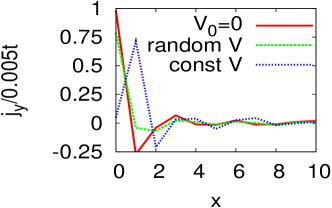
Figure 2: Current density $j_{y}$ near the left surface for $V_{0}=0$ (red), random potential with $V_{0}=2t$ (green), and constant potential with $V_{0}=2t$.

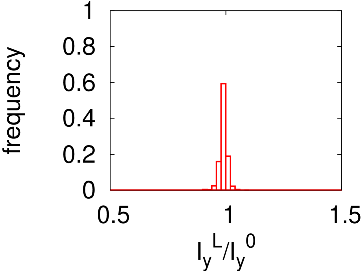
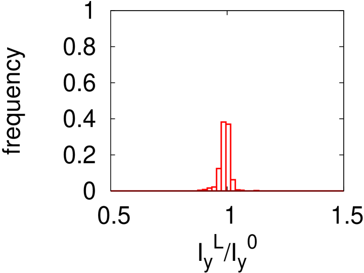
Figure 3: Normalized histogram of $I_{y}^{L}$ for disorder potentials $V_{0}=0.5t$ (left panel) and $V_{0}=2t$ (right panel).

II.4 Revisit of Orbital Magnetization Formula

As mentioned in Sec. II.1, the sum rule is helpful not only for basic understanding of surface currents but also for practical calculations of them. Here, based on an observation of the sum rule, we rederive the formula of orbital magnetization $M$ at $T=0$ Xiao et al. (2005); Thonhauser et al. (2005); Ceresoli et al. (2006); Shi et al. (2007); Resta (2010); Thonhauser (2011); Xiao et al. (2010); Matsumoto and Murakami (2011); Chen and Lee (2011, 2012) for a thermodynamically large but finite size system. We consider a non-interacting model of size $L\times L$ with the periodic boundary condition, whose Hamiltonian is expressed in a Wannier function basis as $H_{0}=\int_{L^{2}}d^{2}x\psi^{\dagger}{\mathcal{K}}\psi=\sum_{ijll^{\prime}}c^{\dagger}_{il}\hat{H}_{0}c_{jl^{\prime}}$. The chemical potential has been included in $H_{0}$. Then, we introduce a confinement potential, $H_{\rm surf}=\sum_{i}V_{i}n_{i}$, which smoothly varies in space and is zero inside a region $l\times l$ while infinitely large outside. The length scales can be taken as

$$a\ll\xi_{V}\ll l\ll L$$ (15)

where $a$ is the lattice constant and $\xi_{V}$ characterizes the spatial variation length of $V$. The system configuration is schematically shown in Fig. 4.

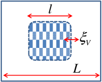
Figure 4: Schematic picture of the system with the confinement potential $V$ which is zero in the shaded region and infinite in the white region. $V$ changes in a length scale $\xi_{V}$ which is much longer than the lattice constant $a$. These length scales satisfy $a\ll\xi_{V}\ll l\ll L$.

Although such a confinement potential would not be a realistic surface potential, the sum rule guarantees that the surface current is equivalent to that with a realistic confinement potential. It is noted that, as long as the length scale of the confinement potential is much shorter than the system size $\xi_{V}\ll l$, the locally circulating current around each atom in the bulk is not affected by the potential.

Generally, the paramagnetic current density in unit of $e$ and orbital magnetization in a finite system with boundaries are given by  Eschrig et al. (1985); Vignale and Rasolt (1987); Higuchi and Hasegawa (1997),

$$\mbox{\boldmath$j$}(\mbox{\boldmath$r$}) =\frac{-i}{2m}\bigl{[}\psi^{\dagger}\nabla\psi-\nabla\psi^{\dagger}\psi\bigr{]},$$ (16)

$$M_{z}\times{\rm vol} =\frac{1}{2}\int_{\rm finite}d^{2}x[\mbox{\boldmath$r$}\times\mbox{\boldmath$j$}(\mbox{\boldmath$r$})]_{z}$$

$$=\frac{1}{2}\sum_{i}\int_{v_{i}}d^{2}x(\mbox{\boldmath$r$}-\mbox{\boldmath$R$}_{i})\times\mbox{\boldmath$j$}(\mbox{\boldmath$r$})|_{z}$$

$$\qquad\qquad+\frac{1}{2}\sum_{i}\mbox{\boldmath$R$}_{i}\times\int_{v_{i}}d^{2}x\mbox{\boldmath$j$}(\mbox{\boldmath$r$})|_{z},$$ (17)

where $v_{i}$ is a unit cell with its center position $\mbox{\boldmath$R$}_{i}$. The first term in $M_{z}$ arises from locally circulating current, while the second term is due to the surface current.

We first consider the surface contribution. In the presence of the smooth confinement potential, derivative expansion in the Wigner representation would be legitimate Volovik (2003); Kubo (1964), where the site index $i$ can be considered as a continuum variable in the length scale $\xi_{V}\gg a$. The Green’s function is approximated up to the lowest order with respect to derivative of the confinement potential by,

$$\hat{G}(\mbox{\boldmath$X$},k) =\hat{G}_{0}\Bigl{[}1+\frac{i}{2}\frac{\partial\hat{G}_{0}^{-1}}{\partial X_{\mu}}\frac{\partial\hat{G}_{0}}{\partial k_{\mu}}-\frac{i}{2}\frac{\partial\hat{G}_{0}^{-1}}{\partial k_{\mu}}\frac{\partial\hat{G}_{0}}{\partial X_{\mu}}\Bigr{]}$$

$$=\hat{G}_{0}\Bigl{[}1+\frac{i}{2}\frac{\partial\hat{G}_{0}^{-1}}{\partial X_{\mu}}\frac{\partial\hat{G}_{0}}{\partial k_{\mu}}-\frac{i}{2}\hat{G}_{0}^{-1}\frac{\partial\hat{G}_{0}}{\partial k_{\mu}}\frac{\partial\hat{G}_{0}^{-1}}{\partial X_{\mu}}\hat{G}_{0}\Bigr{]},$$ (18)

where $\hat{G}_{0}(\mbox{\boldmath$X$},k)$ is the matrix inverse of $[i\omega-\hat{H}_{0}(\mbox{\boldmath$k$})-V(\mbox{\boldmath$X$})]=\hat{G}_{0}^{-1}$ with respect to the indices $l,l^{\prime}$. $\mbox{\boldmath$X$}=(\mbox{\boldmath$x$}_{1}+\mbox{\boldmath$x$}_{2})/2$ is the center of mass coordinate and $k$ is a wavevector corresponding to the relative coordinate $\mbox{\boldmath$x$}_{1}-\mbox{\boldmath$x$}_{2}$. In the above, we have used $0=\partial(\hat{G}_{0}^{-1}\hat{G}_{0})/\partial k_{\mu}=(\partial\hat{G}_{0}^{-1}/\partial k_{\mu})\hat{G}_{0}+\hat{G}_{0}^{-1}(\partial\hat{G}_{0}/\partial k_{\mu})$. The surface current along the $x$-direction is given by

$$I_{x} =\int_{X_{y}^{1}}^{X_{y}^{2}}dX_{y}{\rm tr}\frac{\partial\hat{H}_{0}}{\partial k_{x}}\hat{G}$$

$$=\int dX_{y}\frac{-i}{2}\frac{\partial V}{\partial X_{y}}{\rm tr}\hat{G}_{0}\Bigl{[}\frac{\partial\hat{G}_{0}^{-1}}{\partial k_{x}}\frac{\partial\hat{G}_{0}}{\partial k_{y}}-\frac{\partial\hat{G}_{0}^{-1}}{\partial k_{y}}\frac{\partial\hat{G}_{0}}{\partial k_{x}}\Bigr{]},$$ (19)

where $\partial V/\partial X_{x}=0$ near $[010]$ surface and $\int dX_{y}$ is restricted around the surface where $V(X_{y}^{1})=0$ and $V(X_{y}^{2})=\infty$. tr represents summation over all the indices other than $X$. By using $G_{0}(\mbox{\boldmath$X$},k)=\sum_{n}|u_{kn}\rangle\langle u_{kn}|/(i\omega-\varepsilon_{kn}-V(\mbox{\boldmath$X$}))$, we can perform integral over $\omega$ and simplify the expression as was done in  Chen and Lee (2011) to obtain

$$I_{x} =-\int dX_{y}\frac{dV}{dX_{y}}\frac{1}{L^{2}}\sum_{kn}f(\varepsilon_{kn}+V)\Omega_{kn}^{z},$$

$$=-\frac{1}{L^{2}}\sum_{kn}\int^{\infty}_{\varepsilon_{kn}}d\varepsilon f(\varepsilon)\Omega_{kn}^{z}$$

$$=\frac{1}{L^{2}}\sum_{\varepsilon_{kn}<0}\varepsilon_{kn}\Omega_{kn}^{z},$$ (20)

$$\Omega_{kn}^{z} =i\epsilon_{\mu\nu}\int_{L^{2}}d^{2}x\frac{\partial u_{kn}^{\ast}}{\partial k_{\mu}}\frac{\partial u_{kn}}{\partial k_{\nu}},$$ (21)

where $f$ is the Fermi distribution function at $T=0$. This is nothing but the surface current evaluated within the quasi-classical wavepacket theory in the previous studies  Xiao et al. (2005, 2010); Matsumoto and Murakami (2011). The orbital magnetization arising from the surface current is,

$$M_{z}^{\rm surf} =\frac{1}{L^{2}}\sum_{\varepsilon_{kn}<0}\varepsilon_{kn}\Omega_{kn}^{z}.$$ (22)

Next, we consider the bulk contribution, $M_{z}^{\rm bulk}=\sum_{i}(1/2l^{2})\int_{v_{i}}d^{2}x[(\mbox{\boldmath$r$}_{q}-\mbox{\boldmath$R$}_{i})\times\mbox{\boldmath$j$}]_{z}\simeq N_{l}(1/2l^{2})\int_{v_{0}}d^{2}x[\mbox{\boldmath$r$}_{q}\times\mbox{\boldmath$j$}]_{z}$ where $v_{0}$ is the unit cell with its center $\mbox{\boldmath$R$}_{0}=0$ and $N_{l}$ is the number of unit cells inside the confinement potential. $l^{2}=v_{0}N_{l}$ is satisfied. Here, the position $r$ has been replaced by $r_{q}^{\mu}=\sin(qr^{\mu})/q$ where $q=2\pi/L$ which is consistent with the periodic boundary condition. However, in order to calculate this contribution, we can safely approximate $\mbox{\boldmath$r$}_{q}$ as $\mbox{\boldmath$r$}_{q}\simeq\mbox{\boldmath$r$}+O(v_{0}^{1/2}/L)$ in the integrand. Besides, we can simply neglect effects of the confinement potential and approximate the Green’s function as $G(\mbox{\boldmath$x$}_{1},\mbox{\boldmath$x$}_{2})\simeq G_{0}(\mbox{\boldmath$x$}_{1},\mbox{\boldmath$x$}_{2})$ for $\mbox{\boldmath$x$}_{1},\mbox{\boldmath$x$}_{2}\in v_{0}$, Then,

$$M_{z}^{\rm bulk}=\frac{-i}{4mv_{0}}\int_{v_{0}}d^{2}x[\mbox{\boldmath$r$}\times(\nabla_{1}-\nabla_{2})G_{0}(\mbox{\boldmath$x$}_{1},\mbox{\boldmath$x$}_{2})|_{x_{1}=x_{2}}]_{z}$$ (23)

can now be directly calculated, e.g. by the Green’s function method in the first principles calculations Martin (2004). Alternatively, we can also use $G_{0}(\mbox{\boldmath$x$}_{1},\mbox{\boldmath$x$}_{2})=\sum_{kn}\phi_{kn}(\mbox{\boldmath$x$}_{1})\phi^{\ast}_{kn}(\mbox{\boldmath$x$}_{2})/(i\omega-\varepsilon_{kn})$ for $\mbox{\boldmath$x$}_{1},\mbox{\boldmath$x$}_{2}\in v_{0}$ and express this contribution in terms of Bloch functions by a formal calculation. By denoting $p_{\nu}=-i\partial_{\nu}/m$ and $H_{k}=e^{-ikr}{\mathcal{K}}e^{ikr}$, we have

$$J \equiv\epsilon_{\mu\nu}\int_{v_{0}}d^{2}x\phi_{kn}^{\ast}x_{\mu}p_{\nu}\phi_{kn}$$

$$=\epsilon_{\mu\nu}\sum_{k^{\prime}n^{\prime}}\int_{v_{0}}d^{2}x\phi_{kn}^{\ast}\left(e^{ikr}i\partial_{k_{\mu}}e^{-ikr}\right)\phi_{k^{\prime}n^{\prime}}$$

$$\qquad\times\int_{L^{2}}d^{2}x\phi_{k^{\prime}n^{\prime}}^{\ast}p_{\nu}\phi_{kn}$$

$$=\epsilon_{\mu\nu}\sum_{k^{\prime}n^{\prime}}-\delta_{kk^{\prime}}\delta_{nn^{\prime}}i\partial_{k_{\mu}^{\prime}}\int_{v_{0}}d^{2}xu_{k^{\prime}n^{\prime}}^{\ast}e^{-ik^{\prime}r}p_{\nu}e^{ikr}u_{kn}$$

$$\quad-\epsilon_{\mu\nu}\int_{v_{0}}d^{2}xe^{-ikr}i\partial_{k_{\mu}}u_{kn}^{\ast}(\mbox{\boldmath$x$})$$

$$\qquad\times\int_{L^{2}}d^{2}x^{\prime}\sum_{k^{\prime}n^{\prime}}\phi_{k^{\prime}n^{\prime}}(\mbox{\boldmath$x$})\phi_{k^{\prime}n^{\prime}}^{\ast}(\mbox{\boldmath$x$}^{\prime})p_{\nu}\phi_{kn}(\mbox{\boldmath$x$}^{\prime})$$

$$=-J-2i\epsilon_{\mu\nu}\int_{v_{0}}d^{2}xi\partial_{k_{\mu}}u_{kn}^{\ast}\frac{\partial H_{k}}{\partial k_{\nu}}u_{kn}.$$ (24)

This leads to

$$J =-i\epsilon_{\mu\nu}\int_{v_{0}}d^{2}x\frac{\partial u_{kn}^{\ast}}{\partial k_{\mu}}\frac{\partial H_{k}}{\partial k_{\nu}}u_{kn}$$

$$=i\epsilon_{\mu\nu}\int_{v_{0}}d^{2}x\frac{\partial u_{kn}^{\ast}}{\partial k_{\mu}}(H_{k}-\varepsilon_{kn})\frac{\partial u_{kn}}{\partial k_{\nu}}$$

$$\quad-i\epsilon_{\mu\nu}\int_{v_{0}}d^{2}x\frac{\partial u_{kn}^{\ast}}{\partial k_{\mu}}\frac{\partial\varepsilon_{kn}}{\partial k_{\nu}}u_{kn}.$$ (25)

The second term in the above expression vanishes after taking $\sum_{kn}$ as

$$J^{\prime} \equiv i\sum_{\varepsilon_{kn}<0}\epsilon_{\mu\nu}\int_{v_{0}}d^{2}x\frac{\partial u_{kn}^{\ast}}{\partial k_{\mu}}\frac{\partial\varepsilon_{kn}}{\partial k_{\nu}}u_{kn}$$

$$=i\sum_{\varepsilon_{kn}<0}\sum_{k^{\prime}}\epsilon_{\mu\nu}\delta_{kk^{\prime}}\int_{v_{0}}d^{2}x\frac{\partial u_{k^{\prime}n}^{\ast}}{\partial k_{\mu}^{\prime}}u_{kn}\frac{\partial\varepsilon_{kn}}{\partial k_{\nu}}$$

$$=-i\sum_{\varepsilon_{kn}<0}\epsilon_{\mu\nu}\frac{\partial^{2}\varepsilon_{kn}}{\partial k_{\mu}\partial k_{\nu}}-J^{\prime}.$$ (26)

Therefore, we obtain

$$M_{z}^{\rm bulk} =\frac{i\epsilon_{\mu\nu}}{2v_{0}}\sum_{\varepsilon_{kn}<0}\int_{v_{0}}d^{2}x\frac{\partial u_{kn}^{\ast}}{\partial k_{\mu}}(H_{k}-\varepsilon_{kn})\frac{\partial u_{kn}}{\partial k_{\nu}},$$ (27)

which agrees with the previous works Xiao et al. (2005, 2010); Matsumoto and Murakami (2011). By collecting the two contributions, $M_{z}^{\rm surf}$ and $M_{z}^{\rm bulk}$, we finally end up with the OM formula

$$M_{z} =M_{z}^{\rm surf}+M_{z}^{\rm bulk}$$

$$=\frac{i\epsilon_{\mu\nu}}{2}\sum_{n}\int_{\varepsilon_{kn}<0}\frac{d^{2}k}{(2\pi)^{2}}\int_{L^{2}}d^{2}x\frac{\partial u_{kn}^{\ast}}{\partial k_{\mu}}(H_{k}+\varepsilon_{kn})\frac{\partial u_{kn}}{\partial k_{\nu}}.$$ (28)

We note that, since $M_{z}^{\rm bulk}$ is independent of the chemical potential in insulators, we can reproduce the Streda formula in terms of the surface current only Streda (1982); MacDonald (1995),

$$\frac{\partial M_{z}}{\partial\mu} =\frac{\partial M_{z}^{\rm surf}}{\partial\mu}=-\frac{1}{2\pi}\nu,$$ (29)

$$\nu =\sum_{n:{\rm occ}}\frac{1}{2\pi}\int_{\rm BZ}d^{2}k\Omega_{kn}^{z},$$ (30)

where $\mu$ is in the gap.

Finally, let us briefly discuss relations of the present results in bounded systems to the previous calculations in periodic systems  Xiao et al. (2005); Shi et al. (2007); Xiao et al. (2010); Chen and Lee (2011). In the following, for simplicity, we consider electromagnetic coupling up to the first order in $\mbox{\boldmath$B$}=(0,0,B)$ at a fixed gauge, in order to discuss OM at zero field. For a uniform magnetic field $\mbox{\boldmath$A$}=(1/2)\mbox{\boldmath$B$}\times\mbox{\boldmath$r$}$ in a bounded finite size system,

$$H_{\rm EM}=-\int_{\rm finite}d^{2}x\mbox{\boldmath$j$}\cdot\mbox{\boldmath$A$}=-\Bigl{(}\frac{1}{2}\int_{\rm finite}d^{2}x\mbox{\boldmath$r$}\times\mbox{\boldmath$j$}\Bigr{)}\cdot\mbox{\boldmath$B$}$$ (31)

holds as an operator identity, where $j$ is the paramagnetic current Eq. (16)  Higuchi and Hasegawa (1997). Expectation value of the above integrand is not uniform in space for both expressions, and the surface current contribution is localized around the surface. Nevertheless, the integrated energy $\langle H_{\rm EM}\rangle$ is independent of surface conditions, since the OM is a bulk quantity as implied by the sum rule argument. Then, it is quite natural that the total energy including $\langle H_{\rm EM}\rangle$ of the bounded system is equivalent to that in a periodic system of the same volume with the uniform magnetic field $B$. This should be true from a macroscopic point of view that total energy of a system which is an extensive quantity does not depend on boundary conditions in the leading order of the system size. Therefore, OM calculated by derivative of the free energy with respect to $B$ in the periodic system is equivalent to that in the bounded system computed either from Eq. (17) or from derivative of Eq. (31). However, from a microscopic point of view, the coincidence of these two quantities is not a priori guaranteed, because OM in the periodic system is defined only by the derivative of the free energy but is not given by an expectation value of an OM operator such as Eq. (17) since it is ill-defined under periodic boundary conditions. In this sense, the sum rule of surface current density gives a microscopic basis for the macroscopic equivalence of total energies under different boundary conditions.

III system without U(1) symmetry

III.1 general argument

In this section, we consider superfluids without time reversal symmetry. As noted briefly in the previous section, in case of systems without U(1) symmetry, we cannot apply sum rule arguments on robustness of surface currents against surface perturbations. The main difficulty arises from the modification of the velocity matrix in the Green’s function formalism,

$$\hat{v}_{y}(k_{y})\rightarrow\tilde{v}_{y}(k_{y}) =\frac{1}{2}\left[\begin{array}[]{cc}\hat{v}_{y}(k_{y})&0\\ 0&-\hat{v}_{y}^{T}(-k_{y})\end{array}\right]$$ (34)

$$=\frac{1}{2}Q\frac{\partial\tilde{K}}{\partial k_{y}},$$ (35)

where $Q={\rm diag}(1,-1)$ and $\tilde{K}(k_{y})={\rm diag}(\hat{K}(k_{y}),-\hat{K}^{T}(-k_{y}))$ in the Nambu space. The charge matrix $Q$ is not a unit matrix, since the charge carried by the particles is assigned to be $+1$ while it is $-1$ for the holes. Correspondingly, $I_{y}^{\rm tot}$ is not simply given by a simple form as in Eq. (4). For this case, we cannot simply perform the summation over $k_{y}$ in $I_{y}^{\rm tot}$, and cannot obtain a sum rule for the surface current. Instead, we can consider a related quantity $\tilde{I}_{y}^{\rm tot}$ which is given by

$$\tilde{I}_{y}^{\rm tot} \equiv\frac{1}{N_{y}}\sum_{k_{y}}{\rm tr}\Bigl{[}Q^{-1}\tilde{v}(k_{y})\tilde{G}(k)\Bigr{]}$$

$$=-\frac{1}{N_{y}}\sum_{k_{y}}{\rm tr}\Bigl{[}\frac{\partial\tilde{G}^{-1}}{\partial k_{y}}\tilde{G}\Bigr{]}-\frac{1}{N_{y}}\sum_{k_{y}}{\rm tr}\Bigl{[}\frac{\partial\tilde{\Sigma}}{\partial k_{y}}\tilde{G}\Bigr{]}.$$ (36)

Here, $\tilde{G}$ and $\tilde{\Sigma}$ are respectively the Green’s function and the selfenergy in the Nambu representation, and trace includes summation over the Nambu space. While $I^{\rm tot}$ describes difference between particle-like contribution and hole-like contribution, $\tilde{I}^{\rm tot}$ is related to an equal-weighted sum of these contributions and is conserved in the presence of surface perturbations due to the sum rule. This is analogous to the problem of Fermi surface volumes where each of them and hence difference among them are not conserved in general, while their total sum is unchanged by interactions as stated in Luttinger’s theorem. We note that, for general SU($N$) currents such as spin currents and orbital currents, corresponding charge matrices are not the unit matrix in the spin/orbital space and there would be off diagonal matrix elements in the velocity matrix such as spin-orbit coupling and inter-orbital hybridization. Similarly to the U(1) broken case, we will have the same problem and cannot apply sum rule arguments to those cases.

Similar difficulty arises in the Bloch-Bohm’s argument for superfluidity. Although it is not helpful for surface currents as was discussed in Sec. II.2, we briefly discuss it in superfluids for a comparison with U(1) symmetric systems, focusing on macroscopic bulk currents. The largest difference between U(1) symmetric systems and U(1) broken systems comes from the external field $\lambda H_{\rm ex}$ under twist by $U_{\theta}=\exp[i\theta\sum y_{j}n_{j}]$. When $\lambda H_{\rm ex}=\lambda\sum\Delta_{il,jl^{\prime}}c^{\dagger}_{il}c_{jl^{\prime}}^{\dagger}+({\rm h.c.})$, it is transformed as

$$U^{\dagger}_{\theta}\lambda H_{\rm ex}U_{\theta}=\lambda\sum e^{i\theta(y_{i}+y_{j})}\Delta_{il,jl^{\prime}}c^{\dagger}_{il}c_{jl^{\prime}}^{\dagger}+({\rm h.c.}).$$ (37)

If we evaluate energy difference between the ground state $|0_{L,\lambda}\rangle$ and a variational state $|\theta_{L,\lambda}\rangle=U_{\theta}|0_{L,\lambda}\rangle$, we obtain, in the leading order of $\theta=2\pi n/L$,

$$\delta E_{L,\lambda} =\langle\theta_{L,\lambda}|H_{\lambda}|\theta_{L,\lambda}\rangle-\langle 0_{L,\lambda}|H_{\lambda}|0_{L,\lambda}\rangle$$

$$=\lambda\sum(\cos[\theta(y_{i}+y_{j})]-1)\langle 0_{L,\lambda}|c_{il}^{\dagger}\Delta_{il,jl^{\prime}}c_{jl^{\prime}}^{\dagger}|0_{L,\lambda}\rangle$$

$$\quad+\lambda\sum i\sin[\theta(y_{i}+y_{j})]\langle 0_{L,\lambda}|c_{il}^{\dagger}\Delta_{il,jl^{\prime}}c_{jl^{\prime}}^{\dagger}|0_{L,\lambda}\rangle$$

$$\quad+({\rm h.c.}).$$ (38)

Since $y_{i}+y_{j}$ can be of order $L$, we cannot Tayler expand $\cos[\cdots]/\sin[\cdots]$ and neglect higher order terms in $(y_{i}+y_{j})/L$. On the contrary, above two terms will be of order $L^{2}$, and because $(\cos[\theta(y_{i}+y_{j})]-1)=-2\sin^{2}[\theta(y_{i}+y_{j})/2]<0$ while $\sin[\theta(y_{i}+y_{j})]$ is oscillating in sign, the first term would become dominant. Indeed, the latter term will vanish if $|0_{L,\lambda}\rangle$ is translationlly invariant in a long distance scale $\sim 1/\theta$. Sign of the first term can be evaluated, once we simply assume $\langle 0_{L,\lambda}|\lambda H_{\rm ex}|0_{L,\lambda}\rangle<0$, which is reasonable for spontaneous symmetry breaking. This assumption is a variant of the statement that external magnetic fields parallel to the magnetic moment lower the total energy in conventional ferromagnets. Indeed, $\langle 0_{L,\lambda}|\lambda H_{\rm ex}|0_{L,\lambda}\rangle$ is a part of condensation energy of superfluidity, and therefore should be negative when the finite size system has instability towards the corresponding superfluidity. If the above assumption really holds, we see that $\delta E_{L,\lambda}\sim\lambda\times o(L^{2})>0$ in the leading order of $L$ by noting that $-2\sin^{2}[\theta(y_{i}+y_{j})]<0$ can be approximated by a negative constant of order unity.

However, similarly to U(1) symmetric systems, the variational state $\omega_{\theta}$ becomes identical to $\omega_{0}$ in the limit $\lambda\rightarrow 0$, and $\lim_{\lambda\downarrow 0}\lim_{L\uparrow\infty}\delta E_{L,\lambda}/L^{2}$ vanishes because of the prefactor $\lambda$ in front of $H_{\rm ex}$. Therefore, we introduce the other variational state $|\theta^{\prime}_{L,\lambda}\rangle$ which is twisted only in a finite domain $D$. By repeating the same calculation, we find that the leading contribution in $\delta E_{L,\lambda}$ comes from $\lambda H_{\rm ex}$ which is $O(L^{\prime 2})$, and next leading $O(L^{\prime})$-contribution is the total current term if $\langle\sum_{i\in D}j_{iy}\rangle\sim O(L^{\prime 2})$. For the twist only in $D$, however, the former $O(L^{\prime 2})$ term will vanish in the limit $\lim_{\lambda\downarrow 0}\lim_{L\uparrow\infty}\delta E_{L,\lambda}$, and we obtain Eq. (11) as in U(1) symmetric systems. (As mentioned for U(1) symmetric systems, $\lim_{L\uparrow\infty}\lambda\langle\sum^{\prime}e^{i\theta(y_{i}+y_{j})}c^{\dagger}_{i}\Delta c^{\dagger}_{j}\rangle$ would not be singular at $\lambda=0$ and will vanish for $\lambda\rightarrow 0$.)Therefore, we arrive at the same statement as for U(1) symmetric systems that macroscopic currents are not allowed anywhere in the ground states of superfluids in the thermodynamic limit. This statement also holds in the presence of static magnetic fields in superconductors and macroscopic supercurrents flowing in the bulk are not allowed at equilibrium. Therefore, if a Fulde-Ferrell state or a helical state with non-zero center of mass momenta of Cooper pairs is realized, there should be some counter-propagating currents which compensate the macroscopic supercurrents. For example, it was pointed out that in the helical states in noncentrosymmetric superconductors under magnetic fields, supercurrents are canceled by magnetization currents and there are no currents in the thermodynamic limit Kaur et al. (2005); Yip (2005).

The Bloch-Bohm’s argument can predict vanishing macroscopic currents which is proportional to domain volumes, while the Green’s function approach is less helpful for U(1) broken systems. However, neither of them can exclude possible net currents due to incomplete cancellations of surface currents.

III.2 numerical simulation

Although the sum rule discussions cannot be applied to superfluids, it is still possible that the surface mass current is robust against surface perturbations by some other reasons. In order to investigate this, we examine numerically surface currents in two simple models, a non-chiral $p$-wave superfluid based on the model (13) and a chiral $p$-wave superfluid. We focus on neutral fermions and do not consider Meissner effects in the present study. Temperature is fixed at $T=0$.

III.2.1 non-chiral $p$-wave superfluid

Firstly, we consider a non-chiral $p$-wave superfluid based on the model (13) in order to examine how U(1) symmetry breaking modifies the previous results in Sec. II.3. The Hamiltonian is

$$H_{{\rm AHSF}} =H_{{\rm AH0}}+H_{\rm surf}-g\sum n_{il}n_{i+\hat{y}l},$$ (39)

$$H_{\rm surf} =\sum V_{ill^{\prime}}c^{\dagger}_{il}c_{il^{\prime}},$$

where $g$ is an attractive interaction for $p_{y}$-wave superfluidity. As in Sec. II.3, we again consider two particular examples of surface perturbations, a random potential and a constant potential. In case of disorder potential, inter-orbital surface potentials $V_{i12}=V_{i21}^{\ast}$ are introduced in addition to the intra-orbital potentials $V_{i11,22}=V_{i1,2}$. This Hamiltonian is one of the simplest models to discuss intra-orbital superfluidity in the model (13), and this superfluidity itself does not break time-reversal symmetry. We perform mean field calculations of the superfluidity. The mean field calculations are performed for each disorder configuration in the case of disorder potential, which is repeated until averaged physical values become converged. It is noted that, in the cylinder geometry where the periodic boundary condition is imposed for the $y$-direction, there is no zero-energy Andreev bound state at the surfaces, which makes numerical calculations rather stable. The system size mostly used for the random potential is $N_{x}\times N_{y}=40\times 20$ and results are qualitatively unchanged for other sizes up to $N_{x}\times N_{y}=60\times 20$. For the constant potential, similarly to the previous section, we can perform Fourier transformation for the $y$-direction and study larger sizes.

We show the surface current as a function of $g$ at $V_{0}=0$ in Fig. 5.

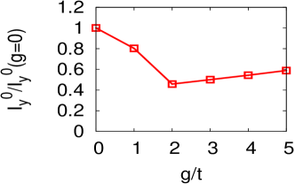
Figure 5: The surface current $I_{y}^{0}$ normalized by $I_{y}^{0}(g=0)$ in the absence of surface disorder, $V_{0}=0$.

The surface current is suppressed by the $p_{y}$-wave superfluidity. It is noted that similar behaviors are also seen for spatially uniform gap functions whose amplitudes are chosen to be consistent with the self consistent calculations. For non-self-consistent gap functions, we can tune the gap amplitudes $\Delta_{1,2}$ for each orbital independently in order to investigate $\Delta_{1,2}$-dependence of the surface current. By calculating the surface currents for such $\Delta_{1,2}$ we see that $I_{y}^{0}$ is determined by detailed balance between the gap amplitudes for the two orbitals (not shown). In the self consistent calculations, ratio between $\Delta_{1,2}$ is determined by the gap equation, which then leads to the non-monotonic behavior of $I_{y}^{0}(g)$ (Fig. 5).

In the presence of the surface perturbation potential $V_{ill^{\prime}}$, the current density is modified as in the previous section. We find that the resulting left surface current $I_{y}^{L}$ can also be changed from $I_{y}^{0}$ in contrast to U(1) symmetric systems, while $I_{y}^{R}$ is unchanged. For the random potential, the surface current $I_{y}^{L}$ is suppressed as shown in Fig. 6. $I_{y}^{L}$ is almost unchanged up tp $V_{0}\simeq t$, and it decreases by further increasing $V_{0}$. The reduction of $I_{y}^{L}$ by the surface roughness well agrees with our naive expectation that disorder would generally suppress surface currents. On the other hand, for the constant potential along the left surface sites, $(V_{i1},V_{i2},V_{i12})=(V_{0},0,0)$, the surface current $I_{y}^{L}$ shows non-monotonic $V_{0}$-dependence. $I_{y}^{L}$ is quickly suppressed as $V_{0}$ is introduced, and then it turns to increase exceeding $I_{y}^{0}$ when $V_{0}$ is sufficiently large. In order to understand this behavior, we show the current density $j_{yi}$ in Fig. 7. As $V_{0}$ is increased, $j_{yi}$ gets suppressed at the left surface sites $i=(x=0,y)$, but at the same time, it is increased at the next surface sites $i=(x=1,y)$. The reduction at $x=0$ sites determines $I_{y}^{L}$ for small $V_{0}\ll t$, while $I_{y}^{L}$ is dominated by the contribution from $x=1$ sites for large $V_{0}$. Since we now do not have U(1) symmetry and an associated sum rule, these changes in $j_{y}$ do not necessarily cancel out and indeed they add up to give non-trivial finite values. Therefore, $I_{y}^{L}$ deviates from $I_{y}^{0}$ and shows the non-monotonic behavior in the present system.

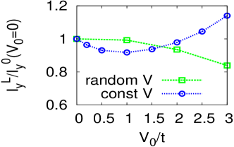
Figure 6: The surface current $I_{y}^{L}$ normalized by $I_{y}^{0}(V_{0}=0)$ when $g=5t$.

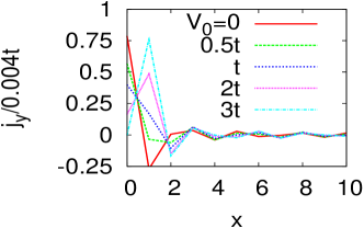
Figure 7: The current density $j_{y}$ near the left surface for the constant surface potential $(V_{i1},V_{i2})=(V_{0},0)$.

III.2.2 chiral $p$-wave superfluid

As a second example of superfluids without time reversal symmetry, we study a chiral $p$-wave superfluid on a square lattice in which surface current is generated by the superfluidity itself. The problem of spontaneous surface current and corresponding OAM, often referred to as “intrinsic angular momentum paradox”, has been discussed for more than 40 years  Leggett (1975); Vollhart and Wölfle (1990); Volovik (2003); Leggett (2006); Ishikawa et al. (1980); Mermin and Muzikar (1980); Kita (1998); Goryo (1998); Furusaki et al. (2001); Stone and Roy (2004); Mizushima et al. (2008); Sauls (2011); Bradlyn et al. (2012); Shitade and Kimura (2014); Hoyos et al. (2014); Tsutsumi (2014); Volovik (2015); Tada et al. (2015); Huang et al. (2014). Although most of the previous studies focus only on the weak coupling BCS region, here we discuss both the BCS region and the BEC region on an equal footing. In the present study, similarly to the previous models, surface roughness is introduced as a typical example of surface perturbations. We consider the following Hamiltonian

$$H_{p\rm SF} =\sum_{\rm NN}-t_{ij}c^{\dagger}_{i\sigma}c_{j\sigma}-g\sum_{{\rm NN}}n_{i\sigma}n_{j\bar{\sigma}}+H_{\rm surf},$$ (40)

$$H_{\rm surf} =\sum V_{i}n_{i\sigma},$$

where $V_{i}$ is finite only at the left surface, $i=(x=1,y)$. The hopping and interaction are allowed only for the nearest neighbor sites, and the same cylinder geometry as in the previous sections is used. The system size is $N_{x}\times N_{y}=60\times 20$, and we have confirmed finite size effects are negligibly small for this size by performing similar calculations for other sizes. We perform mean field calculations of the superfluidity, which is a good approximation even for a large $g$ at zero temperature since there are no thermal fluctuations in the ground states  Eagles (1969); Leggett (1980); Giorgini et al. (2008). The current density is simply

$$j_{\mu i} =\sum_{\sigma}-it[c^{\dagger}_{i\sigma}c_{i+\hat{\mu}\sigma}-c^{\dagger}_{i+\hat{\mu}\sigma}c_{i\sigma}].$$ (41)

Before discussing surface disorder effects, we first examine basic properties of the model in the absence of surface disorder. The present model exhibits a quantum phase transition  Read and Green (2000); Massignan et al. (2010) when $\mu=\mu_{c}=-4t$. For $|\mu|<|\mu_{c}|$, the system is in the BCS region where there are gapless chiral edge modes at the surfaces, while for $|\mu|>|\mu_{c}|$, the system is in the BEC region where there is a spectrum gap. In Fig. 8, we show the chemical potential $\mu$, amplitudes of the gap functions at a center site of the system $\Delta$, and spectrum gap $\delta E$ for fixed filling $n=0.2$.

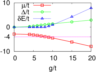
Figure 8: The chemical potential $\mu$, amplitude of the gap functions in the bulk $\Delta$, and spectrum gap $\delta E$ for filling $n=0.2$. The purple dotted line represent $\mu_{c}=-4t$.

The quantum phase transition takes place around $g\simeq 8t-9t$ for this filling where $\mu$ crosses $\mu_{c}$, and we have confirmed that similar behaviors are seen for other low filling. It is noted that, when filling is high, $n\simeq 1$, the ground state stays in the BCS region even for large $g$ and it is hard to realize the BCS-BEC phase transition.

We show the current density $j_{y}$ at $n=0.2$ for $g=5t$ (BCS region) and $g=15t$ (BEC region) in Fig. 9 as an example. $j_{x}$ vanishes everywhere in the system. The current density in the BEC region is more strongly localized near the surface than that in the BCS region, and it oscillates in sign depending on the distance from the surface. As a result, the surface current in the BEC region is smaller than that in the BCS region in the present lattice model, as shown in Fig. 10.

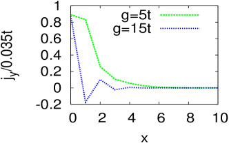
Figure 9: The current density $j_{y}$ near the left surface for $V_{0}=0$ at $n=0.2$ with $g=5t$ (BCS state, green) and $g=15t$ (BEC region, blue).

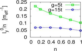
Figure 10: The surface current for different filling $n$ at $g=5t$ and $g=15t$ in unit of the effective mass $m_{\rm eff}=1/(2ta^{2})$.

We see that the overall behavior of $I_{y}^{0}$ in the BCS region as a function of filling $n$ is consistent with the recent work com (c). The surface current for low filling and weak coupling limit approaches $I=n/(4m_{\rm eff})$ where $m_{\rm eff}$ is an effective mass $m_{\rm eff}=1/(2ta^{2})$ with the lattice constant $a$. Under an assumption that the surface current is constant along a boundary of a finite system, this gives the OAM $L_{z}=m_{\rm eff}\oint[\mbox{\boldmath$r$}\times\mbox{\boldmath$I$}]_{z}dl=N/2$ where $N$ is the total number of fermions in agreement with the previous calculations for continuum systems without lattice potentials  Sauls (2011); Tsutsumi (2014); Volovik (2015); Tada et al. (2015). In the present lattice model, in contrast to the continuum systems where $L_{z}=N/2$ holds both in the weak coupling region and strong coupling region, $I_{y}$ and the corresponding OAM $L_{z}$ is decreased when the coupling constant $g$ is increased. This is because, even for low filling $n\ll 1$ where lattice effects is expected to be less important, the smallest size of a bosonic molecule of two fermions is bounded by the lattice constant for a non-$s$-wave superfluid on a lattice, and therefore, presence of a lattice is significant especially for the BEC region rather than the BCS region. Because of this lattice effect, the surface current per fermion for strong $g=15t$ is almost independent of filling as seen in Fig. 10, although the system stays in the BCS region for high filling $n\simeq 1$.

Now, we discuss effects of the surface disorder. The current density $j_{y}$ averaged over disorder configurations for $n=0.2$ at a large $V_{0}=8t$ is shown in Fig. 11.

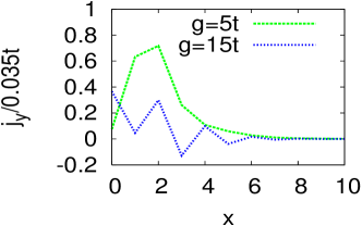
Figure 11: The current density $j_{y}$ near the left surface for $V_{0}=8t$ at $n=0.2$ with $g=5t$ (BCS state, green) and $g=15t$ (BEC region, blue).

For the BCS region, $j_{y}$ is suppressed especially at the surface sites $x=0$ and it is enhanced at inner sites $x=3,4$ to partly compensate the reduction, while $j_{y}$ in the BEC region becomes strongly oscillating and effects of $V_{i}$ propagate into further inner sites $x=4,5$. As in the previous model (III.2.1), change of $j_{y}$ does not need to obey a sum rule and the surface current can be modified from $I_{y}^{0}$.

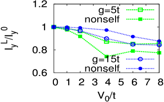
Figure 12: The left surface current $I_{y}^{L}$ for different $V_{0}$ at $g=5t$ (green square) and $g=15t$ (blue circle) when filling is $n=0.2$. Filled symbols correspond to non-self-consistent gap functions whose amplitudes are chosen to be consistent with self consistent calculations at $g=5t$ and $g=15t$, respectively.

Indeed, as shown in Fig. 12, the surface current is suppressed by the surface disorder. The decrease of $I_{y}^{L}$ in the weak coupling BCS limit is consistent with the previous studies Sauls (2011); Ashby and Kallin (2009); Nagato et al. (2011). Interestingly, $I_{y}^{L}$ decreases not only in the BCS region but also in the BEC region. This would be because the smallest bosonic molecule size is bounded by the lattice constant and the disorder length scale is of the same order in the present model. We have confirmed similar behaviors of $I_{y}^{L}$ for different parameter sets $(g,n)$. For a comparison, we also calculate surface currents for non-self-consistent gap functions which are constant in space and whose amplitudes are chosen to be consistent with the self-consistent calculations. The surface currents are suppressed in a similar way as in the self consistent calculations, which means that change of the gap functions around the surface by $H_{\rm surf}$ is not important for the reduction of $I_{y}$. We note that, although the reduction of $I_{y}^{L}$ by the surface disorder is moderate, it was pointed out that, for domain boundaries with opposite chiralities in the BCS region, the boundary current strongly relies on boundary conditions and it can change even its direction Tsutsumi (2014); Volovik (2015).

III.3 discussion

We have discussed suppression of surface currents in cylinder systems in the previous sections. For a realistic finite size system with open boundary conditions for all directions, surface current flows along the surface and generates global rotation. In the absence of surface perturbations, its magnitude is obviously uniform along the surface. If some parts of the surface are perturbed, the surface current would be changed not only at the perturbed surface but also at the whole surface, because of the continuity of the current density. Therefore, associated OAM would also be modified.

Although we have examined particular realizations of surface potentials among possible surface perturbations, existence of surface perturbations which change $I_{y}$ conceptually distinguishes a system without U(1) symmetry from a system with U(1) symmetry. The surface current is not uniquely determined as a bulk property and there may exist surface perturbations which drastically change it in the former, while the surface current is an intrinsic quantity in the latter. The absence of a sum rule for the surface current density and the numerical results suggest that there is no bulk-surface correspondence for surface currents and corresponding OAM in superfluids, and surface conditions should be fully taken into account in order to calculate these quantities in contrast to some of the previous studies for chiral superfluids  Bradlyn et al. (2012); Shitade and Kimura (2014). From these discussions, it is considered that surface currents and OAM in superfluids with broken time reversal symmetry would be subtle quantities, and experimentally, one needs to control surface conditions carefully in order to measure these quantities.

Let us briefly discuss the change of surface currents and OAM in superfluids in view of thermodynamics. In the present study, we have implicitly assumed that the lattices (or containers for non-lattice systems) are at rest in the laboratory frame by some reasons. If the lattice or container is fixed spatially to a much larger environment, the system composed only of the superfluid and lattice does not conserve the OAM and it is an open system with respect to angular momentum. Although OAM of the superfluid alone can be changed by surface perturbations, total OAM of the whole system including the large environment should be a conserved thermodynamic quantity and is independent of surface details of the lattice/container. If the system composed of a superfliud and a lattice/container is suspended in the midair and set to be at rest, as temperature is decreased down to the superfluid transition temperature, the lattice/container should start to rotate in an opposite direction to the superfluid rotation in order to keep the total OAM of the whole system zero due to the angular momentum conservation. This is analogous to the Einstein-de Haas effect and each of the OAM for the superfluid and lattice/container would depend on surface conditions in the present system.

In the present study, we have not taken into account the electromagnetic field which couples to charged particles. Indeed, it is especially important in superconductors which exhibit Meissner effect. If Meissner effect is included, current density distributions are modified and net surface currents would vanish for uniform superconducting states Furusaki et al. (2001); Ashby and Kallin (2009). The problem of Meissner effect would be more complicated in a system where there exist circulating currents even in non-superconducting states, such as the model (III.2.1) and ferromagnetic superconductors. This issue is left for a future work.

When we were finalizing the present paper, we became aware of a relevant article by  Kusama and Ohashi (1999) which claims that, when surface currents are not canceled between left and right surfaces in a cylinder, supercurrent will compensate this and total current will vanish in superfluids. Although this is an important possibility for a vanishing total current, this issue has not been well understood. For example, in Kusama and Ohashi (1999), the current density even near the non-perturbed surface is strongly changed from the original configuration if supercurrent is included. This seems unphysical, since effects of local perturbations only on a surface should not propagate to the opposite surface. Secondly, although they compared the free energy density of different system sizes for a technical reason, this cannot be justified in general. Their discussion is motivated by the original Bloch-Bohm’s theorem which is not helpful for surface currents as shown in Sec. II.2, and further investigations would be required to understand this issue. Here, in order to have an insight, let us breify consider a possible supercurrent in a cylinder $L\times L$ where open (periodic) boundary condition is imposed for $x(y)$-direction, and surface perturbations are introduced only for one surface. Supercurrent density is roughly proportional to $\nabla\phi(x,y)$ for a gap function $\Delta=e^{i\phi}\tilde{\Delta}$ where $\tilde{\Delta}$ is a gap function without a modulation. In the cylinder considered, the supercurrent density $\sim\nabla\phi$ should be translationally symmetric along the $y$-direction. Therefore, $\phi$ must be $\phi=q_{x}x+q_{y}y$ with $q_{\mu}=2\pi n/L,(n=0,\pm 1,\cdots)$, and $q_{x}$ should be zero for a vanishing total supercurrent in the $x$-direction. Besides, $q_{y}$ should be of order $2\pi/L$ so that the current density near the non-perturbed surface remains unchanged. In such a case, $q_{y}\simeq 2\pi/L$ introduces supercurrent density $\sim 1/L$ at every site, resulting in a total supercurrent $\sim L$ ($L^{d-1}$ in $d$-dimensions) in the whole system, which is the same order as the surface current. We note that, however, two thermodynamic states constructed from wavefunctions with $\Delta$ and $\tilde{\Delta}$ respectively could not be distinguished by local operators and therefore they converge to a single state as in Sec. II.2. Besides, if we consider a semi-infinite system and discuss it within weak coupling approximations as in the previous studies Ashby and Kallin (2009); Nagato et al. (2011), we could not impose a boundary condition at infinite with an infinitesimal supercurrent density. Furthermore, if we consider a realistic finite size sample with boundaries and introduce surface roughness, it is impossible to realize a uniform supercurrent density and possible current density configuration especially near the surface would be quite complicated. Therefore, possible compensation by supercurrent is a subtle issue. In order to discuss such a subtle issue, we would also have to be careful about validity of the mean field approximations. Further investigations of gap functions and supercurrent may be required for clarifying a role of supercurrents.

IV summary

In summary, we have investigated equilibrium surface currents in systems with or without U(1) particle number conservation. For the systems with U(1) symmetry, we showed that the surface currents are independent of surface perturbations based on the sum rule for current densities, which was confirmed by numerical calculations for a concrete model with surface perturbations. Therefore, the surface currents and corresponding orbital magnetization are bulk quantities which are robust against surface conditions. The sum rule argument is also applicable to the Landau diamagnetism, and it would give a new understanding on the known equivalence between the bulk approaches and the surface approaches. On the other hand, in superfluids which do not have U(1) symmetry, the surface currents are changed by surface perturbations. Especially, in a chiral superfluid on a lattice, the surface current is suppressed by surface disorder not only in the weak coupling BCS region but also in the strong coupling BEC region. These results imply that surface mass currents and orbital angular momentum in superfluids with broken time reversal symmetry would be subtle quantities and depend on surface details. Experimentally, one needs to control surface conditions carefully in order to measure these quantities.

Appendix A. Sum Rule for Continuum Model

Our sum rule argument holds also for continuum models with lattice potentials. We consider a general Hamiltonian defined on a cylinder $L\times L$ with the open (periodic) boundary condition for $x(y)$-direction,

$$H =\int_{L^{2}}d^{2}x\psi^{\dagger}{\mathcal{K}}\psi+H_{\rm int}+H_{\rm surf},$$ (A1)

where ${\mathcal{K}}$ is the single-particle Hamiltonian including the lattice potential and $\psi(\mbox{\boldmath$r$})=(\psi_{\uparrow}(\mbox{\boldmath$r$}),\psi_{\downarrow}(\mbox{\boldmath$r$}))$ is the fermionic field operator. Then we expand the field operator in terms of non-interacting single-particle wavefunctions,

$$\psi(\mbox{\boldmath$r$})=\sum_{k_{y}n}\varphi_{k_{y}n}(\mbox{\boldmath$r$})c_{k_{y}n},$$ (A2)

$${\mathcal{K}}\varphi_{k_{y}n}=\varepsilon_{k_{y}n}\varphi_{k_{y}n},$$ (A3)

where $k_{y}$ is Bloch wavenumber along the $y$-direction and $n$ represents other indices including a quantum number corresponding to position $x$. The Matsubara Green’s function $G(r,r^{\prime})=-\langle\langle\psi(r)\psi^{\dagger}(r^{\prime})\rangle\rangle$ is also expanded as

$$G(\mbox{\boldmath$r$},\mbox{\boldmath$r$}^{\prime},i\omega) =\sum_{k_{y}nn^{\prime}}\varphi_{k_{y}n}(\mbox{\boldmath$r$})g_{nn^{\prime}}(k_{y},i\omega)\varphi_{k_{y}n^{\prime}}^{\ast}(\mbox{\boldmath$r$}^{\prime}),$$ (A4)

$$\hat{g}(k_{y},i\omega,) =[\hat{g}_{0}^{-1}-\hat{\Sigma}]^{-1},$$ (A5)

where $(g_{0})^{-1}_{nn^{\prime}}=[i\omega-\varepsilon_{k_{y}n}]\delta_{nn^{\prime}}$ is the non-interacting Green’s function and $\hat{\Sigma}$ is the selfenergy in the $\varphi_{k_{y}n}$-basis. Similarly to the lattice models, spontaneous symmetry breaking order parameters are easily incorporated into $g$. In the cylinder, the surface current averaged over the $y$-direction is simply given by

$$I_{y}^{L(R)} =\frac{1}{L}\int_{S_{L}(S_{R})}d^{2}xj_{y}(\mbox{\boldmath$r$})$$

$$=\frac{1}{L}\sum_{i\in S_{L}(S_{R})}\int_{v_{i}}d^{2}xj_{y}(\mbox{\boldmath$r$}),$$ (A6)

where $j_{y}$ is the current density. As discussed in the main text and Ref. com, a, contributions to the surface current come only from $S_{L}(S_{R})$ and not from bulk regions. Therefore, when U(1) charge symmetry is present, the total surface current $I_{y}^{\rm tot}=\langle I_{y}^{L}+I_{y}^{R}\rangle$ is written as

$$I_{y}^{\rm tot} =\frac{1}{L}\int_{L^{2}}d^{2}x\langle j_{y}(\mbox{\boldmath$r$})\rangle$$

$$=\frac{1}{L}\int_{L^{2}}d^{2}x\frac{-i}{2m}[\partial_{y^{\prime}}-\partial_{y}]G(\mbox{\boldmath$r$},\mbox{\boldmath$r$}^{\prime},\tau=0^{-})|_{r=r^{\prime}}$$

$$=-\frac{1}{L}\sum_{k_{y}}{\rm tr}\Bigl{[}\frac{\partial\hat{g}_{0}^{-1}(k)}{\partial k_{y}}\hat{g}(k)\Bigr{]}.$$ (A7)

Here, trace describes summation over $n$ and $\omega$. We can now follow the same argument as in the main text, and show $I^{\rm tot}_{y}=0$ even in the presence of left surface perturbations. This means that the surface current is unchanged by surface perturbations.

It is noted that the surface currents in lattice models are obtained by the following replacement in Eq. (A6),

$$\sum_{i\in{\rm surf}}\int_{v_{i}}d^{2}x\psi^{\dagger}(-i\partial_{y})\psi$$

$$=\sum_{i\in{\rm surf}}\sum_{RR^{\prime},ll^{\prime}}\langle w_{Rl}|-i\partial_{y}|w_{R^{\prime}l^{\prime}}\rangle_{v_{i}}c^{\dagger}_{Rl}c_{R^{\prime}l^{\prime}}$$

$$\rightarrow\sum_{RR^{\prime}\in{\rm surf}}\sum_{ll^{\prime}}\langle w_{Rl}|-i\partial_{y}|w_{R^{\prime}l^{\prime}}\rangle c^{\dagger}_{Rl}c_{R^{\prime}l^{\prime}},$$ (A8)

where $w_{Rl}$ is a Wannier function and $\langle\cdots\rangle_{v_{i}}=\int_{v_{i}}d^{2}x$. This replacement is verified when the chosen Wannier function is well localized in a length scale which is much smaller than the system size. By similar replacements, other local site quantities such as particle density at site $i$ become equivalent to the usual Wannier basis descriptions, $\int_{v_{i}}d^{2}x\psi^{\dagger}\psi=\sum_{RR^{\prime}ll^{\prime}}\langle w_{Rl}|w_{R^{\prime}l^{\prime}}\rangle_{v_{i}}c^{\dagger}_{Rl}c_{R^{\prime}l^{\prime}}\rightarrow\sum_{R=R^{\prime}\in v_{i}}\sum_{ll^{\prime}}\langle w_{Rl}|w_{R^{\prime}l^{\prime}}\rangle c^{\dagger}_{Rl}c_{R^{\prime}l^{\prime}}=\sum_{l}c^{\dagger}_{R_{i}l}c_{R_{i}l}$. Even when the replacement of the surface current operator is legitimate, however, the resulting surface current might depend on Wannier functions or gauge of Bloch functions Thonhauser et al. (2005); Ceresoli et al. (2006), although the original definition (A6) is independent of them.

References

- Martin (2004) R. M. Martin, Electronic Structure: Basic Theory and Practical Methods (Cambridge University Press, 2004), 1st ed.
- Hasan and Kane (2010) M. Z. Hasan and C. L. Kane, Rev. Mod. Phys. 82, 3045 (2010).
- Qi and Zhang (2011) X. L. Qi and S. C. Zhang, Rev. Mod. Phys. 83, 1057 (2011).
- Wen (2004) X. G. Wen, Quantum Field Theory of Many-Body Systems (Oxford University Press, 2004), 1st ed.
- Gat and Avron (2003a) O. Gat and J. E. Avron, Phys. Rev. Lett. 91, 186801 (2003a).
- Gat and Avron (2003b) O. Gat and J. E. Avron, New J. Phys. 5, 44 (2003b).
- Xiao et al. (2005) D. Xiao, J. Shi, and Q. Niu, Phys. Rev. Lett. 95, 137204 (2005).
- Thonhauser et al. (2005) T. Thonhauser, D. Ceresoli, D. Vanderbilt, and R. Resta, Phys. Rev. Lett. 95, 137205 (2005).
- Ceresoli et al. (2006) D. Ceresoli, T. Thonhauser, D. Vanderbilt, and R. Resta, Phys. Rev. B 74, 024408 (2006).
- Shi et al. (2007) J. Shi, G. Vignale, D. Xiao, and Q. Niu, Phys. Rev. Lett. 99, 197202 (2007).
- Resta (2010) R. Resta, J. Phys.:Condens. Matter 22, 123201 (2010).
- Thonhauser (2011) T. Thonhauser, Int. J. Mod. Phys. B 25, 1429 (2011).
- Xiao et al. (2010) D. Xiao, M. C. Chang, and Q. Niu, Rev. Mod. Phys. 82, 1959 (2010).
- Matsumoto and Murakami (2011) R. Matsumoto and S. Murakami, Phys. Rev. Lett. 106, 197202 (2011).
- Chen and Lee (2011) K. T. Chen and P. A. Lee, Phys. Rev. B 84, 205137 (2011).
- Chen and Lee (2012) K. T. Chen and P. A. Lee, Phys. Rev. B 86, 195111 (2012).
- Leggett (1975) A. J. Leggett, Rev. Mod. Phys. 47, 331 (1975).
- Vollhart and Wölfle (1990) D. Vollhart and P. Wölfle, The Superfluid Phase of Helium 3 (Taylor and Francis, London, 1990), 1st ed.
- Volovik (2003) G. E. Volovik, The Universe in a Helium Droplet (Oxford University Press, Oxford, 2003).
- Leggett (2006) A. J. Leggett, Quantum Liquids: Bose Condensation and Cooper Pairing in Condensed-matter Systems (Oxford University Press, Oxford, 2006).
- Ishikawa et al. (1980) M. Ishikawa, K. Miyake, and T. Usui, Prog. Theor. Phys. 63, 1083 (1980).
- Mermin and Muzikar (1980) N. D. Mermin and P. Muzikar, Phys. Rev. B 21, 980 (1980).
- Kita (1998) T. Kita, J. Phys. Soc. Jpn. 67, 216 (1998).
- Goryo (1998) J. Goryo, Phys. Lett. A 246, 549 (1998).
- Furusaki et al. (2001) A. Furusaki, M. Matsumoto, and M. Sigrist, Phys. Rev. B 64, 054514 (2001).
- Stone and Roy (2004) M. Stone and R. Roy, Phys. Rev. B 69, 184511 (2004).
- Mizushima et al. (2008) T. Mizushima, M. Ichioka, and K. Machida, Phys. Rev. Lett. 101, 150409 (2008).
- Sauls (2011) J. A. Sauls, Phys. Rev. B 84, 214509 (2011).
- Bradlyn et al. (2012) B. Bradlyn, M. Goldstein, and N. Read, Phys. Rev. B 86, 245309 (2012).
- Shitade and Kimura (2014) A. Shitade and T. Kimura, Phys. Rev. B 90, 134510 (2014).
- Hoyos et al. (2014) C. Hoyos, S. Moroz, and D. T. Son, Phys. Rev. B 89, 174507 (2014).
- Tsutsumi (2014) Y. Tsutsumi, J. Low Temp. Phys. 175, 51 (2014).
- Volovik (2015) G. E. Volovik, JETP Letters 100, 742 (2015).
- Tada et al. (2015) Y. Tada, W. Nie, and M. Oshikawa, Phys. Rev. Lett. 114, 195301 (2015).
- Huang et al. (2014) W. Huang, E. Taylor, and C. Kallin, Phys. Rev. B 90, 224519 (2014).
- Mackenzie and Maeno (2003) A. P. Mackenzie and Y. Maeno, Rev. Mod. Phys. 75, 657 (2003).
- Maeno et al. (2012) Y. Maeno, S. Kittaka, T. Nomura, S. Yonezawa, and K. Ishida, J. Phys. Soc. Jpn. 81, 011009 (2012).
- Ashby and Kallin (2009) P. E. C. Ashby and C. Kallin, Phys. Rev. B 79, 224509 (2009).
- Nagato et al. (2011) Y. Nagato, S. Higashitani, and K. Nagai, J. Phys. Soc. Jpn. 80, 113706 (2011).
- Read and Green (2000) N. Read and D. Green, Phys. Rev. B 61, 10267 (2000).
- Luttinger (1960) J. M. Luttinger, Phys. Rev. 119, 1153 (1960).
- Luttinger and Ward (1960) J. M. Luttinger and J. C. Ward, Phys. Rev. 118, 1417 (1960).
- Yamanaka et al. (1997) M. Yamanaka, M. Oshikawa, and I. Affleck, Phys. Rev. Lett. 79, 1110 (1997).
- Oshikawa (2000) M. Oshikawa, Phys. Rev. Lett. 84, 3370 (2000).
- Dzyaloshinskii (2003) I. Dzyaloshinskii, Phys. Rev. B 68, 085113 (2003).
- com (a) If contributions to surface currents from current density were not localized around a surface, corresponding OM/OAM would not be proportional to area of a system since where is typical system length and . Even if magnitude of is not exponentially decreasing and is oscillating away from a surface in a gapless system, contributions to surface currents from bulk regions would be negligible, because effects of a surface should be vanishingly small in the bulk regions and the bulk regions preserves the same translational symmetry as in the periodic boundary condition case. Besides, a surface region can be well identified when there is nearly uniform current density in the bulk which varies in a length scale much smaller than the system size. In this case, we can define the surface region so that the current density becomes nearly uniform (in the above sense) outside of it. Therefore, in general systems, there exists an appropriate surface region whose width is much smaller than the system size and surface currents are well defined by .
- com (b) We note that the Luttinger-Ward indentity holds in the presence of both interactions and surface perturbations. For disorder surface perturbations, we sum up all the closed skeleton diagrams in terms of the averaged Green’s function and construct a “Luttinger-Ward functional” as in clean systems, whose derivative with respect to gives the averaged selfenergy. Then, we consider with , which is a sum of all the closed skeleton diagrams but one -line is replaced by -line for every diagram. Following the original argument for the Luttinger-Ward identity Luttinger (1960); Luttinger and Ward (1960), it is now easily seen that holds due to the -momentum conservation. By performing a partial integral, we obtain the Luttinger-Ward identity.
- Rosch (2007) A. Rosch, Eur. Phys. J. B 59, 495 (2007).
- Dave et al. (2013) K. B. Dave, P. W. Phillips, and C. L. Kane, Phys. Rev. Lett. 110, 090403 (2013).
- Landau (1930) L. D. Landau, Z. Phys. 64, 629 (1930).
- Peierls (1933) R. Peierls, Z. Phys. 80, 763 (1933).
- Fukuyama (1971) H. Fukuyama, Prog. Theor. Phys. 45, 704 (1971).
- Kubo (1964) R. Kubo, J. Phys. Soc. Jpn. 19, 2127 (1964).
- Ohtaka and Moriya (1973) K. Ohtaka and T. Moriya, J. Phys. Soc. Jpn. 34, 1203 (1973).
- Ishikawa and Fukuyama (1999) Y. Ishikawa and H. Fukuyama, J. Phys. Soc. Jpn. 68, 2405 (1999).
- Nee et al. (1968) T. W. Nee, J. F. Koch, and R. E. Prange, Phys. Rev. 174, 758 (1968).
- Abrikosov (1988) A. A. Abrikosov, Fundamentals of the Theory of Metals (North Holland, 1988).
- Bohm (1949) D. Bohm, Phys. Rev. 75, 502 (1949).
- Vignale (1995) G. Vignale, Phys. Rev. B 51, 2612 (1995).
- Ohashi and Momoi (1996) Y. Ohashi and T. Momoi, J. Phys. Soc. Jpn. 65, 3254 (1996).
- Kusama and Ohashi (1999) Y. Kusama and Y. Ohashi, J. Phys. Soc. Jpn. 68, 987 (1999).
- Lieb et al. (1961) E. Lieb, T. Schultz, and D. Mattis, Ann. Phys. 16, 407 (1961).
- Carruthers and Nieto (1968) P. Carruthers and M. M. Nieto, Rev. Mod. Phys. 40, 411 (1968).
- Emch (1972) G. G. Emch, in Phase Transitions and Critical Phenomena (Academic Press, London, 1972), vol. 1, chap. 4.
- Eschrig et al. (1985) H. Eschrig, G. Seifert, and P. Ziesche, Solid State Commun. 56, 777 (1985).
- Vignale and Rasolt (1987) G. Vignale and M. Rasolt, Phys. Rev. Lett. 59, 2360 (1987).
- Higuchi and Hasegawa (1997) M. Higuchi and A. Hasegawa, J. Phys. Soc. Jpn. 66, 149 (1997).
- Streda (1982) P. Streda, J. Phys. C 15, L717 (1982).
- MacDonald (1995) A. H. MacDonald, in Mesoscopic Quantum Physics (Les Houches, Session LXI) (North Holland, Amsterdam, 1995).
- Kaur et al. (2005) R. P. Kaur, D. F. Agterberg, and M. Sigrist, Phys. Rev. Lett. 94, 137002 (2005).
- Yip (2005) S. K. Yip, J. Low Temp. Phys. 140, 67 (2005).
- Eagles (1969) D. M. Eagles, Phys. Rev. 186, 456 (1969).
- Leggett (1980) A. J. Leggett, in Modern Trends in the Theory of Condensed Matter, edited by A. Pekalski and J. Przystawa (Springer, Berlin, 1980).
- Giorgini et al. (2008) S. Giorgini, L. P. Pitaevskii, and S. Stringari, Rev. Mod. Phys. 80, 1215 (2008).
- Massignan et al. (2010) P. Massignan, A. Sanpera, and M. Lewenstein, Phys. Rev. A 81, 031607(R) (2010).
- com (c) A. Tsuruta and K. Miyake, unpublished.