No galaxy left behind: accurate measurements with the faintest objects in the Dark Energy Survey

Abstract

Accurate statistical measurement with large imaging surveys has traditionally required throwing away a sizable fraction of the data. This is because most measurements have relied on selecting nearly complete samples, where variations in the composition of the galaxy population with seeing, depth, or other survey characteristics are small.

We introduce a new measurement method that aims to minimize this wastage, allowing precision measurement for any class of detectable stars or galaxies. We have implemented our proposal in Balrog, software which embeds fake objects in real imaging to accurately characterize measurement biases.

We demonstrate this technique with an angular clustering measurement using Dark Energy Survey (DES) data. We first show that recovery of our injected galaxies depends on a variety of survey characteristics in the same way as the real data. We then construct a flux-limited sample of the faintest galaxies in DES, chosen specifically for their sensitivity to depth and seeing variations. Using the synthetic galaxies as randoms in the Landy-Szalay estimator suppresses the effects of variable survey selection by at least two orders of magnitude. With this correction, our measured angular clustering is found to be in excellent agreement with that of a matched sample from much deeper, higher-resolution space-based Cosmological Evolution Survey (COSMOS) imaging; over angular scales of $0.004\degr<\theta<0.2\degr$, we find a best-fit scaling amplitude between the DES and COSMOS measurements of $1.00\pm 0.09$.

We expect this methodology to be broadly useful for extending measurements’ statistical reach in a variety of upcoming imaging surveys.

1 Introduction

Wide-field optical surveys have played a central role in modern astronomy. The Sloan Digital Sky Survey (SDSS, York et al., 2000) alone has furnished nearly 6,000 publications across a wide variety of subjects: from star formation, to galaxy evolution, to measuring cosmological parameters; among a multitude of others. The discovery of cosmic acceleration (Riess et al., 1998, Perlmutter et al., 1999) has motivated several expansive imaging surveys for the future: for instance, the Large Synoptic Survey Telescope, the Wide-Field Infrared Survey Telescope (Dressler et al., 2012), and Euclid (Laureijs et al., 2012). The legacy of these next-generation imaging efforts will almost certainly yield an even richer harvest than what has come before them.

With large surveys, astronomical sample sizes have grown, increasing the statistical power of their measurements; with great power comes great responsibility (see e.g. Lee et al., 1962) for control of systematic errors. Taking full advantage of these data means ensuring that the precision of these measurements is matched by their accuracy. At present time, however, high-precision measurements are generally made with samples drawn from only the fraction of the data that is nearly complete. We argue that the current state of the art in survey astronomy is in many ways wasteful of information, and lay out a general method for improvement.

This paper focuses on measurements of the galaxy angular correlation function for highly incomplete, flux-limited samples of galaxies, especially near the detection threshold. We have chosen this approach for two reasons. First, this measurement is an especially challenging example of systematic error mitigation; we show below that, for our faintest galaxies, we will have to eliminate systematic biases that are much larger than our signal, and do so over a wide range of survey conditions. The second reason is that systematic effects relevant for angular clustering measurements also directly impact probes of cosmic acceleration (Weinberg et al., 2013), where the requirements on systematic error control are particularly strict.

1.1 The current state of the art

Astronomers have been measuring galaxy clustering for several decades, since at least Zwicky (1937). The angular two-point correlation function, $w(\theta)$, is a common tool used to characterize the anisotropies in the galaxy ensemble. From the very beginning, efforts to measure $w(\theta)$ have been challenged by the presence of anisotropies in the data arising from imperfect measurements, or from astrophysical complications unrelated to large-scale structure.

A complete list of sources of systematic effects is difficult (if not impossible) to compile, but some issues are common to all extragalactic measurements, like star-galaxy separation and photometric calibration. Because the point spread function (PSF) varies across the survey area, the accuracy with which galaxies can be distinguished from stars will vary, introducing anisotropies associated with stellar contamination. Accurate, uniform photometric calibration for a multi-epoch wide-field optical survey is difficult to accomplish (Schlafly et al., 2012), and given the variations in seeing, airmass, transparency, and other observing conditions, uniform depth is generally unachievable. A wide variety of schemes have been used to ameliorate these complicating effects.

For a $w(\theta)$ measurement with the Automated Plate Measurement survey – among the earliest digitized sky surveys – Maddox et al. (1996) built models of the selection function, including plate measurement effects (e.g., the variation of the photographic emulsion’s sensitivity across each plate), observational effects (atmospheric extinction) and astrophysical effects (Galactic extinction). For each of these, they estimated the contribution of the systematic effect to the final $w(\theta)$ measurement. Stellar contamination was dealt with by subtracting estimated stellar densities from the map of galaxy counts in cells, and adjusting the amplitude of the final $w(\theta)$ measurement to compensate for the estimated dilution due to stellar contamination.

Similar measurements of $w(\theta)$ were made for validation purposes in the early SDSS data (Scranton et al., 2002). The authors here cross-correlated the measured galaxy densities with a number of known sources of systematic errors in order to determine which regions of the survey to mask.

Many subsequent SDSS analyses were based on a volume-limited sample of luminous red galaxies, from which $\sim\!120,000$ objects were targeted for SDSS spectroscopy (Eisenstein et al., 2001). Here again (see also Padmanabhan et al. 2007 for the properties of the parent photometric sample) the strategy was to use cross-correlation techniques to remove data that would imperil the analysis, leaving an essentially complete sample.

The targets selected for the larger SDSS-III Baryon Oscillation Spectroscopic Survey (BOSS) measurements (Schlegel et al., 2009) were substantially fainter, and the systematic error corrections for these samples necessarily more sophisticated. Ross et al. (2011b) explored several mitigation strategies for SDSS data. A linear model for the dependence of the galaxy counts as a function of potential sources of systematic errors was built, allowing for subtraction of the systematic effects from the final galaxy $w(\theta)$ measurement. For the most important systematic effects (constrained again by cross-correlation with the galaxies), galaxies in the $w(\theta)$ estimator were upweighted by the inverse of their detection probability. The BOSS baryon acoustic oscillation scale measurement in Ross et al. (2012) made use of this weighting scheme. With the exception of stellar occultation, these effects were mostly perturbative, and the errors on the angular clustering were large enough that the stellar occultation corrections only had to be characterized at the $\sim\!10\%$ level.

The imaging systematic error mitigation used by the WiggleZ spectroscopic survey (Blake et al., 2010) came closest to the spirit of this paper. Their spectroscopic target catalog was built by a combination of SDSS and Galaxy Evolution Explorer (GALEX) measurements. The blue emission-line galaxies targeted by WiggleZ were faint enough to be substantially affected by variations in the SDSS completeness, so the GALEX catalogs were used to estimate the variation of the target selection probability with various survey properties. Models were fit to this dependence, and the results were directly incorporated into the window function used in power spectrum estimation. The resulting corrections had a $\sim\!0.5\sigma$ effect on the final power spectrum, and so like SDSS only needed to be accurate at the $\sim\!10\%$ level.

This list is not exhaustive, but we believe it gives a fair picture of the state of the art. Generally, for their extragalactic clustering measurements, modern photometric surveys have relied on selecting a relatively complete sample, and then applying small corrections late in the analysis. We believe that this approach is a poor fit to the age of precision cosmology with ‘big data.’ The rest of this paper will present our proposed alternative.

1.2 Modeling the Dark Energy Survey selection function

We propose to measure the selection function of imaging surveys by embedding a realistic ensemble of fake star and galaxy images in the real survey data. The resulting measurement catalogs comprise a Monte Carlo sampling of the selection function and measurement biases of the survey, and can naturally account for systematic effects arising from the photometric pipeline, detector defects, seeing, and other sources of observational systematic errors. Several of the major systematic errors examined in the above measurements can be straightforwardly estimated and removed using the embedded catalogs, though astrophysical effects like dust and photometric calibration must of course be modeled using external data.

We test this technique using Dark Energy Survey (DES) imaging. DES is a $5-$year optical and near-infrared survey of $5,000~{}\mathrm{deg}^{2}$ of the South Galactic Cap, to $i_{AB}\leq 24$ (Dark Energy Survey Collaboration, 2005). The survey instrument, the Dark Energy Camera (DECam, Flaugher et al., 2015), was commissioned in fall 2012. During the Science Verification (SV) phase, which lasted from November 2012 to February 2013, data were taken over $\sim\!250~{}{\rm deg}^{2}$ in a manner mimicking the full 5-year survey, but with substantial depth variations (see e.g. Leistedt et al. 2015), mainly due to weather and early DECam operational challenges. Coadd images in each of the five bands, as well as a detection image combining the $riz$ filters, were produced from the $\sim\!10$ single-epoch exposures per filter.

Our work is complementary to that of Chang et al. (2015), who used generative modeling, in combination with outputs from the Blind Cosmology Challenge (Busha et al., 2013) and the Ultra Fast Image Generator (Bergé et al., 2013), to simulate DES-like data which were then run through the DES analysis pipeline (Mohr et al., 2012, Desai et al., 2012). A fully generative approach does have some advantages over the Monte Carlo sampling of the images described here. With a generative model, one can explore counterfactual realizations of the survey. This helps, for instance, in mapping out the interaction between the survey selection function and the galaxy population (for instance, how the angular clustering of galaxies interacts with the deblending and sky-subtraction algorithms). By construction, our embedding strategy considers only the single DES-realization of the survey properties.

However, the generative modeling approach is more sensitive to model mis-specification errors; it requires models not only for the noise, photometric calibration, star and galaxy ensemble properties, etc., but also for cosmic rays, bright stellar diffraction spikes, CCD defects, satellite trails, and other non-physical signatures that are difficult to model accurately. The embedded simulations, by contrast, inherit many of the properties of the image that are otherwise difficult to model. To keep the embedded population as realistic as possible, we draw our simulated stars and galaxies from catalogs made from high-resolution Hubble Space Telescope imaging.

1.3 Angular clustering in the Dark Energy Survey

Crocce et al. (2015) present a DES benchmark measurement of $w(\theta)$, adopting a standard approach to their clustering analysis by choosing a relatively complete sample ($i<22.5$) and masking potential sources of systematic errors traced by maps of the DES observing properties measured by Leistedt et al. (2015). In this paper, we use our Monte Carlo simulation framework to correct for the spatially-dependent completeness inhomogeneities, and then measure clustering signals at magnitudes well below the nominal limiting depth of $i<22.5$ used by Crocce et al. (2015).

The paper is organized as follows. In Section 2, we present Balrog, our software pipeline for embedding simulations into astronomical images. In Section 3, we describe our empirical procedure for generating a realistic ensemble of simulated sources, then prototype Balrog by injecting $\sim\!40,000,000$ simulated objects into $178~{}\mathrm{deg}^{2}$ of DES SV coadd images. We generate a synthetic catalog using the same procedure as is used for generation of the DES science catalogs. Section 4 validates that the photometric properties of the synthetic catalogs are a close match to those of the real DES catalogs for a wide range of quantities. If these synthetic catalogs really capture the variation in the survey selection function and measurement biases, it should be possible to use them as randoms to measure $w(\theta)$ accurately even for the faintest galaxies in the survey. We do exactly this in Section 5, demonstrating that our clustering measurements for the faintest DES galaxies ($23<i<24$) show excellent agreement with higher resolution external space-based data, which are complete over the selection range. The shapes of our $w(\theta)$ curves match general expectation. Section 6 concludes with a discussion of our results.

2 Balrog Implementation

Figure 1: High-level overview of Balrog’s processing. Shape usage follows standard flowchart notation. White parallelograms are inputs, dark gray parallelograms are outputs, and light gray rectangles are processes/commands. (The simulation truth catalog is coupled with the measurement software because by default Balrog runs SExtractor in association mode, using the simulation positions as the matching list, cf. Section 2.3.)

Balrog is a Python-based software package for embedding simulations into astronomical images; Figure 1 shows a diagram of the pipeline’s workflow. Balrog begins with an observed survey image, then inserts simulated objects with known truth properties into the image. Source detection and analysis software is run over the image, measuring the observed properties of the simulated objects. We emphasize that because a real survey image has been used, Balrog’s output catalog automatically inherits otherwise difficult to simulate features, such as over-subtraction of the sky background by the measurement software, proximity effects of nearby objects, unmasked cosmic rays, etc.

The remainder of this section further details how we implement these injection simulations in Balrog. The discussion is organized according to three components of Balrog’s functionality, each of which is devoted a section to follow:

1. input survey information, such as reduced images, their PSFs, and flux calibrations (Section 2.1);

2. simulation specifications, defining how to generate the simulated object population (Section 2.2);

3. measurement software (Section 2.3).

We have designed Balrog with ease of use and generality in mind, allowing for a wide range of simulation implementations, and we provide thorough documentation with the software. Balrog employs software widely used throughout the astronomical community: internally it calls SExtractor (Bertin & Arnouts, 1996) for source detection and measurement, and the object simulation framework is built on GalSim (Rowe et al., 2014).

2.1 Survey information

The top left of Figure 1 lists the survey data required by Balrog. First are the reduced images and their weight maps – the inverse of the noise variance of the image at background level. The latter are required for reliable measurements of object properties; Balrog does not modify the weight maps, but passes them as input arguments to SExtractor. Both the images and weight maps are expected to conform to the Flexible Image Transport System (FITS) standard (Hanisch et al., 2001, Greisen & Calabretta, 2002).

All simulated Balrog objects are convolved with a PSF prior to being drawn into the image. Currently, Balrog requires a PSF model generated by PSFEx (Bertin, 2011) to be given as the input defining the convolution kernel. These models encode a set of basis images to represent the spatial-dependence of the PSF, with an adjustable-degree polynomial for interpolation of the basis coefficients across the image. Balrog’s PSF convolution calls GalSim’s Convolve method, and the implementation operates in World Coordinates, where the astrometric solution to use is read from the image’s FITS header. We note that GalSim’s PSF functionality is not limited to images generated by PSFEx; it accepts a wide variety of other possibilities as well. We have chosen to implement the PSFEx models in our initial version of Balrog, because they are used in DES. However, Balrog could be extended to accept a broader range of PSF model types.

A photometric zeropoint ($z_{p}$) is required to transform simulated object magnitudes ($m$) into image fluxes ($F$), by applying the usual conversion between the two quantities:

$$F=10^{\scalebox{0.95}{ ($z_{p}-m)/2.5$ }}.$$ (1)

Natively, the conversion assumes that all pixels share this same calibration, whereby the images should have standard reductions, such as bias subtraction and flat field division, applied prior to running Balrog (in order to remove pixel-dependent variations across the image). By default, Balrog tries to read the zeropoint from the FITS header, but also accepts command line arguments.

In addition to the noise inherited from the image, Balrog also adds Poisson noise to the simulated objects’ pixel flux values, where the noise level is set by the image’s effective electron/ADU gain. This added Poisson noise is only significant when the object flux level is well above the background variation level. Like the zeropoint, Balrog can read the gain from the FITS header or accept a command line argument.

2.2 Simulating images

Figure 2: Balrog’s object simulation schema. This figure is effectively a “zoom in” of the “Draw simulated objects into image” node of Figure 1. The truth catalog is generated by Balrog based on the user’s configuration setup. White parallelograms are inputs to the pipeline, dark orange rectangles call GalSim commands, and light orange nodes are Python code. Diamonds are decision points. There are two loops: index i loops over the number of simulated objects, $\texttt{N}_{\texttt{obj}}$; index j loops over the number of Sérsic components for each object, $\texttt{N}_{\texttt{comp}}$. The final output is the image in the bottom left of the diagram, after all the simulated objects have been embedded.

The right side of Figure 1 depicts image simulation and injection. Balrog simulates objects as a superposition of arbitrarily many elliptical Sérsic profiles. Users are free to assign the magnitude, half light radius, Sérsic index, orientation angle and axis ratio of each Sérsic component. (To be explicitly clear, the Sérsic quantities are pre-convolution values.) Each object also includes three adjustable quantities that are shared between the components: a center coordinate, lensing shear, and magnification.

Assigning object properties is accomplished by Python code inside a configuration file which Balrog parses and executes. We have packaged example configuration files with the software to demonstrate its usage: for instance, assigning to constants, arrays, or jointly sampling from a catalog. Users are also able to write any Python function of their own and use it as a sampling rule, allowing generality and arbitrary complexity to the simulations.

Balrog uses GalSim to perform all the routines necessary to transform a catalog of truth quantities into images of these simulated objects. GalSim rendering is extensively validated in Rowe et al. (2014), and demonstrated to be accurate enough for simulation of weak lensing data in Stage III and IV dark energy surveys, including DES. Beyond accuracy alone, GalSim is ideal for Balrog because it is highly modular; Balrog’s range of simulation customizations are built upon this modularity.

Here, we overview the most important simulation steps in Balrog, and refer readers to the Balrog code repository and GalSim documentation for complete details. Figure 2 is a diagram summarizing the process. In the text, our convention is to denote GalSim methods using typewriter font. First, each Sérsic component is initialized as a circularly symmetric Sersic object, with a given flux, half light radius, and Sérsic index (right side of Figure 2). Next, the components are stretched to their specified axis ratios and rotated to their designated orientation angles using the applyShear method. Once all components have been built, they are added together and the given lensing shear and magnification are applied to the composite object, calling applyShear and applyMagnification respectively (left side of Figure 2). The Convolve method is called to convolve the object with the PSF. GalSim’s GSParams argument can be adjusted within the Balrog configuration file, to be passed as an argument to GalSim when determining the target accuracy of the convolution. GalSim’s draw then creates an image of the simulated object. The CCDNoise method adds Poisson noise to the object’s image, setting the gain equal to that of the input image and the read noise to zero. Finally, the noisy object’s image is assigned a center coordinate within the original input image, and its flux is added to the original image on a pixel-by-pixel basis.

2.3 Measurement software

The final step in the Balrog pipeline is source detection and measurement. The configuration settings of the measurement software are an important component of this process. Accordingly, users can pass Balrog any of the configuration files SExtractor accepts as input and will use them to configure SExtractor runs, automatically making any modifications to the files necessary for running in the Balrog environment. For convenience, users can also override SExtractor settings from the Balrog configuration file.

By default, prior to inserting simulated objects, Balrog runs SExtractor in association mode over the original image. In this mode, we pass SExtractor a list of coordinates of the objects to be simulated, and real objects whose positions lie within 2 pixels of any of the Balrog positions are extracted into a catalog. This allows users to check for blending between real and Balrog objects, and if preferred, remove such instances from their analyses.

Once the simulated objects are injected into the image, Balrog’s default behavior makes another SExtractor run in association mode, again extracting only sources whose detected positions are within 2 pixels of one of the Balrog positions. The resulting catalog is Balrog’s primary output, a table of the simulated objects’ measured properties. By running in association mode, execution time is saved, skipping measurement of all the sources already present in the image prior to the simulations. This is most relevant if the user configures SExtractor to perform measurements that involve fitting a model to the sources, which is computationally expensive.

We emphasize that Balrog is not doing forced photometry in association mode; we intend Balrog to be usable for probing detection probability. SExtractor always runs detection over the full image. Measurement happens later in a separate step. Association mode matching then decides if a detected object should be measured or not; only detections with positions near the given association list – here the Balrog simulation positions – are extracted. Association with the Balrog positions is why the truth catalog enters as input to the measurement steps in Figure 1.

By default, Balrog runs in single-image mode, meaning simulated objects are injected into a single image, then SExtractor’s detection and measurement are made using that same image. Balrog can also be configured to run SExtractor in dual-image mode, where detection and measurement occur in different images. Doing this is common in surveys; for example, DES builds a multi-band $riz$ coadd for detection, which increases the depth of detections, and then makes measurements in each of the passbands.

Dual-mode Balrog operates slightly differently than the default single-mode. One uses a two-call approach in order to self-consistently add the simulated objects to both images. First one builds a detection image with simulated objects; this is then passed as the detection image to a subsequent Balrog call which adds the simulated objects to the measurement image.

This two-step approach to Balrog’s dual-mode is a code-level choice made by the authors, but a well-motivated one. In the case of a multi-band detection image, adding objects directly to the detection image is not fundamentally correct. One should add the Balrog objects to each single-band image individually and then recoadd to build the Balrog detection image; this approach most faithfully reproduces the real data’s processing. For instance, different bands have different PSFs and this approach convolves each separately, whereas adding to the detection image directly would apply a single “average” convolution. Accordingly, we opted to implement dual-mode as described.

3 DES + Balrog

Both the validation work in Section 4 and the clustering measurements presented in Section 5 make use of a common sample, consisting of DES data and associated Balrog simulations. Here, we detail our data products and how they are generated. In Section 3.1, we explain the input we pass to Balrog to populate the simulation sample. Next, Section 3.2 discusses the DES imaging and its processing. Section 3.3 then specifies how we configure and run Balrog on this DES data. We describe how we construct our DES and Balrog catalogs in Section 3.4, including the cuts we make to the samples.

3.1 Input ensemble

Our strategy for populating simulated object parameters is to sample magnitudes, sizes, and other Sérsic properties from a catalog whose probability distribution function (PDF) over the parameter space is reasonably representative of that of the Universe on large scales. We begin with the COSMOS mock catalog (CMC) compiled by Jouvel et al. (2009), who used Le Phare (Ilbert et al., 2006) to fit template spectral energy distributions to 30-band Cosmological Evolution Survey (COSMOS) photometry (Ilbert et al., 2009). The template fits were convolved with the transmission curves of several instruments, in order to generate synthetic magnitude measurements of the COSMOS galaxies using different cameras. The measurements include Suprime-Cam’s (Miyazaki et al., 2002) $griz$ filter bands, comparable to DECam’s $griz$ pass bands, and we adopt the Suprime-Cam magnitudes to sample our simulation population’s fluxes. At the time of the simulation, the CMC photometry was not available for DECam’s filters, but this has since changed, and future versions of these synthetic catalogs will use the DECam filters.

In order to assign realistic morphology to the CMC galaxies, we match them (simple angular coordinate matching) to the morphology catalog of Mandelbaum et al. (2014), consisting of single-component elliptical Sérsic fits to deconvolved COSMOS images. The morphology catalog is not complete, so we perform a nearest-neighbor four-dimensional reweighting to the matched catalog (using 7 nearest neighbors), such that the galaxies’ $griz$ magnitude distributions in the matched catalog reproduce those of the CMC. The reweighting is analogous to reweighting spectroscopic redshift distributions for use in calibrating photometric redshifts, as presented in e.g. Lima et al. (2008) (and applied to DES data in Sánchez et al. 2014), and we will use similar methodology again in Section 5.4. The catalog of Sérsic fits is for a selection of galaxies only, and we do not reweight the CMC stars. They are assigned to be point objects with vanishing half light radii. In our Balrog simulations for this paper, we did not use the CMC quasars, but we will include them in subsequent runs.

We make a few quality cuts prior to reweighting the galaxy sample, and for consistency, apply the same cuts to the stellar sample where relevant. First, we require all three CMC colors, $g-r$, $r-i$, and $i-z$, to be between -1 and 4. We also reject objects whose half light radii in the Sérsic catalog are larger than 100″. Finally, we require $i\leq 25$. Beyond this limit, the morphology catalog is substantially incomplete, and we lack adequate statistics for the four-dimensional reweighting. After applying these cuts, our (CMC + morphology) matched catalog contains $\sim\!70,000$ objects, and the final reweighted version of the catalog given to Balrog totals $\sim\!200,000$ objects: $\sim\!190,000$ galaxies and $\sim\!10,000$ stars. In Section 4, we find that this catalog is of adequate size to span the parameter space used in our analysis, and in future Balrog runs, we will construct the catalog to span an even larger space.

For the purpose of this work, we populate our Balrog simulations by jointly sampling brightnesses, half light radii, ellipticities, orientation angles, and Sérsic indexes from our reweighted CMC $+$ morphology-matched catalog, and simulate objects as single component elliptical Sérsic objects with no lensing. The simulated positions are randomly distributed over the celestial sphere in our footprint, i.e. we are populating randoms which have no intrinsic clustering. Each object is added at the same location in the $g$, $r$, $i$, and $z$ DES images, and drawn with the same morphology in each band, inheriting its colors from the CMC.

3.2 DES imaging

The imaging data we consider were taken during the DES SV period, which occurred prior to the start of first-year survey operations (Diehl et al., 2014); SV was used to verify that DECam is able to deliver data of sufficient quality to meet DES’ science goals. We have run Balrog on $178~{}\mathrm{deg}^{2}$ of the SV footprint, in an area north of the Large Magellanic Cloud (LMC) and within the SPT-E field – the largest contiguous area of the SV footprint. The SPT-E area overlaps with the coverage of the South Pole Telescope (SPT, Ruhl et al., 2004), and its depth approaches that of DES full-survey depth in some areas. Figure 3 shows a map of the detected DES and Balrog galaxy number density over our selected area, where we have applied the cuts discussed in Section 3.4. The following several paragraphs focus on the processing of the DES imaging from which these samples are derived.

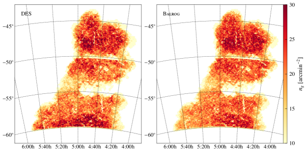
Figure 3: Map (declination vs. right ascension) of the density of detected DES (left) and Balrog galaxies (right) on the SPT-E footprint used in this analysis. While the two maps are very similar, there is an excess in counts in DES data at declination $\delta<-58$; this is due to increased stellar contamination caused by the nearby LMC. Our Balrog run has made no attempt to model anisotropic stellar counts.

The DES SV data were processed through the DES Data Management (DESDM) reduction pipeline (Mohr et al., 2012, Desai et al., 2012); we briefly outline salient reductions and refer readers to the references for further details. First, single epoch images are overscan subtracted, a cross-talk correction is made, and a look up table removes nonlinear CCD responses to incident flux levels. Bias frames are applied to subtract out any remaining additive offsets, dome flats correct for multiplicative variations in pixel sensitivity, and a “star flat” (e.g. Manfroid, 1995) divides out the illumination pattern across the detector. Artifacts such as cosmic rays, satellite trails, and stellar diffraction spikes are masked. Astrometric solutions are computed by scamp (Bertin, 2006) matching stellar positions to the UCAC4 reference catalog (Zacharias et al., 2013). The pipeline outputs reduced images, along with inverse-variance weight maps and masks.

DES’ photometric calibration is described in detail in Tucker et al. (2007). Briefly, SDSS photometric standards fields are observed at the beginning and end of each night. Stars from the DES images are matched to SDSS standard stars, fitting each band’s absolute zeropoint as a linear function of airmass over all overlapping matches. The zeropoint for each CCD in every image is then refit by jointly minimizing the magnitude differences between (1) DES objects common to multiple exposures and (2) any DES objects that match to SDSS standards.

DESDM builds coadds of the single-epoch images with SWarp (Bertin et al., 2002), using the discussed astrometric solutions and photometric calibrations as input. Each coadd image, known as a tile, is $\sim\!0.5~{}\mathrm{deg}^{2}$ in area. SWarp computes the effective gain noise level of each tile as well as the combined inverse-variance weight map. PSFEx (Bertin, 2011) is then run over the coadds to fit the PSF model, using a second-degree polynomial for interpolation over the tile. Finally, DESDM runs SExtractor in dual-image mode, using a multi-band $riz$ image for detection, to produce the catalogs of DES objects.

The SV photometric calibration for the coadds was supplemented with stellar-locus regression (SLR), which uses the near universality of the colors of Milky Way halo stars as a means to fit for photometric zeropoints (e.g. High et al., 2009). Our SLR corrections (Rykoff et al. in prep.) were implemented with a modified version of the big-macs stellar-locus fitting code (Kelly et al., 2014). All corrections were made relative to an empirical reference locus derived from calibrated standard stars observed on a photometric night. We recompute coadd zeropoints over the full SV footprint on a HEALPix (Górski et al., 2005) grid of NSIDE = 256, using bilinear interpolation to correct all objects in the catalog at a scale of better than $\sim\!14\arcmin$. We use $J$ band magnitudes from the Two Micron All Sky Survey (2MASS) stellar catalog (Skrutskie et al., 2006) as an absolute calibration reference, which yields absolute calibration uniformity of better than $2\%$, with color uniformity $\sim\!1\%$.

3.3 Running Balrog

The input we give to Balrog is made up of the data products discussed in the previous section: the coadded SV images from DESDM, as well as their inverse-variance weight maps, PSF models, astrometry, photometric zeropoints, and effective gains. We self-consistently add the same Balrog objects to the $g$, $r$, $i$, and $z$ images, build an $riz$ detection image for each realization using identical SWarp configuration as DESDM, and then run Balrog over each band with SExtractor configurations, which again match those of DESDM.

We make use of the SLR offsets introduced in Section 3.2 in our imaging simulations. We employ Balrog’s user-defined function API to read the SLR zeropoints and make position-dependent modifications to the simulated fluxes in each image, in addition the usual single zeropoint used by Balrog. This takes an input truth magnitude and adjusts it back to the pre-SLR flux scale, i.e. the original calibration for the coadd images.

In each Balrog realization we add only $1,000$ objects to the image (of area $\sim\!0.5~{}\mathrm{deg}^{2}$), in order to keep the Balrog-Balrog blending rate low. We iterate each coadd tile 100 times, simulating a total of 100,000 objects per DES coadd tile. Combining the results generates a Balrog output measurement catalog which is approximately the same size as the DES measurement catalog. The total run time for our Balrog simulations was approximately $30,000$ CPU-hrs, much less than the time needed by DESDM to process the data.

Admittedly, injecting our Balrog objects directly into the coadds instead of self-consistently into each overlapping single-epoch image is less ideal. For example, the coadd PSF is not as reliable of a model of the data as is simultaneously using the full set of single-epoch PSFs. However, the single-epoch version of Balrog is roughly ten times more computationally expensive, and we opt to test the simpler approach first. Using Balrog in other DES analyses which are more sensitive to the PSF and which directly use single-epoch level information (such as weak lensing ones) will require running on all the single-epoch images. In this work, our measurements are focused on galaxy clustering, and we demonstrate that the coadd approximation is sufficient in this context.

3.4 Catalog selection

Table 1: MODEST_CLASS selection.

Galaxies	Stars
(FLAGS_I $\leq 3$) AND NOT	(FLAGS_I $\leq 3$) AND
(   ((CLASS_STAR_I $>0.3$) AND (MAG_AUTO_I $<18$))	(    (CLASS_STAR_I $>0.3$)
OR ((SPREAD_MODEL_I + 3*SPREADERR_MODEL_I) $<0.003$)	AND (MAG_AUTO_I $<18$)
OR ((MAG_PSF_I $>30.0$) AND (MAG_AUTO_I $<21.0$))	AND (MAG_PSF_I $<30.0$)
)	OR (((SPREAD_MODEL_I + 3*SPREADERR_MODEL_I) $<0.003$) AND
	((SPREAD_MODEL_I + 3*SPREADERR_MODEL_I) $>-0.003$)))
	)

To construct the DES sample, we download the SV coadd data from the DESDM database of SExtractor measurements, returning detections from the same areas where Balrog was run. We then apply the SLR zeropoint shifts to both the DES and the Balrog catalogs. At this point, the full Balrog and DES catalogs total $\sim\!16$ million detections each.

Next, we apply some quality cuts to both samples. In Section 5, we undertake galaxy clustering measurements, and the quality cuts we make are similar to ones made in the benchmark DES clustering analysis of Crocce et al. (2015). We base our cuts on a subset of their selection criteria as means to help achieve a reasonably well-behaved source population.

First is a simple color selection:

$$-1 <\texttt{MAG\_AUTO\_G}-\texttt{MAG\_AUTO\_R}<3\;$$

$$\texttt{AND}\;\;-1 <\texttt{MAG\_AUTO\_R}-\texttt{MAG\_AUTO\_I}<2\;$$

$$\texttt{AND}\;\;-1 <\texttt{MAG\_AUTO\_I}-\texttt{MAG\_AUTO\_Z}<2.$$

This helps to eliminate objects inside regions which are contaminated in one filter band’s image, but not the others, such as satellite or airplane trails.

Furthermore, we make a cut based on SExtractor position measurements. Among the SExtractor detections, there exists a class of objects whose windowed centroid measurements are significantly offset in different filter bands, up to over a degree in the worst cases. This is to be expected for objects with low signal-to-noise ratios, since detection occurs in $riz$, while measurement occurs in each band independently, and the centroid measurement for a dropout in a given band is essentially unconstrained. However, large positional offsets persist at all signal-to-noise levels, such that about 2% of all objects at any signal-to-noise have significant offsets. We reject any object with large ($>1$″) offset between the $g$- and $i$-band centroids, which has been detected with $>5\sigma$ significance in $g$-band.

We also apply the mask used by Crocce et al. (2015). (Specifically, we use the mask as it exists prior to introducing redshift dependence.) The details of the mask’s construction are found in Appendix A; in brief, it is based on five criteria:

1. coordinate cuts to select SPT-E area north of the LMC,

2. excising regions with the highest density of large positional offset objects discussed above,

3. removing objects in close proximity to bright stars,

4. selecting regions with $10\sigma$-limiting magnitude of $i>22.5$, and

5. requiring detections over a significant fraction of the local area.

The cuts we have mentioned in this section are not strictly necessary for the validation tests presented in Section 4 to follow. In fact, Balrog is able to populate objects like the ones that have been cut into the simulated sample. However, we are most interested in Balrog’s behavior for objects which will survive into a science analysis. Therefore, we choose to exclude them from the clustering study presented in Section 5.

Throughout the remainder of our analysis, we also remove any objects from the Balrog simulation catalog which have a matched counterpart in the catalog generated by running SExtractor prior to inserting any simulated objects (cf. Section 2.3). Doing so removes approximately 1% of the Balrog catalog. Some of these objects are genuine Balrog objects, some are DES objects, and others are blends of the two, depending on the relative brightness of the input Balrog object compared to the DES object found in the image at the simulation location. This choice does have a small impact ($\sim\!1\%$) on the clustering: including the ambiguous matches effectively mixes some real galaxies into the randoms used for clustering, artificially suppressing the clustering signal; excluding the ambiguous matches has the opposite effect. We discuss this issue along with other fundamental limitations of the embedding simulation approach in Section 5.1.

The final selection mechanism we use is star-galaxy separation. Star-galaxy separation is accomplished with the MODEST_CLASS classifier, which is explained in e.g. Chang et al. (2015), and utilized in additional DES analyses such as Vikram et al. (2015) and Leistedt et al. (2015). The classifier has been tested with DES imaging of COSMOS fields. Table 1 lists the full MODEST_CLASS selection criteria. It incorporates SExtractor’s default star-galaxy classifier CLASS_STAR, which is based on a pre-trained neural network, as well as morphological information about how well the object resembles the PSF; for each object, SPREAD_MODEL measures a normalized linear discriminant between the best-fit local PSF model derived with PSFEx, and a slightly more extended model made from the PSF convolved with a circular exponential disk (see e.g. Desai et al., 2012, Bouy et al., 2013, Soumagnac et al., 2015). SPREADERR_MODEL is the error estimate for the SPREAD_MODEL measurement.

Including the cut on SPREADERR_MODEL, in addition to SPREAD_MODEL alone, improves the faint end galaxy completeness. Including the MAG_PSF cut improves the purity at the bright end. Soumagnac et al. (2015) investigate more sophisticated means of star-galaxy separation, such as machine learning techniques beyond SExtractor’s pre-trained CLASS_STAR, and in a subsequent publication (Aleksić et al. in prep.), we will present a neural network approach trained on Balrog data. In Section 5.5 we demonstrate that MODEST_CLASS suffices for our current analysis.

After applying all the cuts discussed in this section, the DES and Balrog galaxy catalogs total $\sim\!10$ million objects each. These are the samples whose number densities we mapped in Figure 3. We use these catalogs as our primary data products in Section 4 and Section 5.

4 Balrog Validation

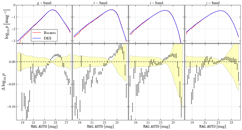
Figure 4: Top: Magnitude distributions (PDFs) of DES and Balrog galaxies in four DES filters. Bottom: Illustration of the difference between DES and Balrog magnitude distributions is shown in black; errors are estimated from jackknife resampling, as described in Appendix B. The yellow band shows the sample variance of the DES catalogs, also jackknife estimated.

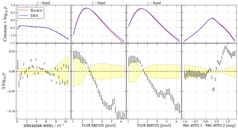
Figure 5: Top: An idiosyncratic selection of measured photometric properties. The logarithmic PDFs for DES and Balrog in each panel have been shifted by an additive constant. From left to right: reported errors in one of SExtractor’s stellarity measures, $i-$band size, $z-$band size, and $i-z$ color. We expect the filter mismatch described in Section 3.1 to drive at least some of the color residuals. Cosmic variance in the COSMOS field is also present, though we have made no rigorous attempt to estimate its impact here. Bottom: analogous to Figure 4; in black, we show the difference between the DES and Balrog distributions in the top panel. The yellow band indicates the sample variance of the DES measurements. All errors are estimated from jackknife resampling. (See Appendix B for further details.)

To validate Balrog’s functionality, we analyze the catalogs constructed in Section 3.4, testing if the properties of the Balrog objects are representative of the DES data. For our Balrog runs, we have attempted to build an input catalog which is deeper than our actual DES data. If this input distribution is indeed an adequately representative sample, and our DES calibrations (PSF, flux calibration, etc.) are well measured, running the simulations through Balrog should successfully reproduce measurable properties of the DES catalogs.

The Balrog and DES comparison tests presented in this section are as follows: Section 4.1 plots one-dimensional distributions of measured SExtractor quantities, Section 4.2 does similarly for two-dimensional distributions, and Section 4.3 considers number density fluctuations. Section 4.2 and Section 4.3 include assessments of the populations’ behavior as a function of observing conditions of the survey. The one- and two-dimensional distributions offer a general overview of the agreement between Balrog and DES, and the number density tests validate that the agreement is sufficient to use our Balrog galaxies as randoms in Section 5’s clustering measurements.

We also make note of Appendix B, where we explain our jackknifing procedure, used to estimate errors in this section, as well as in Section 5. To summarize, we use a $k$-means algorithm to separate our data sample into 24 spatial regions of roughly equal cardinality, then leave one region out in each jackknife realization and calculate the covariance over the realizations.

4.1 One-dimensional distributions

We compare the $griz$ magnitude (MAG_AUTO) distributions of galaxies, for both the DES and the Balrog samples in Figure 4. The top row of the figure plots each band’s $\log_{10}p$, the logarithm of the PDF, and the second row plots the difference in this quantity between Balrog and DES, i.e. the fractional deviation between the two PDFs. The error bars plotted are the square root of the diagonal elements of the jackknife covariance matrix, as described in Appendix B, where we have jackknifed the difference curve, $\Delta\log_{10}p$. For MAG_AUTO $\gtrsim 21$ – the region of the parameter space occupying the bulk of the galaxies – Balrog reproduces the DES distribution to better than 5% differences, approaching 1% over some intervals. The yellow bands in bottom row of Figure 4 show the jackknife errors of the DES PDFs plotted in the top row. In the densest parameter space regions, many of data points of the differences between Balrog and DES are within the DES variance, particularly in the $i$ and $z$-bands. This means that in these regions of magnitude space, Balrog galaxies are statistically indistinguishable from DES galaxies.

We also make plots analogous to Figure 4, using measured quantities other than single-band magnitudes (Figure 5). In each of the top panels, we have shifted $\log_{10}p$ for both the DES and Balrog curves by an additive constant, so all the panels share a similar range on the $y$-axis. We plot distributions in (MAG_AUTO_I - MAG_AUTO_Z) color, $i$-band SPREADERR_MODEL, as well as $i$- and $z$-band FLUX_RADIUS. FLUX_RADIUS measures the PSF convolved half light radius. SPREADERR_MODEL is the error in the SPREAD_MODEL measurement introduced in Section 3.2. We again find that Balrog reproduces DES to $\sim$$\,5\%$ differences or better in the bulk of the distributions; this result holds across bands and across different SExtractor quantities. We chose to include SPREADERR_MODEL in our comparison because it is not obviously straightforward to simulate directly; it is the error in a measurement unique to SExtractor. Nevertheless, Balrog is able to recover a distribution similar to DES.

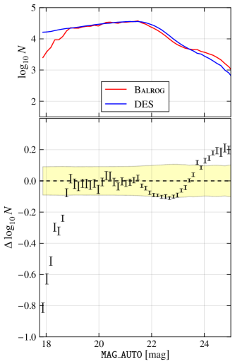
Figure 6: Stellar magnitude distributions in DES and Balrog, $i$-band. The Balrog curve has been normalized by selecting $23<\texttt{MAG\_AUTO\_I}<24$ objects, and multiplying by the detected DES star-to-galaxy number ratio divided by the detected Balrog star-to-galaxy number ratio (as in Section 5.5 when estimating DES stellar contamination levels). At the bright end, the difference is primarily a result of the lack of bright stars ($i<19$) in the CMC catalog (due to saturation in the COSMOS images) used to seed the Balrog simulations. Furthermore, the stellar density varies substantially across the SV field (see Figure 12), so the COSMOS stellar population is not necessarily representative.

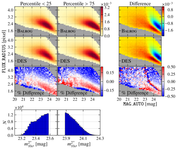
Figure 7: Top left block: These six panels show the sensitivity of the $i$-band size-magnitude distributions of DES and Balrog galaxies to survey depth. The color scale in the upper four panels shows normalized counts. Bottom block: Histograms of the depth selection in each column; we split into two samples: the deepest 25% of the area and the shallowest 25% of the area. Right block: Differences between the left panels. The bottom panel shows the difference between the above two differences. While these histograms are noisy, this figure shows that Balrog well captures the effect of depth on the measured galaxy properties. The systematic differences visible here are mainly due to the small differences between the DES and CMC catalogs.

If Balrog were a perfect model of the data, $\Delta\log_{10}p$ would be consistent with zero everywhere, but in practice, we do not expect to recover this result. Even in the limit of perfect survey calibrations (PSF, photometric calibration, etc.), one would need a completely representative input population to recover perfect agreement. We have made the assumption that single component elliptical Sérsic objects fully describe the galaxy population, but this is not strictly true. Moreover, COSMOS (point) sources begin saturating for $i\lesssim 19$ (Leauthaud et al., 2007, Capak et al., 2007). The CMC does not include such objects, and thus our reweighted catalog is not expected to be entirely complete at bright magnitudes. Furthermore, COSMOS is a small field ($\sim\!2~{}\mathrm{deg}^{2}$): with limited statistics and cosmic variance, it is not necessarily entirely representative of a larger area survey like DES, especially at brighter and larger size limits; this could be another contributing factor why Balrog’s brighter and larger galaxies are less representative of DES than its fainter and smaller ones. Finally, we have also used Subaru filters for our input magnitudes, (because DECam ones were not available), which will introduce some error when comparing Balrog and DES distributions.

Figure 4 and Figure 5 plotted galaxy selections, but our Balrog run also included stars. Figure 6 shows the $i$-band DES and Balrog stellar distributions. We have normalized the Balrog curve in the top panel in the following way: $N$ in each bin of the Balrog curve is multiplied by the detected star-to-galaxy number ratio in DES divided by the detected star-to-galaxy number ratio in Balrog, where we have selected detections from $23<\texttt{MAG\_AUTO\_I}<24$. (This is the same way we normalize when estimating the DES stellar contamination ratio of our faint clustering sample in Section 5.5.)

There is more variation in the stellar distributions compared to the galaxy distributions, and this is to be expected. First, we see a large deficit due to the effects of saturation in the COSMOS imaging at $i\lesssim 19$, as mentioned above. Stars are more compact than galaxies and thus more heavily affected by saturation. Furthermore, the stellar population intrinsically fluctuates much more strongly across the sky than the galaxy population, and the small stellar sample from the COSMOS field need not be entirely representative of DES as a whole. Indeed, the DES catalog contains more detected stars than the Balrog catalog.For this analysis, we are primarily interested in galaxies and the COSMOS stellar population suffices; however, in a broader context, we offer it as an example of how one should be mindful to use Balrog with an input simulation population which is appropriate for one’s science case.

4.2 Two-dimensional distributions and observing conditions

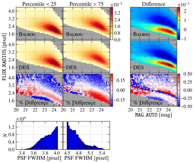
Figure 8: Analogous to Figure 7, but instead showing the ($i$-band size-magnitude) dependence on average seeing in the coadd images. Again, Balrog successfully captures the dependence of the measured galaxy properties on observing conditions. The systematic differences visible here are mainly due to the small differences between the DES and CMC catalogs.

In addition to validating Balrog’s ability to recover DES’ distributions of measured quantities, we also need to test if Balrog behaves like DES as a function of observing properties of the survey. Leistedt et al. (2015) have constructed HEALPix maps of several characteristics of the DES SV observations, including PSF full width at half maximum (FWHM), 10$\sigma$ limiting magnitude in 2″ apertures ($m_{10\sigma}^{2^{\prime\prime}}$), airmass, sky brightness, and sky variance (where the square root of sky variance is called sky $\sigma$). Each map computes an average of a given quantity in the overlapping single-epoch observations for any pixel in the map, using either an ordinary mean or a weighted mean, where the weights are taken from the single-epoch inverse variance maps. We use the maps of Leistedt et al. (2015), available at a resolution of $\texttt{NSIDE}=4096$, and compare Balrog’s behavior against DES’ behavior as a function of the observing conditions.

First, we split our DES and Balrog galaxy samples into two divisions according to the local 10$\sigma$ magnitude limit, selecting the top and bottom 25 percentiles. The depth histograms for these two samples are shown in the bottom row of Figure 7, with the shallower sample in the left column. The first two rows of this leftmost column show normalized Balrog and DES two-dimensional histograms in the $i$-band size-magnitude plane for the shallower magnitude limit selection. The top two rows of the middle column show likewise for the deeper selection. The third row quantifies the fractional difference between the Balrog and DES rows. Like the one-dimensional examples, in the densest regions of parameter space Balrog and DES largely agree. Moreover, simultaneous agreement in both depth samples offers evidence that Balrog traces the distribution’s properties as a function of magnitude limit. The rightmost column of Figure 7 further tests this: the top two rows in this column plot the Balrog and DES differences of the shallower and deeper distributions, and the third row plots the fractional difference between the two rows above, i.e. this panel compares the DES and Balrog magnitude-size derivative with respect to magnitude limit. Except in regions of sharp change, agreement in well-sampled areas of parameter space is typically $\sim\!10\%$ differences, offering additional evidence that Balrog reasonably tracks the DES changes with observing conditions.

We have made analogous plots to Figure 7, splitting on properties other than magnitude limit, and find similar results. Figure 8 offers another example, dividing the sample based on PSF FWHM. The figure is largely reminiscent of Figure 7.

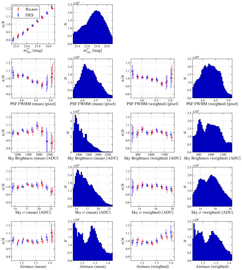
Figure 9: Number density fluctuations in the DES and Balrog galaxy samples as a function of $i$-band survey properties, binning the survey properties over the 2 to 98 percentile range. (The DES and Balrog curves have been slightly offset for visual clarity.) For each number density bin, we count the number of galaxies in the given pixels, divide by the area covered by those pixels, and normalize by the average density over the full sample. Error bars are estimated from 24 jackknife resamplings of the curves (cf. Appendix B). Alongside the number density plots are histograms of the survey observing conditions, again binned over the 2 to 98 percentile range.

4.3 Number density and observing conditions

To conclude this section, we test Balrog’s ability to recover DES-like number density fluctuations as a function of the survey properties mapped by Leistedt et al. (2015), i.e. we investigate if Balrog recovers DES’ window function over the observing conditions. If this check is successful, it means Balrog galaxies can be used as a set of random points in a clustering analysis in order to correct for varying detection probability over the footprint. In Section 4.1 and Section 4.2, we demonstrated that Balrog is largely, but not perfectly, representative of the DES data; assessing whether or not agreement is good enough depends on one’s science case. Here, we investigate if the agreement is at an adequate level such that Balrog detection rates are representative of DES detection rates, within the respective error estimates.

Figure 9 plots number density fluctuations in our full DES and Balrog galaxy samples as a function of $i$-band survey properties, binning in each survey property over the 2 to 98 percentile range. Alongside these number density plots, we also include the histograms of the survey observing conditions over the same range. For each number density bin, we count the number of galaxies in the given pixels, divide by the area covered by those pixels, and normalize by the average density over the full sample. We plot both the DES and Balrog samples, where the points have been slightly offset for visual clarity. The error bars on each set of points are estimated by 24 jackknife realizations of the curve, as described in Appendix B. We find that the DES and Balrog results are consistent with each other within the errors estimates, which demonstrates Balrog’s modeling as adequate to recover the DES window function over the tested sample. We have repeated this exercise using the survey properties across other filter bands, finding consistent results.

5 Angular Clustering

The final test of the Balrog catalogs described in this paper is their use in systematic error amelioration for an angular clustering measurement. Selecting the Balrog catalog in the same way as the real catalog produces a sample with a nearly identical window function as the data’s. The Balrog catalogs have inherited systematic errors in the imaging and analysis pipelines, but otherwise have no intrinsic clustering themselves. Hence, using them as randoms in a two-point estimator is a simple and efficient way of removing the systematic errors while maintaining the real clustering signal. The rest of this section describes how this is done.

We describe what we believe are the practical and fundamental limitations of embedding simulations for clustering measurements in Section 5.1. Section 5.2 discusses the algorithms we use to make our $w(\theta)$ measurements. In Section 5.3, we select two magnitude-limited DES samples and perform tests in Section 5.5 to show that stellar contamination is unimportant for the measured angular clustering signals. In Section 5.4, we select similar populations from the public COSMOS galaxy catalog of Capak et al. (2007) ($\sim\!2~{}\mathrm{deg}^{2}$ in area) and match them to our DES samples. Section 5.6 then demonstrates that over the measurable range of angular separations, our Balrog-corrected DES measurements reproduce the much deeper COSMOS measurements, but with substantially improved accuracy and range, owing to the larger survey volume. The shapes of our $w(\theta)$ results follow model predictions.

5.1 Caveat Likelihood

Fundamentally, our simulated galaxies are sampling the likelihood function that connects the measured parameters ($\bm{\alpha}_{\rm meas}$) of stars and galaxies to the underlying true parameters ($\bm{\alpha}_{t}$) of objects in the DES images. In general, the detection probability and measurement biases for some particular galaxy depend on the rest of the galaxies in the image, even including objects that may not be detected. Denoting the set of all relevant object parameters by $\{\bm{\alpha}\}$, and expressing the dependence on position on the sky $\bm{\theta}$ explicitly, we can write:

$$\mathcal{L}=p(\bm{\alpha}_{\rm meas}\>|\>\left\{\bm{\alpha}_{t}\right\},\bm{\theta}).$$ (2)

$\mathcal{L}$ is meant to incorporate sample selection criteria, so the probability $p(\bm{\theta})$ of any object being selected for analysis is the likelihood integrated over the true and observed properties:

$$p(\bm{\theta})=\int\>p(\bm{\alpha}_{\rm meas}\>|\>\left\{\bm{\alpha}_{t}\right\},\bm{\theta})\>d\bm{\alpha}_{\rm meas}d\{\bm{\alpha}_{t}\}.$$ (3)

This is also sometimes called the window function, and it is this function that the random catalogs used in correlation function estimators (like Equation 6) are meant to be sampling.

The likelihood sampled by the Balrog catalogs is only an approximation of the true $\mathcal{L}$. In part, this is a result of simplifications made in the simulation. Our input catalog, for instance, is limited in its realism by the galaxy templates used to generate the synthetic colors in the COSMOS mock catalogs and by the finite size of the COSMOS field. This limitation is equivalent to integrating in Equation 3 only over the regions of $\bm{\alpha_{t}}$ covered by COSMOS. This issue is one of several described above that can in principle be addressed with improvements to the simulations.

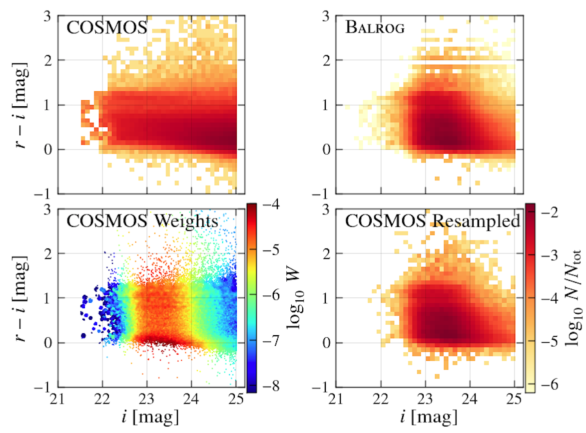
Figure 10: COSMOS sample selection. The heat map colored histograms plot normalized counts. Top left: $i$-band magnitudes and $r-i$ colors for the full COSMOS catalog after basic quality cuts. Top right: Distribution of $i$-band magnitude and $r-i$ colors using truth catalog properties of Balrog galaxies in our faint sample. Bottom left: (Unnormalized) weights applied in the $i$, $r-i$ color plane to COSMOS galaxies in order to match the DES truth distribution. Bottom right: $i$-band magnitudes, $r-i$ colors of the reweighted COSMOS sample.

There are more fundamental limitations to this procedure, however. When a simulated galaxy and a real galaxy overlap, it is not always possible to determine whether the resulting catalog entry belongs in the Balrog catalog. If the real object is largely unmodified by the presence of the simulated galaxy, then associating it with the truth properties of the simulated galaxy results in an incorrect measurement of $\mathcal{L}$. If the real object is substantially modified by the presence of the simulated galaxy, the resulting catalog entry could be used to infer the likelihood function for blends, though we have not built the inference machinery necessary to do so. Finally, if the simulated object’s properties are not substantially modified by the presence of the real object, then associating the resulting catalog entry to the simulated object’s truth properties results in a useful measurement of $\mathcal{L}$ at that location.

These ambiguous matches tend to introduce a small amount of real galaxy contamination into the randoms, and result in a small multiplicative bias to the clustering of roughly twice the contamination rate. Excluding them excludes some Balrog galaxies in a manner that reverses the sign of the multiplicative bias, with similar amplitude. Ambiguous matches comprise only $\sim$$\,1\%$ of our Balrog galaxies, resulting in a multiplicative bias that is smaller than the statistical error on the amplitude of the $w(\theta)$ measurement presented below. For this reason, we do not apply any correction for this effect.

Finally, and most fundamentally, Balrog samples the likelihood under slightly different conditions than the real data. If the image contains $n$ real objects, the measurement likelihood for the $n^{th}$ is

$$\mathcal{L}=p(\bm{\alpha}_{n,\rm meas}\>|\>\bm{\alpha}_{t,1},\bm{\alpha}_{t,2},...,\bm{\alpha}_{t,n-1},\bm{\theta}),$$ (4)

while the likelihood sampled in this image by a single added Balrog galaxy is:

$$\mathcal{L}=p(\bm{\alpha}_{n+1,\rm meas}\>|\>\bm{\alpha}_{t,1},\bm{\alpha}_{t,2},...,\bm{\alpha}_{t,n-1},\bm{\alpha}_{t,n},\bm{\theta}).$$ (5)

If the likelihood really is strongly non-local – that is, if the measured properties of each galaxy depend strongly on the properties of other nearby objects – then the Balrog catalogs will not be sampling the same likelihood as the data, and we should not expect $w(\theta)$ estimates made with them to be correct. All correlation function estimators that use random catalogs assume that the window function and the density field are statistically independent, however, so a coupling between $\mathcal{L}$ and the galaxy density field would also make Equation 6 invalid for any random catalog.

These complications should all be much less severe for catalogs made with the high-resolution space-based COSMOS imaging. Insofar as this is true, we can regard any measured difference between the COSMOS angular clustering and that measured with Balrog as evidence that the simulated catalogs are not sampling the same likelihood function as the data.

5.2 Estimation algorithms

We adopt the Landy & Szalay (1993) estimator for the correlation function:

$$w\!\left(\theta\right)=\frac{DD-2DR+RR}{RR},$$ (6)

with $D$ labeling the data and $R$ labeling the randoms. The randoms sample the window function for an intrinsically unclustered sample, and are used to remove any signal induced by non-uniform detection probability. For our DES data, we will compare estimates of $w(\theta)$ made using Balrog randoms to the same measurements using uniform randoms that sample the survey geometry only (by applying the same spatial masking to the uniform randoms as applied to the data). We have not run Balrog on the COSMOS imaging, and hence all our COSMOS $w(\theta$) measurements use the standard uniform randoms.

We compute Equation 6 using TreeCorr (Jarvis et al., 2004), a software package implementing a $k$-d tree algorithm for efficient calculation of correlation functions over large datasets. We adjust the bin_slop parameter, which controls the fraction of the bin width by which pairs are allowed to miss the correct bin, such that $\texttt{bin\_slop}\times\texttt{bin\_size}<0.1$, in order to reduce the binning errors made by the algorithm. We run TreeCorr over each of the 24 $k$-means jackknife realizations, as explained in Appendix B, in order to estimate the correlation function’s covariance.

As a cross-check, we have also computed our correlation functions with athena (Schneider et al., 2002), another tree-code which implements its own internal jackknife algorithm to estimate the covariance, where the data’s area is divided into squares on a grid of $N$ rows $\times$ $M$ columns, leaving out one of the squares in each jackknife iteration. Using either code, we measure consistent $w(\theta)$ signals.

As discussed in Crocce et al. (2015), jackknife resampling is a noisy estimate of the covariance of $w(\theta)$, which is reasonably well-suited for the diagonal elements, but theory-based errors are better-suited for the off-diagonal terms. Because we attempt no physical interpretation of our clustering signals, we omit any theoretical modeling, and do not explore noise estimates beyond jackknife resampling.

5.3 DES sample selection

We choose two separate DES samples for our clustering measurements: a bright sample ($21<\texttt{MAG\_AUTO\_I}<22$), which is a subset of the magnitude selection used in the DES benchmark clustering analysis of Crocce et al. (2015), and a faint sample ($23<\texttt{MAG\_AUTO\_I}<24$), where the DES catalogs are substantially incomplete, and, as we will see in Section 5.6, the variation in the observed galaxy density across the sky is dominated by variations in the selection function. We should expect the bright clustering signal measured with Balrog randoms to easily reproduce the signal measured with uniform randoms (as done in the DES benchmark clustering analysis) and to agree with COSMOS; this is primarily a sanity check. Our faint selection is a strong test of the methodology – success here would indicate accurate measurement of spatial clustering even where, because of the low signal-to-noise ratio of the sample, anisotropies in the window function strongly affect the intrinsic clustering signal. Neither sample is identical to the DES benchmark sample; in Appendix C we offer a brief look at this sample.

5.4 COSMOS sample selection

We use the public COSMOS multi-wavelength photometry catalog (Capak et al., 2007) to validate our clustering measurements. First, we make a few basic quality cuts, selecting objects with:

blend_mask = 0

AND star = 0

AND $$\texttt{auto\_flag > -1}.$$

At the time of this writing, we did not have an appropriate angular mask for the COSMOS field. We have used the positions of objects flagged as problematic in the COSMOS photometric catalog as our mask definition. When constructing our sample, we first exclude any COSMOS galaxy within $10\arcsec{}$ of an object flagged as bad. Visual inspection shows good agreement between this set of bad objects and problematic regions in the COSMOS imaging. Unfortunately, this shortcut makes the small-scale COSMOS clustering difficult to interpret, so we elect not to use COSMOS measurements of $w(\theta)$ for $\theta<10\arcsec{}$ in the analyses. We have increased the 10″ separation cut, and verified that our results on scales larger the masking radius are not sensitive to the value chosen.

Small changes in the properties of the selected galaxies can have significant effect on the amplitude of $w(\theta)$, so we take care to ensure that the sample we select from COSMOS is well-matched to the DES galaxies. Our technique for doing this is a resampling scheme based on and motivated by that described in e.g. Lima et al. (2008), Sánchez et al. (2014), and analogous to how we reweighted our Sérsic catalog in Section 3.1.

First, we make the same cuts on the Balrog galaxies as we have for the DES galaxies (cf. Section 5.3). For each Balrog galaxy, we also have the truth magnitudes and colors used to generate the galaxy, which are directly comparable to the magnitudes and colors from the COSMOS photometric catalog (cf. Section 3.1). Matching the properties of the Balrog and COSMOS catalogs in this space should ensure similar samples with comparable clustering. We choose to work in two dimensions: $i$-band magnitude and $r-i$ color, selecting i_mag_auto and ($\texttt{r\_mag}-\texttt{i\_mag}$) from the COSMOS catalog as the complements to our Balrog truth quantities. The top row of Figure 10 presents the COSMOS measurements alongside our faint Balrog selection for the chosen quantities.

To match the samples, for each COSMOS galaxy we calculate the distance to the $50^{\rm th}$-nearest Balrog galaxy in this color-magnitude space. The number of COSMOS galaxies inside this distance is proportional to the ratio of the two distributions, and when properly normalized, equal to the weight required to match them. Normalization is such that the ensemble of weights sums to unity. We then randomly resample the COSMOS catalog, using the calculated weights as the selection probability for each object, which generates our DES-matched COSMOS sample.

We repeat this process separately for both the bright sample and the faint sample; Figure 10 presents our results for the faint sample. Using the weights in the bottom left panel, we resample the COSMOS catalog in the top left panel. After doing so, we recover the bottom right panel, which is a good match to the top right panel – the faint Balrog sample. We have confirmed that, after this matching, the $g-$ and $z-$band magnitude distributions are also strikingly similar to the Balrog truth distributions. We have also matched on quantities other than $r-i$ color and $i$-band magnitude, as well as varied the number of nearest neighbors to query, and measured consistent clustering signals.

5.5 Stellar contamination

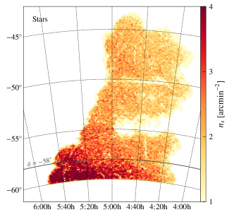
Figure 11: Map (declination vs. right ascension) of the DES stellar number density across the SPT-E footprint. An additional parallel has been drawn at $\delta=-58\degr{}$, indicating the cut we make in our clustering measurements to eliminate the area of highest stellar contamination.

Stars that are accidentally included in the galaxy clustering analysis can have a significant impact on the measured clustering (e.g., Scranton et al., 2002, Maddox et al., 1996). An unclustered stellar population simply dilutes the measured angular clustering. If the stars themselves cluster nontrivially, the measured signal is a mixture of the true galaxy and stellar clustering, with mixture coefficients set by the fraction $f$ of the galaxy sample that has been mis-classified as stars. We refer readers to Appendix D of Crocce et al. (2015) for a detailed treatment of the subject.

To estimate the stellar contamination in our DES samples, we use the Balrog simulations. From the Balrog truth catalog, we can infer the fraction of Balrog objects which were simulated as stars but misclassified as galaxies. However, because the DES and Balrog stellar densities vary (cf. Section 4.1), we need to renormalize this Balrog contamination rate; we multiply by the detected DES star-to-galaxy number ratio and divide by the detected Balrog star-to-galaxy number ratio.

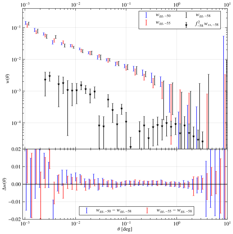
Figure 12: Testing stellar contamination. All error bars in the figure are estimated with jackknife resampling (cf. Appendix B). Top: The bar-only points show galaxy angular correlation function measurements for our faint ($23<\texttt{MAG\_AUTO\_I}<24$) DES sample over different declination ranges: $\delta>-50$ in blue, $-55<\delta<-50$ in red, and $-58<\delta<-55$ in black. (For visual clarity, only every other point has been plotted, and there is a slight offset between points at the same angular scale. Legend labels denote the southern edge of the regions.) Stellar density varies between the regions (cf. Figure 11), and a stellar contamination dilution correction has been applied to each curve (cf. Section 5.5). The contamination fractions for each region are: $f_{-50}=0.044$, $f_{-55}=0.048$, $f_{-58}=0.058$. The black stars plot the stellar autocorrelation function multiplied by the square of the galaxy stellar contamination fraction, in the region of highest stellar density and highest stellar clustering. (To maintain readability, we omit the stellar autocorrelations over the other two regions, and choose to focus on the most pessimistic case.) If large enough, the stellar autocorrelation quantity can induce an additive bias to the galaxy clustering measurements, and we note that it is comparably small over the range of scales where we are able to make a statistically significant measurement. Bottom: Differences between the stellar contamination dilution corrected galaxy autocorrelation function measurements in the top panel. There is no significant difference between the resulting measurements, suggesting that stellar contamination is not a significant source of systematic bias for this measurement.

In both the bright and faint DES samples, we find $f\sim\!5\%$. Inspection of the magnitude-FHWM plane in the COSMOS data indicates that stellar contamination is small ($\sim\!0.1\%$ for $i<22$), so we omit any corrections due to this contamination in the COSMOS measurements.

As shown in Figure 11, the stellar density varies dramatically across the DES survey area examined in this analysis. The edge of the LMC intrudes at $\delta<-58$, so we have removed this extreme region from the clustering analysis, and for the following tests we divide the remainder of the area into three declination-selected strips:

1. $\delta>-50$,

2. $-55<\delta<-50$,

3. $-58<\delta<-55$,

in order to test if our clustering signals are robust against stellar population size. The two northernmost regions are roughly equal in stellar density, while the southernmost’s is about 35% greater.

We measure the stellar autocorrelation $w_{ss}$ in each of the declination-selected samples. The expected spurious clustering from stellar contamination is proportional to this signal, but suppressed by the square of the contamination fraction (Myers et al., 2006, Crocce et al., 2015). We find that $f^{2}w_{ss}$ is well below errors in the angular correlation function for both the bright and faint samples; the faint measurements, which have larger stellar clustering, as well as slightly higher stellar contamination, are shown in Figure 12. (For visual clarity, Figure 12 only plots $f^{2}w_{ss}$ in the southernmost region, the most pessimistic case). To account for dilution from stellar contamination, we apply a $(1+f)^{2}$ correction (Myers et al., 2006, Crocce et al., 2015) to the galaxy autocorrelation functions. We show in the bottom of Figure 12 that after applying the correction, the differences between the galaxy signals for the three regions are small compared to the autocorrelation errors, further indicating that stellar contamination is not a significant source of systematic bias.

5.6 Clustering measurements

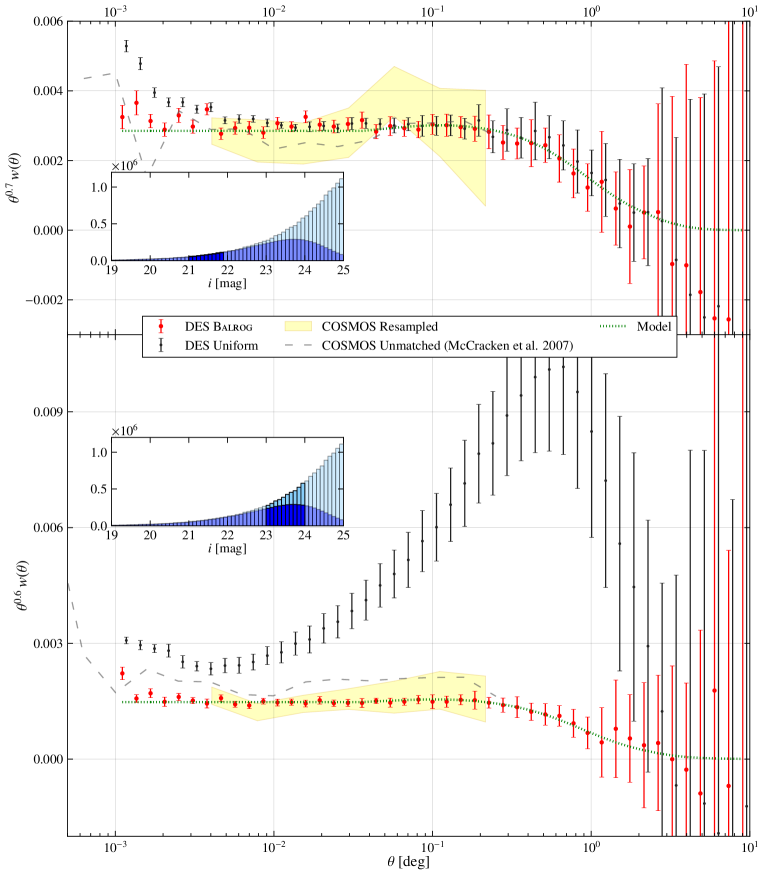
Figure 13: Angular clustering results. Black and red points show $w(\theta)$ measurements for our DES galaxies, with uniform and Balrog randoms, respectively. (Points at the same separation have been slightly offset for visual clarity.) The yellow band measures the 1$\sigma{}$ confidence interval on $w\!\left(\theta\right)$ in a matched COSMOS sample (cf. Section 5.4). All errors are estimated with jackknife resampling, (see Appendix B). The gray dashed lines are COSMOS measurements from McCracken et al. (2007), which we note are not matched to the DES sample, but which could be measured to a smaller scale than our DES-matched COSMOS measurements. (See Section 5.4 and Section 5.6 for more details). Dashed green lines are $\Lambda$CDM model predictions, not fits to the data (cf. Section 5.6). Insets show the distribution of true Balrog (light blue) and observed DES (blue) magnitudes, with selection regions highlighted. In both panels, we have multiplied the signal by its approximate power-law slope. Top: Clustering of the bright, fairly complete sample. As expected, variations in the DES window function, as measured by the Balrog randoms, do not appear significant for the clustering above $15$″ ($0.004\degr$). Bottom: Clustering of the faint sample, which is near or at the magnitude limit of the survey, and $\sim\!35\%$ incomplete on average. It is strongly impacted by systematic effects due to the spatial variations of DES survey properties. We include the measurement using uniform randoms purely as an estimate of the of the importance of systematic errors, noting that it would be inappropriate to use uniform randoms to measure $w\!\left(\theta\right)$ for a $23<i<24$ sample selected with 10$\sigma$ limiting magnitude $i>22.5$. The Balrog randoms appear to capture essentially all of the extra power, suppressing it by roughly two orders of magnitude (see Section 5.6 for further explanation). Note the excellent agreement with the matched COSMOS measurements. Like McCracken et al. (2007), Balrog suggests little deviation from a power-law down to small scales. The shape of Balrog results also agree with the shapes of the models.

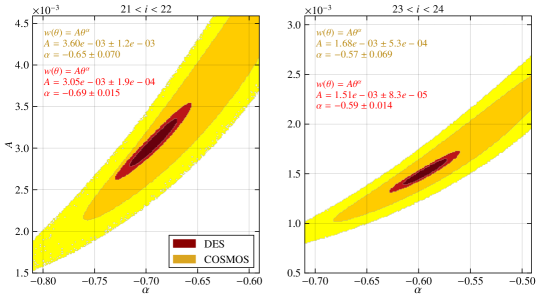
Figure 14: MCMC power-law fits for the $w(\theta)$ measurements shown in Figure 13. Contours are the 68% and 95% intervals. The DES measurements (red) use Balrog randoms, and the COSOMS measurements (yellow) are for the sample matched to DES. The text displays the best-fit marginalized parameter values. Left: bright sample. Right: faint sample.

We now present our $w\!\left(\theta\right)$ measurements. Angular clustering measurements for flux-limited samples generally see power-law behavior at small angular separations, steepening above degree scales (e.g. Maddox et al., 1996, Scranton et al., 2002, McCracken et al., 2007). We expect that significant residual additive systematic errors should produce a deviation from a constant power-law behavior below degree scales, while residual multiplicative biases should produce a corresponding multiplicative offset between the DES and COSMOS measurements.

Our bright sample galaxies are a subset of the DES benchmark sample, which has been extensively studied in a separate analysis (Crocce et al., 2015). The limiting magnitude of the benchmark sample ($i<22.5$) was made, in the conservative tradition of large-scale structure measurements, in order to produce a clean sample with relatively uniform selection; as shown in Figure 13, this selection indeed produces a reliable clustering signal at large scales.

The top panel of Figure 13 shows measurements of the angular clustering for our bright ($21<i<22$) sample. We plot $w\!\left(\theta\right)$ estimated using Balrog randoms in red, and that estimated using the uniform randoms in black. An overall correction to the amplitude of both these DES curves has been applied in order to correct for the effects of stellar dilution (cf. Section 5.5). The shaded region shows the $1\sigma$ confidence interval (inferred from jackknife resampling, cf. Appendix B) from the matched COSMOS photometric sample.

These three estimates are statistically consistent with one another within the range probed by our COSMOS clustering measurement. Any excess systematic power traced by the Balrog catalogs here is evidently not significant for the measurements above $\theta\gtrsim 15\arcsec$ ($0.004\degr$). Below this scale, the uniform and Balrog curves diverge; the measurements made using the Balrog sample continue the power-law behavior down to $\sim\!7^{\prime\prime}$, where blending effects start to become significant. We have not attempted to diagnose this behavior in detail. However, we remark that COSMOS measurements made by McCracken et al. (2007) for a similar, but not identical sample, also suggest little deviation from a power-law down to these scales; we include their measurements with our results in Figure 13. They select the same range of $i$-band magnitudes, but we note that the sample is not reweighted to match the DES one (cf. Section 5.4), and thus need not exhibit an identical signal. Therefore, the McCracken et al. (2007) results offer strong evidence, but not definitive proof, to validate the small-scale power-law-like Balrog results.

Our faint sample ($23<i<24$) is close to the formal limiting magnitude for the survey. As is evident from Figure 4, DES is substantially incomplete in this regime, and this is where we should expect the spatial variation in survey properties to matter the most. We include the clustering signal measured using uniform randoms purely as an estimate of the of the importance of systematic errors for this faint sample.

The bottom panel of Figure 13 presents our angular clustering results for this faint selection. Balrog and the faint-sample matched COSMOS results are in excellent agreement, and the former continues its power-law behavior down to almost $4\arcsec{}$ (0.001°). Subject to the same caveats discussed above, we again plot a COSMOS measurement from McCracken et al. (2007), using an unmatched sample over the same magnitude range, noting similar power-law behavior down to small scales.

The amplitude of the signal in the faint clustering measurement closely follows our COSMOS signal. We note that the systematic error has a substantially different shape than the galaxy autocorrelation, and so where it is significant, it should produce a deviation from the power-law behavior. This suggests that the residual additive systematic error in the faint sample Balrog measurement is small compared to the latter’s jackknife errors. At $0.5\degr$, the Balrog clustering errors are $\sim\!0.0005$, and so the spurious clustering has been suppressed by about two orders of magnitude from its value ($\sim\!0.01$ at the peak of the gray curve in Figure 13).

To show that the shape of our clustering measurements matches general expectations, we have included model $w(\theta)$ curves – the dotted green lines in Figure 13 – for $\Lambda$CDM cosmology ($\sigma_{8}=0.8$, $\Omega_{m}=0.31$). These have been generated assuming the broad $dN/dz$ used in Nock et al. (2010), Ross et al. (2011a) for a DES-like selection of galaxies. For separations $r>10$ Mpc/h, we use a linear-theory correlation function, $\xi(r)$, derived by Fourier transforming the CAMB (Lewis et al., 2000) power spectrum, with $\xi(r)\propto r^{-\gamma}$ for $r<10$ Mpc/h. Projection to angular separations follows Equations 9-13 in Crocce et al. (2011). $w(\theta)$ was scaled by an arbitrary factor, to account for galaxy bias and the true underlying dN/dz (both of which are expected to have nearly constant proportional effects on the amplitude as a function of $\theta$), with the curve set to be a power-law at $\theta<0.03\degr$. In Figure 13, the shapes of the measured $w(\theta)$ curves indeed trace those of the model predictions. In follow-up work, we will assess the impact on cosmological parameter sensitivity using our new methodology. Here, the uncertainties in $w(\theta)$ at large angular scales, where cosmological sensitivity is the greatest, are too large for us to draw interesting conclusions on the topic.

Figure 14 plots the results when we fit power-laws to our $w(\theta)$ measurements:

$$w(\theta)=A\theta^{\alpha}.$$ (7)

The darker contours show the 68% confidence intervals on the amplitude ($A$) and the power-law index ($\alpha$), while the lighter contours show the 95% confidence intervals for these quantities. We also indicate the best-fit (marginalized) parameter values in the figure. The COSMOS results are those of the DES-matched sample, and the DES results are calculated using the Balrog randoms. The fits are made using emcee (Foreman-Mackey et al., 2013), an affine-invariant Markov chain Monte Carlo (MCMC) sampler. We find the off-diagonal components of the jackknife covariance estimates to be unstable in the fits (cf. Section 5.2; Crocce et al. 2015), so we have restricted the $\chi^{2}$ likelihood sampling to diagonal elements only. The fits extend over the range of angular scales probed by the COSMOS measurements ($0.004\degr<\theta<0.2\degr$).

In both the bright and faint samples, the DES results fall inside the 1$\sigma$ COSMOS contours. Owing to the much increased survey area, the DES measurements shrink the uncertainty contours considerably, by about a factor of 5 or more in both $\alpha$ and $A$. When we fix the power-law index to the best-fit DES value, and fit for the scaling amplitude between the two samples, we find this amplitude to be $1.04\pm 0.11$ in the bright sample, and $1.00\pm 0.09$ in the faint sample.

6 Discussion

We have developed a Monte Carlo injection simulation software package designed to allow accurate inference of galaxy ensemble properties where the catalogs are likely to be highly biased and incomplete. Our simulations are computationally tractable, requiring approximately $3~{}{\rm CPU}$ ${\rm seconds}$ per simulated galaxy, and the resulting catalogs have the same pattern of systematic variation with image quality as the real data.

We demonstrate that the use of these simulated catalogs as randoms in a clustering measurement is an effective and operationally simple way to suppress systematic errors in the angular clustering signal. We use Balrog catalogs generated with DES data to reproduce the known angular clustering of faint galaxies previously measured with high quality space-based imaging data. We show that this measurement agrees with the COSMOS measurement, even for galaxies for which DES is substantially incomplete.

Figure 15 plots the area coverage of our DES sample as function of depth. In the conservative approach, clustering analyses often select only galaxies brighter than the magnitude limit. We have included galaxies as faint as $\texttt{MAG\_AUTO\_I}=24$, for which there is no area in our sample reaching this depth.

This procedure extends the reach of clustering measurements in ground-based surveys like DES to much deeper samples, enabling statistical science for rare, faint, and high-redshift objects near the survey limit, fully exploiting the great data volume of the surveys. This is the first time, as far as we are aware, that accurate angular clustering measurements have been made with a substantially incomplete sample.

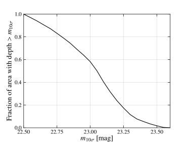
Figure 15: Area as a function of ($10\sigma$ $i$-band) depth for our DES clustering samples. Traditionally clustering analyses select magnitudes $\leq$ to the depth. We have included $\texttt{MAG\_AUTO\_I}<24$ galaxies, beyond the limiting magnitude of any or our area.

The data represented here are a small fraction of the final DES data volume. In future work, we will generate Balrog catalogs covering all the imaging data. Several simple improvements over the analysis presented here are planned, including folding in photometric redshifts into the measurements (see Bonnett et al. 2015, Sánchez et al. 2014 as references describing photometric redshift estimation for DES); using an input catalog with galaxy colors matched to the DECam filters; embedding the simulations into the full stack of single-epoch images instead of directly into the coadds; and adopting input catalogs spanning a larger range of galaxy properties, in order to avoid the intrinsic sample variance of catalogs drawn from the small COSMOS field.

We anticipate that injection simulations similar to Balrog will be useful for a wide variety of measurements beyond clustering. Accurate models of biases and completeness can, we hope, let modern surveys take full advantage of all the available data.

Appendix A Masking

We apply the mask of Crocce et al. (2015) to our data. This mask is made in a five-step process.

1. Coordinate cuts are made to select area in the SV SPT-E region (cf. Section 3.2). The relevant cut for the area over which we have run Balrog is $\delta>-60$. This avoids areas of high stellar density from the LMC.
   

2. As mentioned in Section 3.4, SExtractor detections include a population with large offsets between windowed centroid measurements in different bands. The SV footprint was pixelized at HEALPix resolution $\texttt{NSIDE}=4096$, masking the 4% of the pixels with the highest density of objects with:

   FLUX_ $$\texttt{AUTO\_G}/\texttt{FLUXERR\_AUTO\_G}>5\;\;\texttt{AND}\;\;$$

   $$\lVert\,\,\,\,(\texttt{ALPHAWIN\_J2000\_G},\texttt{DELTAWIN\_J2000\_G})$$

   $$-(\texttt{ALPHAWIN\_J2000\_I},\texttt{DELTAWIN\_J2000\_I})\,\,\,\,\rVert>1\arcsec$$

   About 25% of the large outlier population is within these regions.
   

3. The mask eliminates areas in close proximity to bright stars from the 2MASS catalog (Skrutskie et al., 2006). A circular exclusion region is drawn around each 2MASS star with radius $(-10\,M_{J}+150)$″, where $M_{J}$ is the $J$-band magnitude, setting a maximum radius of 120″ and eliminating all circles with radius $<30$″. The footprint is pixelized at $\texttt{NSIDE}=4096$ resolution, and HEALPixels whose centers fall within 10″ of any exclusion zone are flagged as bad in the mask.
   

4. The mask selects regions with 10$\sigma$ limiting depth of $\texttt{MAG\_AUTO\_I}>22.5$, where the depths are calculated according to procedure presented in Rykoff et al. (in prep.). Briefly, the SExtractor MAGERR_AUTO vs. MAG_AUTO distribution is fit in pixels of HEALPix resolution NSIDE = 1024 to determine the depth on a coarse scale. The random forest algorithm implemented in sklearn is used to find coefficients on this pixelation scale which fit the depth as a function of:

   1. the MANGLE (Swanson et al., 2008) 10$\sigma{}$ limiting magnitude measurements in 2″ apertures available from DESDM,

   2. maps of the survey observing properties (e.g. airmass, PSF size, etc.) compiled by Leistedt et al. (2015) (see also Section 4.2).

   These products are generated at a finer resolution than the MAGERR_AUTO vs. MAG_AUTO curve can be fit: the maps of Leistedt et al. (2015) at NSIDE = 4096, and MANGLE to arbitrary resolution, meaning the survey depth can then be mapped more finely using the coefficients of these quantities.
   

5. The mask selects regions where at least 80% of the area includes detections. Each region is defined on a HEALPix grid of NSIDE = 4096, checking for detections within each of the 64 subpixels of an NSIDE = 32768 pixelized MANGLE mask.

Appendix B Jackknife Errors

Several instances of the work in this paper make use of jackknife error estimates. We generate jackknife regions for our data’s footprint using a $k$-means algorithm, a method to partition $n$ data points into $k$-clusters, assigning each data point into the cluster with the nearest mean; here, the region closest in angular distance. The set of clusters, $\bm{S}=\left\{S_{1},S_{2},...,S_{k}\right\}$, with centers $\bm{\mu}=\left\{\mu_{1},\mu_{2},...,\mu_{k}\right\}$, is generated by minimizing the within-cluster sum of distance squares:

$$\underset{\bm{S}}{\mathrm{arg\,min}}\sum_{i=1}^{k}\sum_{\bm{x}\in S_{i}}\lVert\bm{x}-\bm{\mu}_{i}\rVert^{2}.$$ (8)

Each datum is associated to the region whose center is nearest on the celestial sphere, where a cluster’s set of associated points has been labeled as $\bm{x}$. For approximately uniform data, $k$-means produces cluster sets roughly equal in number of associated points. Figure 16 shows $k$-means classification for our DES galaxies, after applying the cuts described in Section 3.4; galaxies are colored according to which cluster they were assigned.

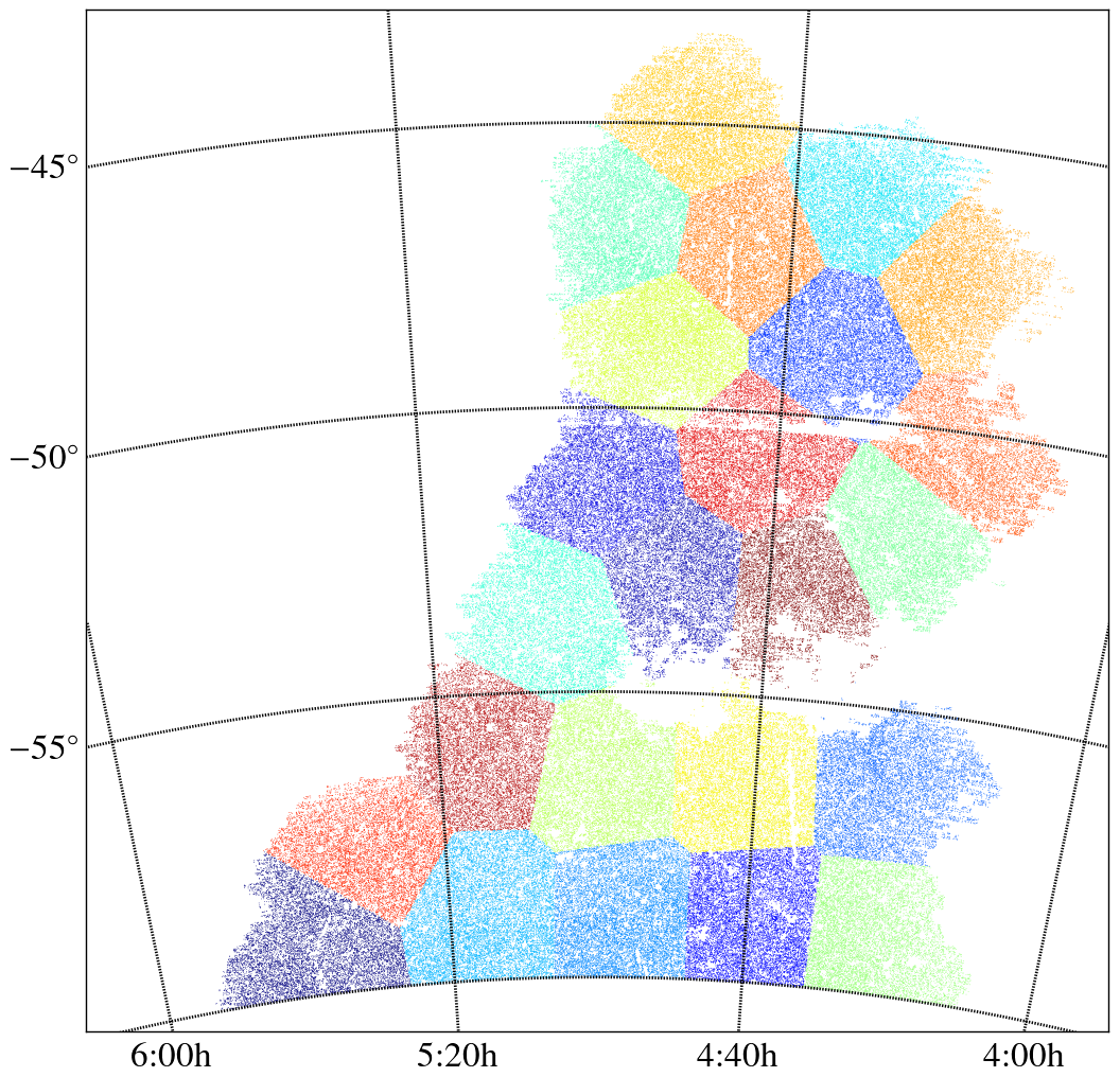
Figure 16: $k$-means jackknife regions. Each point is a DES galaxy, colored according to which of the 24 $k$-means clusters it is assigned membership. The algorithm divides the footprint into regions with roughly uniform cardinality.

After generating $k$-means jackknife regions, we proceed in the usual way to estimate jackknife errors. One $S_{n}$ and its associated $\bm{x}$ is left out in each realization, and we find the covariance of the vector of interest over the realizations:

$$C_{ij}=\frac{(N-1)}{N}\sum_{n=1}^{N}{\left[\vphantom{f_{n}\!\left(x_{j}\right)-f\!\left(x_{j}\right)}f_{n}(x_{i})-f(x_{i})\right]}{\left[f_{n}(x_{j})-f(x_{j})\right]},$$ (9)

where $f$ is the measurement over the full area, without removing any of the sample, and $f_{n}$ is the realization with $S_{n}$ removed. $N$ is the number of jackknife regions; we use $N=24$ throughout this work.

Appendix C Benchmark Comparison

Some of the ongoing and planned clustering analyses of DES data make use of the benchmark sample, which is described in full in Crocce et al. (2015). This sample uses the mask described in Appendix A. Galaxies are selected with a magnitude cut $18<\texttt{MAG\_AUTO\_I}<22.5$. Star-galaxy separation is performed using a new quantity, termed WAVG_SPREAD_MODEL, which is a weighted average of the SExtractor SPREAD_MODEL quantity estimated from stars in the single-epoch DES images. Crocce et al. (2015) measures the angular clustering of this sample, recovering results that are in general agreement with prior measurements.

We present here an additional, approximate validation of the DES benchmark results. Without Balrog galaxies embedded in single-epoch images, we cannot perfectly capture the effects of the star-galaxy separation used in selecting the benchmark sample. However, we measure and adjust for the stellar contamination as in Section 5.5, thus we do not expect any substantial difference in the resulting measurement.

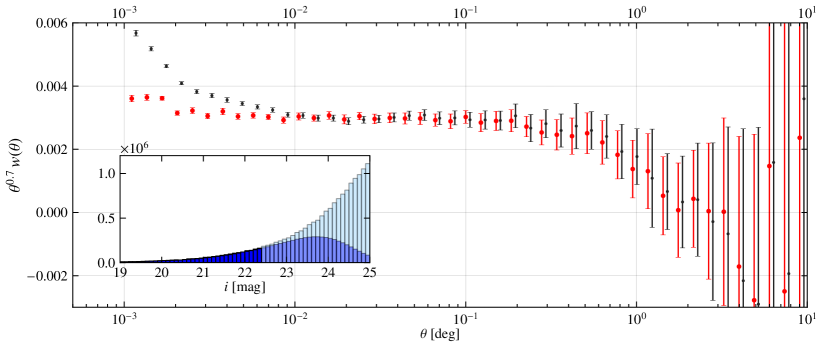
Figure 17: Angular clustering measurements using a sample similar to that of Crocce et al. (2015), with Balrog (red points) and uniform randoms (black points). The figure is similar to Figure 13. Selection cuts are discussed in Section 3.4 and Appendix A. Shown in the inset, a magnitude cut of $18<\texttt{MAG\_AUTO\_I}<22.5$ has been applied; blue is the observed magnitude distribution and light blue is the truth magnitude distribution from Balrog. The correlation functions have been scaled by the approximate power-law slope. The results suggest that the measurements made in Crocce et al. (2015) are unaffected by significant sources of systematic bias at scales $\theta>0.01\degr$.

A comparison between the clustering signals of our benchmark-like sample, measured with uniform and with Balrog randoms, is shown in Figure 17. The results are quantitatively similar to those shown in Figure 13. There is no significant correction introduced by Balrog above $0.01\degr$, suggesting that the benchmark sample is unaffected by significant measurement biases at moderate and large scales. This is consistent with the independent measurements from Crocce et al. (2015).

Author affiliations

1. Department of Physics, The Ohio State University, Columbus, OH 43210, USA

2. Center for Cosmology and Astro-Particle Physics, The Ohio State University, Columbus, OH 43210, USA

3. Institut de Física d’Altes Energies, Universitat Autònoma de Barcelona, E-08193 Bellaterra, Barcelona, Spain

4. Department of Physics & Astronomy, University College London, Gower Street, London, WC1E 6BT, UK

5. Jodrell Bank Center for Astrophysics, School of Physics and Astronomy, University of Manchester, Oxford Road, Manchester, M13 9PL, UK

6. Institut de Ciències de l’Espai, IEEC-CSIC, Campus UAB, Carrer de Can Magrans, s/n, 08193 Bellaterra, Barcelona, Spain

7. Kavli Institute for Particle Astrophysics & Cosmology, P. O. Box 2450, Stanford University, Stanford, CA 94305, USA

8. National Accelerator Laboratory, Menlo Park, CA 94025, USA

9. Brookhaven National Laboratory, Bldg 510, Upton, NY 11973, USA

10. Cerro Tololo Inter-American Observatory, National Optical Astronomy Observatory, Casilla 603, La Serena, Chile

11. Department of Physics and Electronics, Rhodes University, PO Box 94, Grahamstown, 6140, South Africa

12. Fermi National Accelerator Laboratory, P. O. Box 500, Batavia, IL 60510, USA

13. Institute of Astronomy, University of Cambridge, Madingley Road, Cambridge CB3 0HA, UK

14. Kavli Institute for Cosmology, University of Cambridge, Madingley Road, Cambridge CB3 0HA, UK

15. CNRS, UMR 7095, Institut d’Astrophysique de Paris, F-75014, Paris, France

16. Sorbonne Universités, UPMC Univ Paris 06, UMR 7095, Institut d’Astrophysique de Paris, F-75014, Paris, France

17. Laboratório Interinstitucional de e-Astronomia - LIneA, Rua Gal. José Cristino 77, Rio de Janeiro, RJ - 20921-400, Brazil

18. Observatório Nacional, Rua Gal. José Cristino 77, Rio de Janeiro, RJ - 20921-400, Brazil

19. Department of Astronomy, University of Illinois, 1002 W. Green Street, Urbana, IL 61801, USA

20. National Center for Supercomputing Applications, 1205 West Clark St., Urbana, IL 61801, USA

21. Institute of Cosmology & Gravitation, University of Portsmouth, Portsmouth, PO1 3FX, UK

22. George P. and Cynthia Woods Mitchell Institute for Fundamental Physics and Astronomy, and Department of Physics and Astronomy, Texas A&M University, College Station, TX 77843, USA

23. Excellence Cluster Universe, Boltzmannstr. 2, 85748 Garching, Germany

24. Faculty of Physics, Ludwig-Maximilians University, Scheinerstr. 1, 81679 Munich, Germany

25. Universitäts-Sternwarte, Fakultät für Physik, Ludwig-Maximilians Universität München, Scheinerstr. 1, 81679 München, Germany

26. Department of Physics and Astronomy, University of Pennsylvania, Philadelphia, PA 19104, USA

27. Jet Propulsion Laboratory, California Institute of Technology, 4800 Oak Grove Dr., Pasadena, CA 91109, USA

28. Department of Astronomy, University of Michigan, Ann Arbor, MI 48109, USA

29. Department of Physics, University of Michigan, Ann Arbor, MI 48109, USA

30. Kavli Institute for Cosmological Physics, University of Chicago, Chicago, IL 60637, USA

31. Max Planck Institute for Extraterrestrial Physics, Giessenbachstrasse, 85748 Garching, Germany

32. Australian Astronomical Observatory, North Ryde, NSW 2113, Australia

33. Departamento de Física Matemática, Instituto de Física, Universidade de São Paulo, CP 66318, CEP 05314-970, São Paulo, SP, Brazil

34. Institució Catalana de Recerca i Estudis Avançats, E-08010 Barcelona, Spain

35. Centro de Investigaciones Energéticas, Medioambientales y Tecnológicas (CIEMAT), Madrid, Spain

36. Department of Physics, University of Illinois, 1110 W. Green St., Urbana, IL 61801, USA

37. Argonne National Laboratory, 9700 South Cass Avenue, Lemont, IL 60439, USA

38. Department of Physics, Stanford University, 382 Via Pueblo Mall, Stanford, CA 94305, USA

References

- Bergé et al. (2013) Bergé J., Gamper L., Réfrégier A., Amara A., 2013, Astronomy and Computing, 1, 23
- Bertin (2006) Bertin E., 2006, in Gabriel C., Arviset C., Ponz D., Enrique S., eds, Astronomical Society of the Pacific Conference Series Vol. 351, p. 112
- Bertin (2011) Bertin E., 2011, in Evans I. N., Accomazzi A., Mink D. J., Rots A. H., eds, Astronomical Society of the Pacific Conference Series Vol. 442, p. 435
- Bertin & Arnouts (1996) Bertin E., Arnouts S., 1996, A&AS, 117, 393
- Bertin et al. (2002) Bertin E., Mellier Y., Radovich M., Missonnier G., Didelon P., Morin B., 2002, in Bohlender D. A., Durand D., Handley T. H., eds, Astronomical Society of the Pacific Conference Series Vol. 281, p. 228
- Blake et al. (2010) Blake C. et al., 2010, MNRAS, 406, 803
- Bonnett et al. (2015) Bonnett C. et al., 2015, arXiv:1507.05909
- Bouy et al. (2013) Bouy H., Bertin E., Moraux E., Cuillandre J.-C., Bouvier J., Barrado D., Solano E., Bayo A., 2013, A&A, 554, A101
- Busha et al. (2013) Busha M. T., Wechsler R. H., Becker M. R., Erickson B., Evrard A. E., 2013, in American Astronomical Society Meeting Abstracts 221, p. 341.07
- Capak et al. (2007) Capak P. et al., 2007, ApJS, 172, 99
- Chang et al. (2015) Chang C. et al., 2015, ApJ, 801, 73
- Crocce et al. (2011) Crocce M., Gaztañaga E., Cabré A., Carnero A., Sánchez E., 2011, MNRAS, 417, 2577
- Crocce et al. (2015) Crocce M. et al., 2015, arXiv:1507.05360
- Dark Energy Survey Collaboration (2005) Dark Energy Survey Collaboration 2005, ArXiv Astrophysics e-prints
- Desai et al. (2012) Desai S. et al., 2012, ApJ, 757, 83
- Diehl et al. (2014) Diehl H. T. et al., 2014, in Society of Photo-Optical Instrumentation Engineers (SPIE) Conference Series, p. 0
- Dressler et al. (2012) Dressler A. et al., 2012, arXiv:1210.7809
- Eisenstein et al. (2001) Eisenstein D. J. et al., 2001, AJ, 122, 2267
- Flaugher et al. (2015) Flaugher B. et al., 2015, arXiv:1504.02900
- Foreman-Mackey et al. (2013) Foreman-Mackey D., Hogg D. W., Lang D., Goodman J., 2013, PASP, 125, 306
- Greisen & Calabretta (2002) Greisen E. W., Calabretta M. R., 2002, A&A, 395, 1061
- Górski et al. (2005) Górski K. M., Hivon E., Banday A. J., Wandelt B. D., Hansen F. K., Reinecke M., Bartelmann M., 2005, ApJ, 622, 759
- Hanisch et al. (2001) Hanisch R. J., Farris A., Greisen E. W., Pence W. D., Schlesinger B. M., Teuben P. J., Thompson R. W., Warnock III A., 2001, A&A, 376, 359
- High et al. (2009) High F. W., Stubbs C. W., Rest A., Stalder B., Challis P., 2009, AJ, 138, 110
- Ilbert et al. (2006) Ilbert O. et al., 2006, A&A, 457, 841
- Ilbert et al. (2009) Ilbert O. et al., 2009, ApJ, 690, 1236
- Jarvis et al. (2004) Jarvis M., Bernstein G., Jain B., 2004, MNRAS, 352, 338
- Jouvel et al. (2009) Jouvel S. et al., 2009, A&A, 504, 359
- Kelly et al. (2014) Kelly P. L. et al., 2014, MNRAS, 439, 28
- Landy & Szalay (1993) Landy S. D., Szalay A. S., 1993, ApJ, 412, 64
- Laureijs et al. (2012) Laureijs R. et al., 2012, in Society of Photo-Optical Instrumentation Engineers (SPIE) Conference Series, p. 0
- Leauthaud et al. (2007) Leauthaud A. et al., 2007, ApJS, 172, 219
- Lee et al. (1962) Lee S., Ditko S., Kirby, J. 1962, in Amazing Fantasy #15
- Leistedt et al. (2015) Leistedt B. et al., 2015, arXiv:1507.05647
- Lewis et al. (2000) Lewis A., Challinor A., Lasenby A., 2000, ApJ, 538, 473
- Lima et al. (2008) Lima M., Cunha C. E., Oyaizu H., Frieman J., Lin H., Sheldon E. S., 2008, MNRAS, 390, 118
- Maddox et al. (1996) Maddox S. J., Efstathiou G., Sutherland W. J., 1996, MNRAS, 283, 1227
- Mandelbaum et al. (2014) Mandelbaum R. et al., 2014, ApJS, 212, 5
- Manfroid (1995) Manfroid J., 1995, A&AS, 113, 587
- McCracken et al. (2007) McCracken H. J. et al., 2007, ApJS, 172, 314
- Miyazaki et al. (2002) Miyazaki S. et al., 2002, PASJ, 54, 833
- Mohr et al. (2012) Mohr J. J. et al., 2012, in Society of Photo-Optical Instrumentation Engineers (SPIE) Conference Series, p. 0
- Myers et al. (2006) Myers A. D. et al., 2006, ApJ, 638, 622
- Nock et al. (2010) Nock K., Percival W. J., Ross A. J., 2010, MNRAS, 407, 520
- Padmanabhan et al. (2007) Padmanabhan N. et al., 2007, MNRAS, 378, 852
- Perlmutter et al. (1999) Perlmutter S. et al., 1999, ApJ, 517, 565
- Riess et al. (1998) Riess A. G. et al., 1998, AJ, 116, 1009
- Ross et al. (2011a) Ross A. J., Percival W. J., Crocce M., Cabré A., Gaztañaga E., 2011a, MNRAS, 415, 2193
- Ross et al. (2011b) Ross A. J. et al., 2011b, MNRAS, 417, 1350
- Ross et al. (2012) Ross A. J. et al., 2012, MNRAS, 424, 564
- Rowe et al. (2014) Rowe B. et al., 2014, arXiv:1407.7676
- Ruhl et al. (2004) Ruhl J. et al., 2004, in Bradford C. M. et al., eds, Society of Photo-Optical Instrumentation Engineers (SPIE) Conference Series Vol. 5498, pp 11–29
- Schlafly et al. (2012) Schlafly E. F. et al., 2012, ApJ, 756, 158
- Schlegel et al. (2009) Schlegel D., White M., Eisenstein D., 2009, in astro2010: The Astronomy and Astrophysics Decadal Survey, p. 314
- Schneider et al. (2002) Schneider P., van Waerbeke L., Kilbinger M., Mellier Y., 2002, A&A, 396, 1
- Scranton et al. (2002) Scranton R. et al., 2002, ApJ, 579, 48
- Skrutskie et al. (2006) Skrutskie M. F. et al., 2006, AJ, 131, 1163
- Soumagnac et al. (2015) Soumagnac M. T. et al., 2015, MNRAS, 450, 666
- Swanson et al. (2008) Swanson M. E. C., Tegmark M., Hamilton A. J. S., Hill J. C., 2008, MNRAS, 387, 1391
- Sánchez et al. (2014) Sánchez C. et al., 2014, MNRAS, 445, 1482
- Tucker et al. (2007) Tucker D. L. et al., 2007, in Sterken C., ed., Astronomical Society of the Pacific Conference Series Vol. 364, p. 187
- Vikram et al. (2015) Vikram V. et al., 2015, arXiv:1504.03002
- Weinberg et al. (2013) Weinberg D. H., Mortonson M. J., Eisenstein D. J., Hirata C., Riess A. G., Rozo E., 2013, Phys. Rep., 530, 87
- York et al. (2000) York D. G. et al., 2000, AJ, 120, 1579
- Zacharias et al. (2013) Zacharias N., Finch C. T., Girard T. M., Henden A., Bartlett J. L., Monet D. G., Zacharias M. I., 2013, AJ, 145, 44
- Zwicky (1937) Zwicky F., 1937, ApJ, 86, 217