A risk analysis for a system stabilized by a central agent

Abstract.

We formulate and analyze a multi-agent model for the evolution of individual and systemic risk in which the local agents interact with each other through a central agent who, in turn, is influenced by the mean field of the local agents. The central agent is stabilized by a bistable potential, the only stabilizing force in the system. The local agents derive their stability only from the central agent. In the mean field limit of a large number of local agents we show that the systemic risk decreases when the strength of the interaction of the local agents with the central agent increases. This means that the probability of transition from one of the two stable quasi-equilibria to the other one decreases. We also show that the systemic risk increases when the strength of the interaction of the central agent with the mean field of the local agents increases. Following the financial interpretation of such models and their behavior given in our previous paper (Garnier, Papanicolaou and Yang, SIAM J. Fin. Math. 4, 2013, 151-184), we may interpret the results of this paper in the following way. From the point of view of systemic risk, and while keeping the perceived risk of the local agents approximately constant, it is better to strengthen the interaction of the local agents with the central agent than the other way around.

1. Introduction

In recent years, interacting particle systems have been extensively used to model financial systemic risk for complex, inter-connected systems. An interacting particle system with binary risk variables is considered in [4] and the law of large numbers, central limit theorem and large deviation principle are derived for this model. An interacting particle system of diffusion processes is used in [9] to model the interbank lending system. In [3], a model simplified from the one in [9] is considered, in which each agent can control the lending flow rate and optimizes the individual objective function, and thus the system can be put in the framework of mean field games. In [15], the authors use interacting Bessel-like diffusion processes to model systemic risk and establish a large deviation principle. In [10, 11], we consider an interacting particle system with a bistable potential and we use the large deviation principle to explain that the overall systemic risk may increase while individual risks are decreased. The large deviation principle in [10, 11] is solved numerically in [17]. In [1], the authors consider interacting jump-diffusion processes modeling interbank lending and borrowing and prove the weak law of large numbers (LLN) of the empirical measure as the number of individuals goes to infinity, and define systemic indicators based on the LLN result. In [13, 20, 14, 21], the authors model large portfolios and default clustering and derive the law of large numbers, fluctuation analysis and large deviations.

In our previous work [10], we used an interacting agent-based, mean-field model to show that individual risk may not affect systemic risk in an obvious way. That is, each agent may have relatively low individual risk by diversification through risk-sharing while the overall, systemic risk is increased as a result of diversification. We considered the following model that was studied extensively before by [5, 6, 12, 7]:

(1) $$dx_{j}(t)=-hV^{\prime}(x_{j}(t))dt-\theta(x_{j}(t)-\bar{x}_{N}(t))dt+\sigma dW^{j}_{t},\quad\quad j=1,\ldots,N,$$

where $x_{j}(t)$ represents a risk variable for agent $j$ at time $t$ and $N$ is the number of agents. The potential $V(x)=\frac{1}{4}x^{4}-\frac{1}{2}x^{2}$ is taken to be bistable with two stable states $\pm 1$, and the constant $h>0$ quantifies intrinsic stability for each agent. We define $-1$ as the normal state of an agent and $+1$ as the failed state. The empirical mean $\bar{x}_{N}(t):=\frac{1}{N}\sum_{j=1}^{N}x_{j}(t)$ is the mean risk, and the constant $\theta$ is positive so that $x_{j}$ tends to stay close to $\bar{x}_{N}$. The standard Brownian motions $\{W^{j}_{t}\}_{j=1}^{N}$ are independent and model external risk factors, with $\sigma>0$ their strength.

It was shown in [5] that the empirical measure $U_{N}(t,dx):=\frac{1}{N}\sum_{j=1}^{N}\delta_{x_{j}(t)}(dx)$ converges weakly in probability to $u(t,dx)=u(t,x)dx$, the weak solution of the nonlinear Fokker-Planck equation:

$$\frac{\partial}{\partial t}u=h\frac{\partial}{\partial x}\left[V^{\prime}(x)u\right]-\theta\frac{\partial}{\partial x}\left\{\left[\int_{-\infty}^{\infty}yu(t,dy)-x\right]u\right\}+\frac{1}{2}\sigma^{2}\frac{\partial^{2}}{\partial x^{2}}u,$$

starting from $u(0,dx)=\lim_{N\to\infty}U_{N}(0,dx)$ (provided the weak limit exists). Given $h$ and $\theta$, for sufficiently small $\sigma$, $u(t,x)$ has two equilibria $u^{e}_{\pm\xi_{b}}(x):=\lim_{t\to\infty}u(t,x)$, where $\bar{x}_{N}(t)$ converges to either $\xi_{b}>0$ or $-\xi_{b}$ as $t\to\infty$, depending on the initial condition. Thus we define $u^{e}_{-\xi_{b}}$ as the normal state of the system and $u^{e}_{+\xi_{b}}$ as the failed state of the system.

Given that $N$ is large but finite, and $U_{N}(0,dx)\approx u^{e}_{-\xi_{b}}(x)dx$, we showed [10, Theorem 6.2 and Corollary 6.4] that by using the large deviation principle in [6] and assuming that $h$ is small, the systemic risk, defined as the probability of the transition of $U_{N}(t,dx)$ from $u^{e}_{-\xi_{b}}(x)dx$ at time $0$ to $u^{e}_{+\xi_{b}}(x)dx$ at some time $t\leq T<\infty$ has the following exponentially small but nonzero value:

(2) $$\mathbb{P}\left(U_{N}(0,dx)\approx u^{e}_{-\xi_{b}}(x)dx,~{}U_{N}(t,dx)\approx u^{e}_{+\xi_{b}}(x)dx~{}~{}t\leq T<\infty\right)\overset{\begin{subarray}{c}N\gg 1\\ h\ll 1\end{subarray}}{\approx}\exp\left(-N\frac{2\xi_{b}^{2}}{\sigma^{2}T}\right),$$

where

$$\xi_{b}=\sqrt{1-3\frac{\sigma^{2}}{2\theta}}\left(1+h\frac{6}{\sigma^{2}}\left(\frac{\sigma^{2}}{2\theta}\right)^{2}\frac{1-2(\sigma^{2}/2\theta)}{1-3(\sigma^{2}/2\theta)}\right)+O(h^{2}).$$

Fluctuation analysis on (1) [10, Lemma 6.5], shows that the risk of each agent has the form $x_{j}(t)=-1+z_{j}(t)$ and $\lim_{t\to\infty}\mathbf{Var}z_{j}(t)\lesssim\frac{\sigma^{2}}{2\theta}$. Thus, the quantity $\frac{\sigma^{2}}{2\theta}$ can be considered as the individual risk for each agent.

We then see that if the strength of the external risk $\sigma^{2}$ is increased, either because the agents are more risk-prone or because the economic environment is more uncertain, then the agents can increase $\theta$, the risk-diversification parameter, so that that their individual risk is still low. However, from the analysis of the systemic risk (2) we see that the systemic risk is increased when $\sigma^{2}$ increases even if the individual risk ${\sigma^{2}}/({2\theta})$ is very low: there is a systemic level effect of $\sigma^{2}$ that cannot be observed by the agents and it tends to destabilize the system.

In this paper, we extend the previous model (1) by introducing a central agent with the risk variable $x_{0}^{(N)}(t)$. The model we study in this paper is given by

(3) $$dx_{0}^{(N)}=-h_{0}V_{0}^{\prime}(x_{0}^{(N)})dt-\theta_{0}(x_{0}^{(N)}-\bar{x}_{N})dt+\frac{\sigma_{0}}{\sqrt{N}}dW^{0}_{t},\quad\quad\bar{x}_{N}=\frac{1}{N}\sum_{j=1}^{N}x_{j},$$

(4) $$dx_{j}=-hV^{\prime}(x_{j})dt-\theta\big{(}x_{j}-x_{0}^{(N)}\big{)}dt+\sigma dW^{j}_{t},\quad\quad j=1,\ldots,N.$$

Here $V_{0}(x)$ and $V(x)$ are potentials with two stable states and in this paper we again assume that $V_{0}(x)=V(x)=\frac{1}{4}x^{4}-\frac{1}{2}x^{2}$ with the stable states $\pm 1$. The parameters $h_{0},h\geq 0$ are the strengths of intrinsic stability of the central and local agents, respectively. The parameters $\theta_{0},\theta\geq 0$ determine the strength of the mean-field interactions. The central agent $x_{0}^{(N)}$ is intrinsically stable when $h_{0}>0$ and may be destabilized through a mean field interaction with the local agents where $\theta_{0}>0$. Depending on whether $h>0$ or $h=0$, the local agents $\{x_{j}\}_{j=1}^{N}$ are or are not intrinsically stable. They may be stabilized through their interaction with the central agent $x_{0}^{(N)}$. The independent, standard Brownian motions $\{W_{t}^{j}\}_{j=0}^{N}$ model the external risk for the central and local agents. We note that the normalization factor $1/\sqrt{N}$ in (3) makes $x_{0}^{(N)}$ and $\bar{x}_{N}$ have external risks of comparable size for $N$ large, and we will assume that $\sigma_{0}<\sigma$ or $\sigma_{0}=0$ since we want the central agent to operate with less risk than the local agents.

In the regime of no cooperation, $\theta_{0}=\theta=0$, the central agent and the local agents are independent of each other and Kramers’ large deviation law states that when $\sigma_{0}$ and $\sigma$ are small, the probabilities of transition from one stable state to the other within the time interval $[0,T]$ are proportional to $T\exp(-2h_{0}V_{0}(0)/\sigma_{0}^{2})$ and $T\exp(-2hV(0)/\sigma^{2})$, for the central and local agents, respectively. We want to analyze stabilization effects in the cooperative regime $\theta_{0},\theta>0$.

In this paper, we will assume that the intrinsic stability of the local agents, $h$, is exactly zero, while we only assume that $h$ is small in [10]. Because of this simplifying assumption, instead of considering the pair $(x_{0}^{(N)}(t),\frac{1}{N}\sum_{j=1}^{N}\delta_{x_{j}(t)}(dx))$ as a scalar and a measure-valued process, we can simply consider $(x_{0}^{(N)}(t),\bar{x}_{N}(t))$ as a two-dimensional process and get results that are more detailed than it was possible in the setup of [10]. First, we compute numerically the minimizing path for the associated large deviation problem, and we are able to explore how the various parameters affect the agents’ fluctuations and the systemic risk. We also recover the main result in [10], that is, that the systemic risk is increased, with the local risks kept fixed, if we increase $\sigma^{2}$ and $\theta$ with the ratio $\sigma^{2}/\theta$ fixed. Another result is that because we assume that $0=h<h_{0}$ and $\sigma_{0}<\sigma$, the central agent is more stable than the empirical mean of the local agents. In this setting, we find that $\theta_{0}$ and $\theta$ tend to play opposite roles: higher $\theta_{0}$ increases the systemic risk as we force the stable term $x_{0}^{(N)}$ to be close to the relatively unstable term $\bar{x}$, but on the other hand, increasing $\theta$ lowers the systemic risk as $\bar{x}$ tends to be close to $x_{0}^{(N)}$. This is the main result of this paper. The third result here, for a case not considered in the previous paper, concerns the introduction of optimal controls for the local agents. We use optimal control theory and find that the use of controls amounts to replacing $\theta$ by an effective one that is larger, and thus it reduces the systemic risk.

This paper is organized as follows. In Section 2 we state the mean field limit of the pair $(x_{0}^{(N)}(t),\frac{1}{N}\sum_{j=1}^{N}\delta_{x_{j}(t)}(dx))$ as $N\to\infty$. We then discuss the equilibria of the limit Fokker-Planck equation. In Section 3 we analyze the special case where $h$ is exactly zero. In this case, explicit solutions of the fluctuation analysis can be obtained, and we have a large deviations principle for $(x_{0}^{(N)}(t),\bar{x}_{N}(t))$ using the Freidlin-Wentzell theory. In Section 4 we give the formal large deviation principle for the empirical measure $(x_{0}^{(N)}(t),\frac{1}{N}\sum_{j=1}^{N}\delta_{x_{j}(t)}(dx))$ that is necessary when $h>0$. We do not use this general formulation but we do show that the large deviation problems for $(x_{0}^{(N)}(t),\bar{x}_{N}(t))$ and $(x_{0}^{(N)}(t),\frac{1}{N}\sum_{j=1}^{N}\delta_{x_{j}(t)}(dx))$ are the same if $h=0$. In Section 5 we formulate a control problem for the local agents in (4) and use optimal control theory to analyze the effect of the control on the system. Finally, in Section 6 we present results of extensive numerical simulations. The technical details of the proofs are in the appendices.

2. The mean field limit of a large number of local agents

We begin by recalling the main results of mean field limit theory as they apply to problem (3),(4), in the next section, and then discuss the equilibrium solutions of the limit, non-linear Fokker-Planck equation.

2.1. The non-linear Fokker-Planck equation

The stochastic model (3),(4) is a simple extension of the model in [5, 12] (see also [23, 22, 18, 16]). We let $M_{1}(\mathbb{R})$ denote the space of probability measures endowed with the metric of the weak convergence, and $C([0,T],M_{1}(\mathbb{R}))$ the space of continuous $M_{1}(\mathbb{R})$-valued processes in the time interval $[0,T]$ endowed with the maximum distance in $[0,T]$. In the limit $N\to\infty$, the pair $(x_{0}^{(N)}(t),\frac{1}{N}\sum_{j=1}^{N}\delta_{x_{j}(t)}(dx))$ converges in $(\mathbb{R},M_{1}(\mathbb{R}))$ to $(y_{0}(t),p(t,x)dx)$ in probability, the weak solution of the nonlinear Fokker-Planck equation and ordinary differential equation

(5) $$\frac{d}{dt}y_{0}=-h_{0}V_{0}^{\prime}(y_{0})-\theta_{0}\Big{(}y_{0}-\int xp(t,x)dx\Big{)},$$

(6) $$\frac{\partial}{\partial t}p(t,x)=h\frac{\partial}{\partial x}[V^{\prime}(x)p(t,x)]+\theta\frac{\partial}{\partial x}[(x-y_{0}(t))p(t,x)]+\frac{\sigma^{2}}{2}\frac{\partial^{2}}{\partial x^{2}}p(t,x),$$

with the initial condition $y_{0}(0)=\lim_{N\to\infty}x_{0}^{(N)}(0)$ and $p(0,dx)=\lim_{N\to\infty}\frac{1}{N}\sum_{j=1}^{N}\delta_{x_{j}(0)}(dx)$, given that the limits exist. Equivalently, we can characterize the pair $(y_{0}(t),p(t,x)dx)$ by noting that $p(t,x)$ is the transition probability density of the process $X_{t}$, the solution of

$$\frac{d}{dt}y_{0}=-h_{0}V_{0}^{\prime}(y_{0})-\theta_{0}(y_{0}-\mathbb{E}X_{t}),$$

$$dX_{t}=-hV^{\prime}(X_{t})dt-\theta(X_{t}-y_{0})dt+\sigma dW_{t},$$

where $W_{t}$ is a standard Brownian motion. In addition, if $h=0$ and $\bar{y}(t):=\mathbb{E}(X_{t})$, then $(y_{0}(t),\bar{y}(t))$ satisfies

(7) $$\frac{d}{dt}y_{0}=-h_{0}V_{0}^{\prime}(y_{0})-\theta_{0}(y_{0}-\bar{y}),$$

(8) $$\frac{d}{dt}\bar{y}=-\theta(\bar{y}-y_{0}).$$

2.2. Equilibrium states

Given the existence of a stationary state $(y_{0}^{e},p^{e}(x;y_{0}^{e})):=(\lim_{t\to\infty}y_{0}(t),\lim_{t\to\infty}p(t,x))$, it satisfies

(9) $$p^{e}(x;y_{0}^{e})=\frac{1}{Z(y_{0}^{e})}\exp\Big{(}-\frac{2hV(x)+\theta(x-y_{0}^{e})^{2}}{\sigma^{2}}\Big{)},$$

which is obtained from (6), and satisfies the consistency equation

(10) $$\int xp^{e}(x;y_{0}^{e})dx=y_{0}^{e}+\frac{h_{0}}{\theta_{0}}V_{0}^{\prime}(y_{0}^{e}),$$

obtained from (5). If $h=0$, then $p^{e}(x;y_{0}^{e})$ is a Gaussian density function, given by (9), with mean $y_{0}^{e}$ and (10) implies $V_{0}^{\prime}(y_{0}^{e})=0$. Therefore $y_{0}^{e}=\pm 1$. The equilibrium states for the system are determined by the equilibrium states of the central agent. Indeed, if the central agent takes the equilibrium value $y_{0}^{e}=-1$, then the individual agents take a Gaussian distribution with mean $-1$ and variance $\sigma^{2}/(2\theta)$:

(11) $$p^{e}(x)=\frac{1}{\sqrt{\pi\frac{\sigma^{2}}{\theta}}}\exp\Big{(}-\frac{\theta(x+1)^{2}}{\sigma^{2}}\Big{)}.$$

When $h$ is positive but small, we let $y_{0}^{e0}=\pm 1$ and therefore $V_{0}^{\prime}(y_{0}^{e0})=0$ with $V_{0}^{\prime\prime}(y_{0}^{e0})>0$. It is then possible to find an equilibrium state $y_{0}^{e-}$, resp. $y_{0}^{e+}$, close to $y_{0}^{e0}=-1$, resp. $y_{0}^{e0}=1$, and we have

$$y_{0}^{e}=y_{0}^{e0}+hy_{0}^{e1}+o(h),$$

with

$$y_{0}^{e1}=-\frac{\theta_{0}}{h_{0}\theta V_{0}^{\prime\prime}(y_{0}^{e1})}\frac{\int e^{-\theta x^{2}/\sigma^{2}}V^{\prime}(y_{0}^{e0}+x)dx}{\int e^{-\theta x^{2}/\sigma^{2}}dx}.$$

If $V_{0}(x)=V(x)=\frac{1}{4}x^{4}-\frac{1}{2}x^{2}$ then $y_{0}^{e0}=\pm 1$ and $y_{0}^{e1}=\mp\frac{3\theta_{0}\sigma^{2}}{4h_{0}\theta^{2}}$. This result shows that the positions of the equilibrium states of the central agent will be shifted when the individual agents have their own stabilization potential. The states $y_{0}^{e-}$ and $y_{0}^{e+}$ are the two equilibrium states of the central agent, and $y_{0}^{e-}+(h_{0}/\theta_{0})V_{0}^{\prime}(y_{0}^{e-})$ and $y_{0}^{e+}+(h_{0}/\theta_{0})V_{0}^{\prime}(y_{0}^{e+})$ are the two associated equilibrium means of the individual agents.

3. The case of no intrinsic stabilization for the local agents ($h=0$)

In this section we consider the special case where the individual agents have no intrinsic stability, i.e., $h=0$. In this case, (4) is linear so instead of considering the empirical distribution $\frac{1}{N}\sum_{j=1}^{N}\delta_{x_{j}(t)}(dx)$, we can focus on the empirical mean $\bar{x}_{N}(t)=\frac{1}{N}\sum_{j=1}^{N}x_{j}(t)$. The pair $(x_{0}^{(N)}(t),\bar{x}_{N}(t))$ satisfies the joint SDEs:

(12) $$dx_{0}^{(N)}=-h_{0}V_{0}^{\prime}(x_{0}^{(N)})dt-\theta_{0}(x_{0}^{(N)}-\bar{x}_{N})dt+\frac{\sigma_{0}}{\sqrt{N}}dW^{0}_{t},$$

$$d\bar{x}_{N}=-\theta(\bar{x}_{N}-x_{0}^{(N)})dt+\frac{\sigma}{\sqrt{N}}d\bar{W}_{t}^{(N)},$$

where $\bar{W}_{t}^{(N)}=\frac{1}{\sqrt{N}}\sum_{j=1}^{N}W^{j}_{t}$ is a standard Brownian motion independent of $W^{0}_{t}$. The mean-field limit, $(y_{0}(t),\bar{y}(t)):=\lim_{N\to\infty}(x_{0}^{(N)}(t),\bar{x}_{N}(t))$, satisfies (7) with the equilibria $y_{0}^{e}:=\lim_{t\to\infty}y_{0}(t)=\pm 1$ and $\bar{y}^{e}:=\lim_{t\to\infty}\bar{y}(t)=\pm 1$ depending on the initial condition $(y_{0}(0),\bar{y}(0))$.

3.1. Fluctuation analysis in the case $h=0$

Here we analyse the fluctuations of $(x_{0}^{(N)}(t),\bar{x}_{N}(t))$ centred at $(y_{0}(t),\bar{y}(t))$ when $N$ is large. To simplify, we assume that $y_{0}(0)=y_{0}^{e}=-1$ and $\bar{y}(0)=\bar{y}^{e}=-1$, and thus $y_{0}(t)\equiv y_{0}^{e}=-1$ and $\bar{y}(0)\equiv\bar{y}^{e}=-1$. Define $z_{0}^{(N)}=\sqrt{N}(x_{0}^{(N)}-y_{0}^{e})$ and $\bar{z}_{N}=\sqrt{N}(\bar{x}_{N}-\bar{y}^{e})$. As $N\to\infty$, $(z_{0}^{(N)},\bar{z}_{N})$ converges in distribution to the process $(z_{0},\bar{z})$ where

(13) $$dz_{0}=-h_{0}V_{0}^{\prime\prime}(y_{0}^{e})z_{0}dt-\theta_{0}(z_{0}-\bar{z})dt+\sigma_{0}dW^{0}_{t},$$

$$d\bar{z}=-\theta(\bar{z}-z_{0})dt+\sigma d\bar{W}_{t},$$

where $\bar{W}_{t}$ is a standard Brownian motion independent of $W^{0}_{t}$. This means that, when $N$ is large, $x_{0}^{(N)}(t)\approx y_{0}^{e}+\frac{1}{\sqrt{N}}z_{0}$ and $\bar{x}(t)\approx\bar{y}^{e}+\frac{1}{\sqrt{N}}\bar{z}$ in distribution. Because $y_{0}^{e}=\bar{y}^{e}=-1$ is the normal state, $z_{0}$ and $\bar{z}$ are regarded as the central risks (as opposed to the large deviations that will be discussed in the next section) of $x_{0}^{(N)}$ and $\bar{x}_{N}$, respectively. We note that (13) is a system of linear differential equations and thus the explicit solution is:

$$\begin{pmatrix}z_{0}(t)\\ \bar{z}(t)\end{pmatrix}=e^{t{\bf A}}\begin{pmatrix}z_{0}(0)\\ \bar{z}(0)\end{pmatrix}+\int_{0}^{t}e^{(t-s){\bf A}}\begin{pmatrix}\sigma_{0}dW^{0}_{s}\\ \sigma d\bar{W}_{s}\end{pmatrix},\quad{\bf A}=\begin{pmatrix}-h_{0}V_{0}^{\prime\prime}(y_{0}^{e})-\theta_{0}&\theta_{0}\\ \theta&-\theta\end{pmatrix}.$$

Therefore $(z_{0}(t),\bar{z}(t))$ is a Gaussian process with

(14) $$\mathbb{E}\begin{pmatrix}z_{0}(t)\\ \bar{z}(t)\end{pmatrix}=e^{t{\bf A}}\begin{pmatrix}z_{0}(0)\\ \bar{z}(0)\end{pmatrix},$$

(15) $$\begin{pmatrix}\mathbf{Var}z_{0}(t)&\mathbf{Cov}(z_{0}(t),\bar{z}(t))\\ \mathbf{Cov}(z_{0}(t),\bar{z}(t))&\mathbf{Var}\bar{z}(t)\end{pmatrix}=\int_{0}^{t}e^{(t-s){\bf A}}\begin{pmatrix}\sigma_{0}^{2}&0\\ 0&\sigma^{2}\end{pmatrix}e^{(t-s){\bf A}^{\mathbf{T}}}ds.$$

We want to analyse the impact of the various parameters on $(z_{0}(t),\bar{z}(t))$, in particular, for the case that $t\to\infty$ and $\sigma,\theta\to\infty$ with a fixed ratio $\alpha:=\sigma^{2}/\theta<\infty$. To do this, we use the eigen-decomposition of ${\bf A}$ to compute (15) and obtain the following.

Proposition 1.

If $h_{0}$, $\theta_{0}$ and $\theta$ are positive, then $\lim_{t\to\infty}\mathbb{E}z_{0}(t)=\lim_{t\to\infty}\mathbb{E}\bar{z}(t)=0$. In addition, the variances and covariance of the fluctuations $z_{0}(t)$ and $\bar{z}(t)$ have the following limits as $t\to\infty$ and $\sigma,\theta\to\infty$ with a fixed ratio $\alpha=\sigma^{2}/\theta<\infty$:

(16) $$\lim_{\begin{subarray}{c}\sigma,\theta\to\infty\\ \sigma^{2}/\theta=\alpha\end{subarray}}\lim_{t\to\infty}\mathbf{Var}z_{0}(t)=\frac{\sigma_{0}^{2}}{2h_{0}V_{0}^{\prime\prime}(y_{0}^{e})},$$

(17) $$\lim_{\begin{subarray}{c}\sigma,\theta\to\infty\\ \sigma^{2}/\theta=\alpha\end{subarray}}\lim_{t\to\infty}\mathbf{Var}\bar{z}(t)=\frac{\sigma_{0}^{2}}{2h_{0}V_{0}^{\prime\prime}(y_{0}^{e})}+\frac{\sigma^{2}}{2\theta},$$

(18) $$\lim_{\begin{subarray}{c}\sigma,\theta\to\infty\\ \sigma^{2}/\theta=\alpha\end{subarray}}\lim_{t\to\infty}\mathbf{Cov}(z_{0}(t),\bar{z}(t))=\frac{\sigma_{0}^{2}}{2h_{0}V_{0}^{\prime\prime}(y_{0}^{e})}.$$

This means that after the limits are applied, $z_{0}=Z_{1}$ and $\bar{z}=Z_{1}+Z_{2}$, where $Z_{1}$ and $Z_{2}$ are two independent Gaussian random variables with mean $0$ and variances $\frac{\sigma_{0}^{2}}{2h_{0}V_{0}^{\prime\prime}(y_{0}^{e})}$ and $\frac{\sigma^{2}}{2\theta}$, respectively.

Proof.

This involves basic computations given in Appendix A.1. ∎

We see that the variances and the covariance of the limits of $z_{0}$ and $\bar{z}$ increase with increasing $\sigma_{0}$ or decreasing $h_{0}$. We also note that these three statistics blow up as $\sigma_{0}\to\infty$ even if $\sigma_{0}^{2}/\theta_{0}$ is finite and small. This is because when $h$ is exactly zero, $\bar{x}_{N}$ cannot serve as a stabilizing term and $x_{0}^{(N)}$ cannot diversify its risk to $\bar{x}_{N}$ by increasing $\theta_{0}$.

3.2. Large deviations

3.2.1. A general large deviation principle

From the mean field and fluctuation analysis we see that if $N$ is large and $x_{0}^{(N)}(0)=x_{j}(0)=-1$ for all $j=1,\ldots,N$, then one can expect that $(x_{0}^{(N)}(t),\bar{x}_{N}(t))\approx(y_{0}^{e},\bar{y}^{e})=(-1,-1)$ for all $t$. However, as long as $N$ is finite, $x_{0}^{(N)}(t)$ and $\bar{x}_{N}(t)$ are stochastic processes and therefore the event that the overall system has a transition in a finite time interval has a small but nonzero probability. Mathematically speaking, we consider the event of the continuous paths $(x_{0}^{(N)}(t),\bar{x}_{N}(t))\in C([0,T],\mathbb{R}^{2})$ starting from $(y_{0}^{e-},\bar{y}^{e-}):=(-1,-1)$ at time $0$ to ending around $(y_{0}^{e+},\bar{y}^{e+}):=(1,1)$ at time $T$:

(19) $$\mathcal{A}_{\delta}=\big{\{}(x_{0}(t),\bar{x}(t))_{t\in[0,T]}\in C([0,T],\mathbb{R}^{2}):\\ (x_{0}(0),\bar{x}(0))=(-1,-1),\|(x_{0}(T),\bar{x}(T))-(1,1)\|\leq\delta\big{\}},$$

where $\|\cdot\|$ is the standard Euclidean norm in $\mathbb{R}^{2}$.

The Freidlin-Wentzell theory [8, Section 5.6] says that, for $N$ large, $\mathbb{P}((x_{0}^{(N)},\bar{x}_{N})\in\mathcal{A}_{\delta})$ satisfies the following large deviation principle:

$$-\inf_{{{\itbf x}}\in\mathring{\mathcal{A}_{\delta}}}I({{\itbf x}}) \leq\liminf_{N\to\infty}\frac{1}{N}\log\mathbb{P}\big{(}(x_{0}^{(N)},\bar{x}_{N})\in\mathcal{A}_{\delta}\big{)}$$

$$\leq\limsup_{N\to\infty}\frac{1}{N}\log\mathbb{P}\big{(}(x_{0}^{(N)},\bar{x}_{N})\in\mathcal{A}_{\delta}\big{)}\leq-\inf_{{{\itbf x}}\in\bar{\mathcal{A}_{\delta}}}I({{\itbf x}}),$$

where $\mathring{\mathcal{A}_{\delta}}$ and $\bar{\mathcal{A}_{\delta}}$ are the interior and closure of $\mathcal{A}_{\delta}$ under the standard $C([0,T],\mathbb{R}^{2})$-topology, respectively, and $I({{\itbf x}})$ is the rate function for the exponential decay of the probability that will be specified later. By using a similar argument as in [10, Lemma 5.2], we can show that for any $\epsilon>0$, there exists sufficiently small $\delta>0$ such that

$$-\inf_{{{\itbf x}}\in\mathcal{A}}I({{\itbf x}}) \leq\liminf_{N\to\infty}\frac{1}{N}\log\mathbb{P}\big{(}(x_{0}^{(N)},\bar{x}_{N})\in\mathcal{A}_{\delta}\big{)}$$

$$\leq\limsup_{N\to\infty}\frac{1}{N}\log\mathbb{P}\big{(}(x_{0}^{(N)},\bar{x}_{N})\in\mathcal{A}_{\delta}\big{)}\leq-\inf_{{{\itbf x}}\in\mathcal{A}}I({{\itbf x}})+\epsilon,$$

where

(20) $$\mathcal{A}=\big{\{}(x_{0}(t),\bar{x}(t))_{t\in[0,T]}\in C([0,T],\mathbb{R}^{2}):\\ (x_{0}(0),\bar{x}(0))=(-1,-1),(x_{0}(T),\bar{x}(T))=(1,1)\big{\}}.$$

In other words, for large $N$ and small $\delta$,

(21) $$\mathbb{P}\big{(}(x_{0}^{(N)},\bar{x}_{N})\in\mathcal{A}_{\delta}\big{)}\approx\exp\left(-N\inf_{{{\itbf x}}\in\mathcal{A}}I({{\itbf x}})\right),$$

and we define this probability as the systemic risk of the overall system. We will discuss the rate function $I({{\itbf x}})$ separately for the cases that $\sigma_{0}=0$ and $\sigma_{0}>0$ in the following sections. We will next compute the minimum of the rate function $\inf_{{{\itbf x}}\in\mathcal{A}}I({{\itbf x}})$ to obtain the systemic risk in (21).

The minimizer ${{\itbf x}}^{*}=\arg\min_{{{\itbf x}}\in\mathcal{A}_{\delta}}I({{\itbf x}})$ is the most probable path for the rare event $\mathcal{A}_{\delta}$ in the sense that the mass of the conditional probability $\mathbb{P}(\cdot|\mathcal{A}_{\delta})$ is concentrated around ${{\itbf x}}^{*}$ exponentially fast as $N\to\infty$ . Indeed, if ${{\itbf x}}^{*}$ exists and is unique, then for any open neighbourhood $\mathbf{N}({{\itbf x}}^{*})$ containing ${{\itbf x}}^{*}$,

(22) $$\mathbb{P}((x_{0}^{(N)},\bar{x}_{N})\in\mathbf{N}({{\itbf x}}^{*})|(x_{0}^{(N)},\bar{x}_{N})\in\mathcal{A}_{\delta})\\ =1-\mathbb{P}((x_{0}^{(N)},\bar{x}_{N})\notin\mathbf{N}({{\itbf x}}^{*})|(x_{0}^{(N)},\bar{x}_{N})\in\mathcal{A}_{\delta})\\ =1-\frac{\mathbb{P}((x_{0}^{(N)},\bar{x}_{N})\in\mathbf{N}^{C}({{\itbf x}}^{*})\cap\mathcal{A}_{\delta})}{\mathbb{P}((x_{0}^{(N)},\bar{x}_{N})\in\mathcal{A}_{\delta})}\\ \gtrsim 1-\frac{\exp(-N\inf_{{{\itbf x}}\in\mathbf{N}^{C}({{\itbf x}}^{*})\cap\mathcal{A}_{\delta}}I({{\itbf x}}))}{\exp(-N\inf_{{{\itbf x}}\in\mathcal{A}_{\delta}}I({{\itbf x}}))}\overset{N\to\infty}{\to}1,$$

by using the fact that ${{\itbf x}}^{*}$ is unique and $\mathcal{A}_{\delta}$ is closed.

3.2.2. Degenerate case

We first consider the degenerate case where $\sigma_{0}=0$ and $\sigma>0$. Then (12) becomes

$$\frac{d}{dt}x_{0}^{(N)}=-h_{0}V_{0}^{\prime}(x_{0}^{(N)})-\theta_{0}(x_{0}^{(N)}-\bar{x}_{N}),$$

$$d\bar{x}_{N}=-\theta(\bar{x}_{N}-x_{0}^{(N)})dt+\frac{\sigma}{\sqrt{N}}d\bar{W}_{t}^{(N)}.$$

The rate function $I({{\itbf x}})$ in (21) is of the form

(23) $$I({{\itbf x}})=I(x_{0},\bar{x})=\frac{1}{2\sigma^{2}}\int_{0}^{T}\left(\dot{\bar{x}}(t)+\theta(\bar{x}(t)-x_{0}(t)\right)^{2}dt,$$

if $(\bar{x}(t))_{t\in[0,T]}$ is absolutely continuous in time and $\dot{x}_{0}=-h_{0}V_{0}^{\prime}(x_{0})-\theta_{0}(x_{0}-\bar{x})$ and $I(x_{0},\bar{x})=+\infty$ otherwise. Here the dot stands for a time derivative. By (21), in order to compute the systemic risk, we need to solve the optimization problem:

(24) $$\inf_{\bar{x}(t)}\frac{1}{2\sigma^{2}}\int_{0}^{T}\left(\dot{\bar{x}}(t)+\theta(\bar{x}(t)-x_{0}(t)\right)^{2}dt,$$

with the constraints that $(\bar{x}(t))_{t\in[0,T]}$ is absolutely continuous in time, $\dot{x}_{0}=-h_{0}V_{0}^{\prime}(x_{0})-\theta_{0}(x_{0}-\bar{x})$, $x_{0}(0)=\bar{x}(0)=-1$ and $x_{0}(T)=\bar{x}(T)=1$. By using $\bar{x}=\frac{1}{\theta_{0}}\dot{x}_{0}+\frac{h_{0}}{\theta_{0}}V^{\prime}(x_{0})+x_{0}$, the constrained optimization problem is equivalent to

(25) $$\inf_{x_{0}}\frac{1}{2\sigma^{2}}\int_{0}^{T}\left[\frac{1}{\theta_{0}}\ddot{x}_{0}+\frac{h_{0}}{\theta_{0}}V^{\prime\prime}_{0}(x_{0})\dot{x}_{0}+(1+\frac{\theta}{\theta_{0}})\dot{x}_{0}+\frac{\theta h_{0}}{\theta_{0}}V^{\prime}_{0}(x_{0})\right]^{2}dt,$$

with the boundary conditions $x_{0}(0)=-1$, $x_{0}(T)=1$ and $\dot{x}_{0}(0)=\dot{x}_{0}(T)=0$. From basic calculus of variations, the minimizer $x_{0}$ satisfies a fourth-order boundary value problem that we describe in the fllowing proposition.

Proposition 2.

The minimizer $(x_{0},\bar{x})$ of $\inf_{(x_{0},\bar{x})\in\mathcal{A}}I(x_{0},\bar{x})$ of the rate function (23) satisfies the following boundary value problem

(26) $$\frac{d^{4}}{dt^{4}}x_{0}-(\theta_{0}+\theta)^{2}\frac{d^{2}}{dt^{2}}x_{0}+h_{0}\Bigg{[}V^{\prime\prime\prime\prime}_{0}(x_{0})\left(\frac{d}{dt}x_{0}\right)^{3}+3V^{\prime\prime\prime}_{0}(x_{0})\left(\frac{d}{dt}x_{0}\right)\left(\frac{d^{2}}{dt^{2}}x_{0}\right)$$

$$\quad-\theta_{0}V^{\prime\prime\prime}_{0}(x_{0})\left(\frac{d}{dt}x_{0}\right)^{2}-2\theta_{0}V^{\prime\prime}_{0}(x_{0})\left(\frac{d^{2}}{dt^{2}}x_{0}\right)\Bigg{]}$$

$$\quad+h_{0}^{2}V^{\prime\prime}_{0}(x_{0})\left[-V^{\prime\prime\prime}_{0}(x_{0})\left(\frac{d}{dt}x_{0}\right)^{2}-V^{\prime\prime}_{0}(x_{0})\left(\frac{d^{2}}{dt^{2}}x_{0}\right)+\theta^{2}V^{\prime}_{0}(x_{0})\right]=0,$$

with $x_{0}(0)=-1$, $x_{0}(T)=1$, $\frac{d}{dt}x_{0}(0)=\frac{d}{dt}x_{0}(T)=0$, and

$$\bar{x}(t)=\frac{1}{\theta_{0}}\frac{d}{dt}{x}_{0}(t)+\frac{h_{0}}{\theta_{0}}V^{\prime}(x_{0}(t))+x_{0}(t).$$

Proof.

See Appendix A.2. ∎

If $h_{0}=0$, we can solve $x_{0}$ and $\bar{x}$ explicitly. The boundary value problem (26) is then

(27) $$\frac{d^{4}}{dt^{4}}x_{0}-(\theta_{0}+\theta)^{2}\frac{d^{2}}{dt^{2}}x_{0}=0,$$

with the boundary conditions $x_{0}(0)=-1$, $\frac{d}{dt}x_{0}(0)=0$, $x_{0}(T)=1$ and $\frac{d}{dt}x_{0}(T)=0$. The associated minimizer $\bar{x}$ is $\bar{x}(t)=x_{0}(t)+\frac{1}{\theta_{0}}\frac{d}{dt}x_{0}(t)$. The solution of (27) is

(28) $$x_{0}(t)=\frac{(1+e^{-(\theta_{0}+\theta)T})(2t-T)+\frac{2}{(\theta_{0}+\theta)}e^{-(\theta_{0}+\theta)t}-\frac{2}{(\theta_{0}+\theta)}e^{-(\theta_{0}+\theta)(T-t)}}{T(1+e^{-(\theta_{0}+\theta)T})+\frac{2}{(\theta_{0}+\theta)}(e^{-(\theta_{0}+\theta)T}-1)},$$

(29) $$\bar{x}(t)=x_{0}(t)+\frac{2}{\theta_{0}}\frac{(1+e^{-(\theta_{0}+\theta)T})-e^{-(\theta_{0}+\theta)t}-e^{-(\theta_{0}+\theta)(T-t)}}{T(1+e^{-(\theta_{0}+\theta)T})+\frac{2}{(\theta_{0}+\theta)}(e^{-(\theta_{0}+\theta)T}-1)}.$$

These are the most probable paths followed by the two processes to realize the rare event asociated with the systemic risk. Note that $\bar{x}(t)$ is ahead of $x_{0}(t)$, which means that the individual agents drive the transition. We also obtain the following proposition.

Proposition 3.

If $h_{0}=h=0$, then the probability of transition is

(30) $$\mathbb{P}\big{(}(x_{0}^{(N)},\bar{x}_{N})\in\mathcal{A}_{\delta}\big{)}\approx\exp\left(-\frac{2N(\theta_{0}+\theta)^{2}}{\sigma^{2}\theta_{0}^{2}}\frac{1+e^{-(\theta_{0}+\theta)T}}{T(1+e^{-(\theta_{0}+\theta)T})-\frac{2}{\theta_{0}+\theta}(1-e^{-(\theta_{0}+\theta)T})}\right).$$

For large $T$ (i.e. $(\theta_{0}+\theta)T\gg 1$), the most probable paths are

(31) $$x_{0}(t)\approx\bar{x}(t)\approx-1+\frac{2t}{T},$$

and the probability of transition is

(32) $$\mathbb{P}\big{(}(x_{0}^{(N)},\bar{x}_{N})\in\mathcal{A}_{\delta}\big{)}\approx\exp\left(-\frac{2N}{\sigma^{2}T}\frac{(\theta_{0}+\theta)^{2}}{\theta_{0}^{2}}\right).$$

This shows that stability increases with $\theta$ and decreases with $\theta_{0}$. This is because when $\sigma_{0}=0$ and $\sigma>0$, $x_{0}$ is a stabilizing term while $\bar{x}$ is a destabilizing term. When $\theta$ increases, $\bar{x}$ (unstable) is forced to be close to $x_{0}$ (stable), and therefore the systemic risk is reduced. On the other hand, the systemic risk is higher if $\theta_{0}$ increases, as we make $x_{0}$ stay close to $\bar{x}$.

3.2.3. Non-degenerate case

We next consider the non-degenerate case where $\sigma_{0}$ and $\sigma$ are positive. In this case, the rate function $I({{\itbf x}})$ in (21) has the form

(33) $$I({{\itbf x}})=I(x_{0},\bar{x})=\frac{1}{2\sigma_{0}^{2}}\int_{0}^{T}(\dot{x}_{0}+h_{0}V_{0}^{\prime}(x_{0})+\theta_{0}(x_{0}-\bar{x}))^{2}dt+\frac{1}{2\sigma^{2}}\int_{0}^{T}(\dot{\bar{x}}+\theta(\bar{x}-x_{0}))^{2}dt,$$

if $(x_{0}(t))_{t\in[0,T]}$ and $(\bar{x}(t))_{t\in[0,T]}$ are absolutely continuous in time and $I(x_{0},\bar{x})=+\infty$ otherwise. Again by the calculus of variations, the minimizer $(x_{0},\bar{x})$ of $\inf_{(x_{0},\bar{x})\in\mathcal{A}}I(x_{0},\bar{x})$ satisfies a system of second-order ordinary differential equations.

Proposition 4.

The minimizer $(x_{0},\bar{x})$ of $\inf_{(x_{0},\bar{x})\in\mathcal{A}}I(x_{0},\bar{x})$ of the rate function (33) satisfies the following system of second order boundary value problems

(34) $$\frac{d^{2}}{dt^{2}}x_{0} =\frac{1}{\sigma^{2}}(\sigma^{2}\theta_{0}-\sigma_{0}^{2}\theta)\frac{d}{dt}\bar{x}+\frac{1}{\sigma^{2}}(\sigma^{2}\theta_{0}^{2}+\sigma_{0}^{2}\theta^{2})(x_{0}-\bar{x})$$

$$\quad+h_{0}\theta_{0}\left[V^{\prime}_{0}(x_{0})+V^{\prime\prime}_{0}(x_{0})(x_{0}-\bar{x})\right]+h_{0}^{2}V^{\prime}_{0}(x_{0})V^{\prime\prime}_{0}(x_{0})$$

$$\frac{d^{2}}{dt^{2}}\bar{x} =\frac{1}{\sigma_{0}^{2}}(\sigma_{0}^{2}\theta-\sigma^{2}\theta_{0})\frac{d}{dt}x_{0}+\frac{1}{\sigma_{0}^{2}}(\sigma_{0}^{2}\theta^{2}+\sigma^{2}\theta_{0}^{2})(\bar{x}-x_{0})-h_{0}\frac{\sigma^{2}\theta_{0}}{\sigma_{0}^{2}}V^{\prime}_{0}(x_{0}),$$

with $x_{0}(0)=\bar{x}(0)=-1$ and $x_{0}(T)=\bar{x}(T)=1$.

Proof.

The proof is essentially the same as the proof of Proposition 2 in Appendix A.2 and thus is omitted. ∎

Although (34) is solvable when $h_{0}=0$, the explicit solution is very complicated even for zero $h_{0}$. Therefore we compute the transition probability by using the fact that $(x_{0}(T),\bar{x}(T))$ are jointly Gaussian random variables and obtain the exponential rate of the decay of the probability.

Proposition 5.

If $h_{0}=h=0$ and $x_{0}(0)=\bar{x}(0)=-1$, then the probability of transition has the following exponential rate of decay:

(35) $$\mathbb{P}\big{(}(x_{0}^{(N)},\bar{x}_{N})\in\mathcal{A}_{\delta}\big{)}\approx\exp\Big{(}-N\frac{2(\theta_{0}+\theta)^{2}}{T(\theta^{2}\sigma_{0}^{2}+\theta_{0}^{2}\sigma^{2})}\Big{)},$$

for large $T$.

Proof.

See Appendix A.3. ∎

3.2.4. The case that $h_{0}>0$

Most of the large deviation analysis in this section is about the case $h_{0}=0$ in order to have explicit results. Although it is also possible to consider the case that $0<h_{0}\ll 1$ and use the small $h_{0}$ analysis, we will solve the large deviation problems numerically as the associated boundary value problems (2) and (34) can be solved easily by standard numerical methods. The details of the numerical analysis are presented in Section 6.

4. Formal large deviations for the empirical measures

In this section, we extend the large deviations formulation from the space of real-valued processes $(x_{0}^{(N)}(t),\bar{x}_{N}(t))_{t\in[0,T]}$ to the space of probability-measure-valued processes $(x_{0}^{(N)}(t),U_{N}(t,dx))_{t\in[0,T]}$, where $U_{N}(t,dx):=\frac{1}{N}\sum_{j=1}^{N}\delta_{x_{j}(t)}(dx)$. The reason we consider a more general and complicated space is that there is no closed equation for $\bar{x}_{N}$ when $h>0$, because (4) is not linear for non-zero $h$. In addition, we obtain more information by considering the more general space even for $h=0$ and we show that when $h=0$ the generalized problem is (at least formally) equivalent to the problem we considered in the previous section.

We also note that there are no existing large deviation results for $(x_{0}^{(N)}(t),U_{N}(t,dx))_{t\in[0,T]}$ satisfying (3) and (4) even if $h=0$; the current most general large deviation principle for weakly interacting particle systems is [2], but unfortunately our model still cannot be covered. Thus the results in this section are formal.

Motivated by [6], the (formal) rate function for $(x_{0}^{(N)}(t),U_{N}(t,dx))_{t\in[0,T]}$ satisfying (3) and (4) is

$$\mathcal{J}\big{(}(x_{0}(t),\phi(t,dx))_{t\in[0,T]}\big{)}=\frac{1}{2\sigma_{0}^{2}}\int_{0}^{T}(\dot{x}_{0}+h_{0}V_{0}^{\prime}(x_{0})+\theta_{0}(x_{0}-\bar{x}))^{2}dt\\ +\frac{1}{2\sigma^{2}}\int_{0}^{T}\sup_{f(x):\langle\phi,(f^{\prime}(x))^{2}\rangle\neq 0}\frac{\langle\phi_{t}-h\frac{\partial}{\partial x}[V^{\prime}(x)\phi]-\frac{1}{2}\sigma^{2}\phi_{xx}-\theta\frac{\partial}{\partial x}[(x-x_{0}(t))\phi],f(x)\rangle^{2}}{\langle\phi,(f^{\prime}(x))^{2}\rangle}dt,$$

for $\sigma_{0}>0$ and for $\sigma_{0}=0$,

$$\mathcal{J}\big{(}(x_{0}(t),\phi(t,dx))_{t\in[0,T]}\big{)}\\ =\frac{1}{2\sigma^{2}}\int_{0}^{T}\sup_{f(x):\langle\phi,(f^{\prime}(x))^{2}\rangle\neq 0}\frac{\langle\phi_{t}-h\frac{\partial}{\partial x}[V^{\prime}(x)\phi]-\frac{1}{2}\sigma^{2}\phi_{xx}-\theta\frac{\partial}{\partial x}[(x-x_{0}(t))\phi],f(x)\rangle^{2}}{\langle\phi,(f^{\prime}(x))^{2}\rangle}dt,$$

if $\dot{x}_{0}+h_{0}V_{0}^{\prime}(x_{0})+\theta_{0}(x_{0}-\bar{x})=0$ or $\mathcal{J}\big{(}(x_{0}(t),\phi(t,dx))_{t\in[0,T]}\big{)}=\infty$ otherwise. Here $f$ is in the Schwartz space, $\langle\phi,f(x)\rangle=\int f(x)\phi(t,dx)$, and the partial derivatives ($\frac{\partial}{\partial t}$, $\frac{\partial}{\partial x}$, $\frac{\partial^{2}}{\partial x^{2}}$) are defined in the weak sense.

By the contraction principle [8, Theorem 4.2.1], if the large deviation principle for $(x_{0}^{(N)}(t),U_{N}(t,dx))_{t\in[0,T]}$ exists, then by using the projection $x_{0}^{(N)}(t)\mapsto x_{0}^{(N)}(t)$ and $U_{N}(t,dx)\mapsto\bar{x}_{N}(t)=\langle U_{N}(t,dx),x\rangle$, the large deviation principle for $(x_{0}^{(N)}(t),\bar{x}_{N}(t))_{t\in[0,T]}$ also exists with rate function

(36) $$\mathcal{I}\big{(}(x_{0}(t),\bar{x}(t))_{t\in[0,T]}\big{)}=\inf_{\phi(t,dx):\langle\phi(t,dx),x\rangle=\bar{x}(t)\forall t\in[0,T]}\mathcal{J}\big{(}(x_{0}(t),\phi(t,dx))_{t\in[0,T]}\big{)}.$$

The following result shows that when $h=0$, for either $\sigma_{0}=0$ or $\sigma_{0}>0$, $\mathcal{I}\big{(}(x_{0}(t),\bar{x}(t))_{t\in[0,T]}\big{)}=I\big{(}(x_{0}(t),\bar{x}(t))_{t\in[0,T]}\big{)}$ in (23) or (33), respectively.

Proposition 6.

If $h=0$, then the infimum in (36) is reached for and only for the path of Gaussian density functions

(37) $$\bar{p}(t,x)=\frac{1}{\sqrt{2\pi\frac{\sigma^{2}}{2\theta}}}\exp\left(-\frac{(x-\bar{x}(t))^{2}}{2\frac{\sigma^{2}}{2\theta}}\right).$$

In addition, $\mathcal{I}\big{(}(x_{0}(t),\bar{x}(t))_{t\in[0,T]}\big{)}=I\big{(}(x_{0}(t),\bar{x}(t))_{t\in[0,T]}\big{)}$ in (23) for $\sigma_{0}=0$ and in (33) for $\sigma_{0}>0$.

Proof.

See Appendix B. ∎

In other words, when $h=0$, we can simply consider the large deviation problem for $(x_{0}(t),\bar{x}_{N}(t))$ in Section 3 instead of $(x_{0}(t),X_{N}(t,dx))$ in a complicated space.

However, if $h>0$, then it is necessary to consider $(x_{0}^{(N)}(t),U_{N}(t,dx))_{t\in[0,T]}$ with rate function $\mathcal{J}\big{(}(x_{0}(t),\phi(t,dx))_{t\in[0,T]}\big{)}$ as now the large deviations for $(x_{0}^{(N)}(t),\bar{x}_{N}(t,dx))_{t\in[0,T]}$ cannot be obtained by the Freidlin-Wentzell theory. Motivated from Proposition 6 and [10, Section 7], we know that because for $h=0$, the most probable path for the empirical measure $U_{N}(t,dx)$ is the Gaussian probability measure $\bar{p}(t,x)dx$, it is reasonable to assume that for $0<h\ll 1$, the most probable $U_{N}(t,dx)$ is a Gaussian probability measure plus higher order corrections in $h$. In addition, as the base case ($h=0$) is Gaussian, we parametrize the most probable path of the density $\phi(t,x)$ by the Hermite expansion: $\phi=p+hq^{(1)}+h^{2}q^{(2)}+\cdots$, where

$$p(t,x)=\frac{1}{\sqrt{2\pi\frac{\sigma^{2}}{2\theta}}}\exp\left(-\frac{(x-\mu(t))^{2}}{2\frac{\sigma^{2}}{2\theta}}\right),\quad\mu(t)=\langle\phi(t,x)dx,x\rangle,$$

$$q^{(1)}(t,x)=\sum_{n=2}^{\infty}\beta_{n}(t)\frac{\partial^{n}}{\partial x^{n}}p(t,x),\quad q^{(2)}(t,x)=\sum_{n=2}^{\infty}\gamma_{n}(t)\frac{\partial^{n}}{\partial x^{n}}p(t,x).$$

Then

$$\min_{x_{0},\phi}\mathcal{J}\big{(}(x_{0}(t),\phi(t,dx))_{t\in[0,T]}\big{)}=\min_{x_{0},\mu,\beta_{n},\gamma_{n}}\mathcal{J}\big{(}(x_{0}(t),\mu(t),\beta_{n}(t),\gamma_{n}(t))_{t\in[0,T]}\big{)}+o(h^{2}),$$

and we can solve the associated variational problems for $x_{0}(t)$, $\mu(t)$, $\beta_{n}(t)$ and $\gamma_{n}(t)$ as in [10, Section 7]. This task is not carried out in this paper.

5. Optimal control of the central agent

In this section, we consider an optimal control problem by introducing a control term $\alpha_{j}(t)$ into (4). In order to be able to address the problem in a manageable way and to discuss the role of the parameters, we will write it as a linear-quadratic-Gaussian control problem as in [3]. We let $h=0$ and define $X_{0}^{(N)}(t)=x_{0}^{(N)}(t)-y_{0}^{e}=x_{0}^{(N)}(t)+1$ and $X_{j}(t)=x_{j}(t)-\bar{y}^{e}=x_{j}(t)+1$. By assuming that $X_{0}^{(N)}(t)$ is small so that $h_{0}V_{0}^{\prime}(x_{0}^{(N)}(t))=h_{0}V_{0}^{\prime}(y_{0}^{e}+X_{0}^{(N)}(t))\approx H_{0}X_{0}^{(N)}(t)$ with $H_{0}\geq 0$, we have

(38) $$dX_{0}^{(N)}=-H_{0}X_{0}^{(N)}dt-\theta_{0}(X_{0}^{(N)}-\bar{X}_{N})dt+\frac{\sigma_{0}}{\sqrt{N}}dW^{0}_{t},\quad\bar{X}_{N}=\frac{1}{N}\sum_{j=1}^{N}X_{j},$$

(39) $$dX_{j}=-\theta(X_{j}-X_{0}^{(N)})dt+\sigma dW^{j}_{t}+\alpha_{j}dt,\quad\quad j=1,\ldots,N.$$

The optimal controls $\alpha_{j}$ are adapted to the past $\{(X_{j}(s))_{j=0,\ldots,N},0\leq s\leq t\}$ and such that the following cost function is minimized:

(40) $$J(\alpha_{1},\ldots,\alpha_{N})=\frac{1}{2}\sum_{j=1}^{N}\mathbb{E}\left[\int_{0}^{T}\alpha_{j}^{2}(t)+\theta_{c}^{2}(X_{0}^{(N)}(t)-X_{j}(t))^{2}dt\right].$$

This cost function means that the optimal controls try to make $X_{j}$ close to $X_{0}^{(N)}$ with a quadratic cost. We can regard the term $-\theta(X_{j}-X_{0}^{(N)})$ as a passive feedback while $\alpha_{j}$ is the active feedback from the central agent. A possible control (but not optimal as we will see) is to take the active feedback $\alpha_{j}=-\tilde{\theta}_{c}(X_{j}-X_{0}^{(N)})$ for some well chosen $\tilde{\theta}_{c}$. The goal of this section is to study the form of feedback that the optimal control produces and whether it is different from the passive feedback $-\theta(X_{j}-X_{0}^{(N)})$. By using standard theory, we have the following optimal control $\alpha_{j}(t)$ for $(X_{0}^{(N)}(t),\bar{X}_{N}(t))$.

Proposition 7.

The optimal control $\alpha_{j}(t)$ that minimizes $J$ in (40) where $(X_{0}^{(N)}(t),\bar{X}_{N}(t))_{t\in[0,T]}$ satisfies (38) and (39) is

(41) $$\alpha_{j}(t)=-\theta_{c}\left(b(t)X_{0}^{(N)}(t)+d(t)X_{j}(t)+e(t)\bar{X}_{N}(t)\right),\quad j=1,\ldots,N,$$

where $(a(t),b(t),d(t),e(t))_{t\in[0,T]}$ is the solution of the following Riccati equations:

(42) $$\dot{a}(t) =2(\theta_{0}+H_{0})a(t)-2\theta b(t)+\theta_{c}b^{2}(t)-\theta_{c},$$

$$\dot{b}(t) =(\theta_{0}+H_{0}+\theta)b(t)-\theta d(t)-\theta_{0}a(t)+\theta_{c}b(t)d(t)+\theta_{c}-\theta e(t)+\theta_{c}b(t)e(t),$$

$$\dot{d}(t) =2\theta d(t)+\theta_{c}d^{2}(t)-\theta_{c},$$

$$\dot{e}(t) =-2\theta_{0}b(t)+2\theta e(t)+\theta_{c}(2d(t)e(t)+e^{2}(t)),$$

with the terminal conditions $(a(T),b(T),d(T),e(T))=(0,0,0,0)$.

Proof.

See Appendix C. ∎

When $T\to\infty$ we have

(43) $$\alpha_{j}(t)=-\theta_{c}\left(b_{\infty}X_{0}^{(N)}(t)+d_{\infty}X_{j}(t)+e_{\infty}\bar{X}_{N}(t)\right),$$

where the parameters $(a_{\infty},b_{\infty},d_{\infty},e_{\infty})$ satisfy the algebraic Riccati equations:

(44) $$0 =2(\theta_{0}+H_{0})a_{\infty}-2\theta b_{\infty}+\theta_{c}b_{\infty}^{2}-\theta_{c},$$

$$0 =(\theta_{0}+H_{0}+\theta)b_{\infty}-\theta d_{\infty}-\theta_{0}a_{\infty}+\theta_{c}b_{\infty}d_{\infty}+\theta_{c}-\theta e+\theta_{c}b_{\infty}e_{\infty},$$

$$0 =\theta d_{\infty}+\theta_{c}d_{\infty}^{2}-\theta_{c},$$

$$0 =-2\theta_{0}b_{\infty}+2\theta e_{\infty}+\theta_{c}(2d_{\infty}e_{\infty}+e_{\infty}^{2}).$$

In these conditions $(X_{0}^{(N)},\bar{X}_{N})$ satisfies the SDE:

$$dX_{0}^{(N)}=-H_{0}X_{0}^{(N)}dt-\theta_{0}(X_{0}^{(N)}-\bar{X}_{N})dt+\frac{\sigma_{0}}{\sqrt{N}}dW^{0}_{t},$$

$$d\bar{X}_{N}=-\theta(\bar{X}_{N}-X_{0}^{(N)})dt+\frac{\sigma}{\sqrt{N}}d\bar{W}_{t}^{(N)}-\theta_{c}\left(b_{\infty}X_{0}^{(N)}+(d_{\infty}+e_{\infty})\bar{X}_{N}\right)dt,$$

where $\bar{W}^{(N)}_{t}=\frac{1}{\sqrt{N}}\sum_{j=1}^{N}W^{j}(t)$ is a standard Brownian motion.

In order to obtain the optimal control (43), we need to have the coefficients $(b_{\infty},d_{\infty},e_{\infty})$ that cannot be obtained analytically, in general, and must be computed numerically. However, we are able to find approximate solutions in certain regimes. We note that from (44), $d_{\infty}=(-\theta+\sqrt{\theta^{2}+\theta_{c}^{2}})/\theta_{c}$, and we consider the following cases:

1. If $\theta_{0}=0$ and $H_{0}=0$, then we find $b_{\infty}=-d_{\infty}$ and $e_{\infty}=0$, so that we obtain the system

   $$dX_{0}^{(N)}=-H_{0}X_{0}^{(N)}dt+\frac{\sigma_{0}}{\sqrt{N}}dW^{0}_{t},$$

   $$d\bar{X}_{N}=\frac{\sigma}{\sqrt{N}}d\bar{W}_{t}^{(N)}-\sqrt{\theta^{2}+\theta_{c}^{2}}(\bar{X}_{N}-X_{0}^{(N)})dt,$$

   which shows that the passive control $-\theta(X_{j}-X_{0}^{(N)})$ and the optimal control $\alpha_{j}$ combine in a quadratic way to form the feedback $-\sqrt{\theta^{2}+\theta_{c}^{2}}(\bar{X}_{N}-X_{0}^{(N)})$.

2. If $0<\theta_{0}\ll 1$ and $H_{0}=0$, then we find $b_{\infty}=-d_{\infty}+\theta_{0}d_{\infty}/\sqrt{\theta^{2}+\theta_{c}^{2}}+o(\theta_{0})$ and $e_{\infty}=-\theta_{0}d_{\infty}/\sqrt{\theta^{2}+\theta_{c}^{2}}+o(\theta_{0})$, so that we obtain the system

   $$dX_{0}^{(N)}=-\theta_{0}(X_{0}^{(N)}-\bar{X}_{N})dt+\frac{\sigma_{0}}{\sqrt{N}}dW^{0}_{t},$$

   $$d\bar{X}_{N}=\frac{\sigma}{\sqrt{N}}d\bar{W}_{t}^{(N)}-\left(\sqrt{\theta^{2}+\theta_{c}^{2}}-\theta_{0}\frac{\sqrt{\theta^{2}+\theta_{c}^{2}}-\theta}{\sqrt{\theta^{2}+\theta_{c}^{2}}}\right)(\bar{X}_{N}-X_{0}^{(N)})dt,$$

   which shows that the optimal control chooses to reduce the feedback, probably because $X_{0}^{(N)}$ is destabilized by $\theta_{0}$.

3. If $0<\theta_{0}\ll 1$ and $0<H_{0}\ll 1$, then we find $b_{\infty}=-d_{\infty}+(H_{0}+\theta_{0})d_{\infty}/\sqrt{\theta^{2}+\theta_{c}^{2}}+o(\theta_{0},H_{0})$ and $e_{\infty}=-\theta_{0}d_{\infty}/\sqrt{\theta^{2}+\theta_{c}^{2}}+o(\theta_{0},H_{0})$, so that we obtain the system

   $$dX_{0}^{(N)} =-H_{0}X_{0}^{(N)}dt-\theta_{0}(X_{0}^{(N)}-\bar{X}_{N})dt+\frac{\sigma_{0}}{\sqrt{N}}dW^{0}_{t},$$

   $$d\bar{X}_{N} =\frac{\sigma}{\sqrt{N}}d\bar{W}_{t}^{(N)}-\left(\sqrt{\theta^{2}+\theta_{c}^{2}}-(\theta_{0}+H_{0})\frac{\sqrt{\theta^{2}+\theta_{c}^{2}}-\theta}{\sqrt{\theta^{2}+\theta_{c}^{2}}}\right)(\bar{X}_{N}-X_{0}^{(N)})dt$$

   $$\quad-H_{0}\frac{\sqrt{\theta^{2}+\theta_{c}^{2}}-\theta}{\sqrt{\theta^{2}+\theta_{c}^{2}}}\bar{X}_{N}dt,$$

   which shows that the optimal control chooses to reduce the feedback but it also controls $\bar{X}_{N}$ directly.

6. Numerical results

6.1. Numerical results of fluctuations

In this subsection we compare the analytical fluctuation results (16-18) with the fluctuations obtained from the numerical simulations of $(x_{0}^{(N)}(t),\bar{x}_{N}(t))$ in (12). We use the Euler scheme to discretize (12):

(45) $$x_{0}^{(N)}(n+1)=\frac{\sigma_{0}}{\sqrt{N}}\Delta W^{0}_{n+1}-h_{0}V_{0}^{\prime}(x_{0}^{(N)}(n))\Delta t-\theta_{0}(x_{0}^{(N)}(n)-\bar{x}_{N}(n))\Delta t,$$

$$\bar{x}_{N}(n+1)=\frac{\sigma}{\sqrt{N}}\Delta\bar{W}_{n+1}-\theta(\bar{x}_{N}(n)-x_{0}^{(N)}(n))\Delta t,$$

with $x_{0}^{(N)}(0)=\bar{x}_{N}(0)=-1$ and $\{\Delta W^{0}_{n+1}\}_{n}$, $\{\Delta\bar{W}_{n+1}\}_{n}$ i.i.d. Gaussian random variables with mean $0$ and variance $\Delta t$. We simulate (45) up to time $T$ and we take $T$ large enough so that $(x_{0}^{(N)}(t),\bar{x}_{N}(t))$ is in equilibrium after $T/10$. Therefore, $\mathbf{Var}(\lim_{t\to\infty}x_{0}^{(N)}(t))$, $\mathbf{Var}(\lim_{t\to\infty}\bar{x}_{N}(t))$ and $\mathbf{Cov}(\lim_{t\to\infty}x_{0}^{(N)}(t),\lim_{t\to\infty}\bar{x}_{N}(t))$ are approximately the sample variances and sample covariance of $\{x_{0}^{(N)}(n):T/10\leq n\Delta t\leq T\}$ and $\{\bar{x}_{N}(n):T/10\leq n\Delta t\leq T\}$, respectively.

For each simulation, we vary one parameter for $100$ different values equally distributed in the region of interest, and use the values in Table 1 for the other parameters. The results are shown in Figures 1 and 2. In Figure 1 we compare the analytical formulas (16-18) with the sample variances and sample covariances from the direct numerical simulations for $100$ different $h_{0}$ and $\sigma_{0}$ uniformly distributed in the region of interest. In Figure 2 we compare the analytical formulas (16-18) with the sample variances and sample covariances from the direct numerical simulations for $100$ different $\sigma$ and $\theta$ uniformly distributed in the region of interest. We see that there is good agreement between the analytical formulas and the simulations and thus (16-18) indeed capture the fluctuations of the equilibrium of $(x_{0}^{(N)}(t),\bar{x}_{N}(t))$.

$N$	$T$	$\Delta t$	$h_{0}$	$\sigma_{0}$	$\theta_{0}$	$\sigma$	$\theta$
$100$	$10^{3}$	$10^{-3}$	$0.5$	$0.1$	$0.1$	$1.0$	$10$

Table 1. The typical values of parameters used in Sec 6.1. For each simulation, we vary one parameter and the other parameters are fixed at the values in the table.

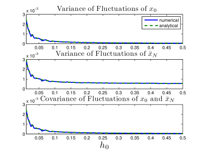
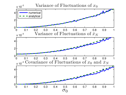
Figure 1. We compare the analytical formulas for variances and covariances with direct numerical simulations. On the left the horizontal axis is $h_{0}$ and on the right $\sigma_{0}$.

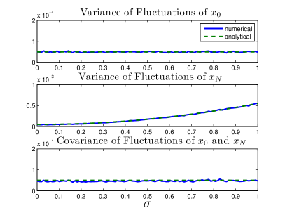
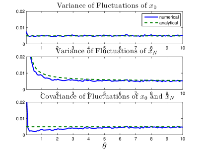
Figure 2. Same and in Figure 1 except that the horizontal axis on the left is $\sigma$ and on the right $\theta$.

6.2. Numerical results of large deviations

In this subsection, we compute the most probable paths $(x_{0},\bar{x})$, defined in Section 3.2, by numerically solving the associated boundary value problems (26) and (34) for $\sigma_{0}=0$ and $\sigma_{0}>0$, respectively. We use the boundary value problem solver bvp4c in MATLAB to solve these problems. The details of the algorithm can be found in [19].

For the non-singular cases, for $h_{0}$ small, we use $x_{0}(t)\equiv-1$ or $x_{0}(t)=(2t/T)-1$ for (26), and $x_{0}(t)=\bar{x}(t)\equiv-1$ or $x_{0}(t)=\bar{x}(t)=(2t/T)-1$ for (34), depending on which one gives better results. We found that bvp4c sometimes did not give an accurate solution even for the non-singular cases. The numerical solutions failed to pass their internal accuracy check of the MATLAB routine. The reason for this is not clear. However, this issue can be bypassed by iterating bvp4c several times. More precisely, we use the inaccurate solution as a new initial guess and use bvp4c to solve the same boundary value problem again to obtain a new solution and so on. After several iterations, bvp4c finds the correct solution that passes its accuracy check.

For the nearly-singular case, when $h_{0}$ is large, the method just described fails to find the correct solutions even with several iterations. To get past this issue, we use as initial guesses solutions of the less singular cases obtained by the above technique. For example, we use the solution of the problem with $h_{0}=1$ as an initial guess to solve the problem with $h_{0}=2$, and so on. Eventually we can solve some quite singular problems, for example, with $h_{0}=10$.

6.2.1. Impact of $h_{0}$

In Figure 3 we plot the most probable paths $(x_{0},\bar{x})$ as functions of time, for $h_{0}$ from $0$ to $10$. On the left all the plots are with $\sigma_{0}=0$ and on the right $\sigma_{0}=0.5$. We note that when $h_{0}=0$, $(x_{0},\bar{x})$ is smooth and in fact it is approximately linear, while $(x_{0},\bar{x})$ is quite curved for $h_{0}=10$. We see that when $x_{0}(t)\leq 0$, the destabilization of the system is driven by $\bar{x}(t)$. Indeed, $\bar{x}$ has higher external risk ($\sigma=1$) than $x_{0}(t)$ does ($\sigma_{0}=0$ or $\sigma_{0}=0.5$) and has no intrinsic stability ($h=0$), and therefore in the most probable path $\bar{x}(t)$ destabilizes $x_{0}(t)$. Nevertheless, once $x_{0}(t)>0$, the system transition is driven by $x_{0}(t)$ because the double-well potential forces $x_{0}$ to go to the failed state $1$, and $\bar{x}(t)$ is driven by $x_{0}(t)$. This effect is strengthened when $h_{0}$ is large because the double-well potential plays a more important role in that case.

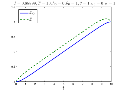
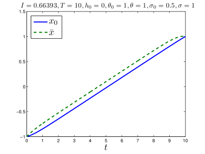
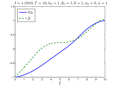
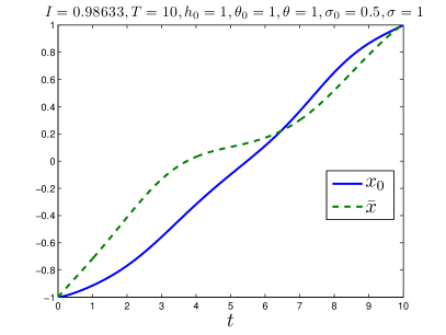
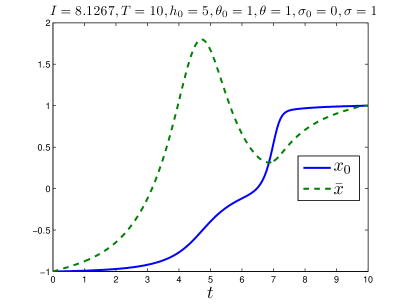
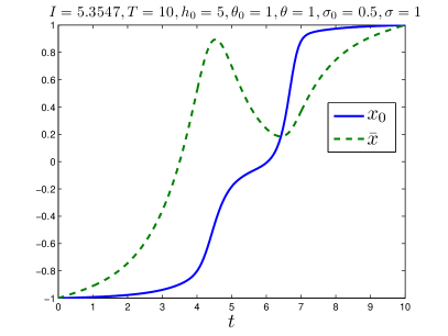
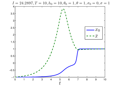
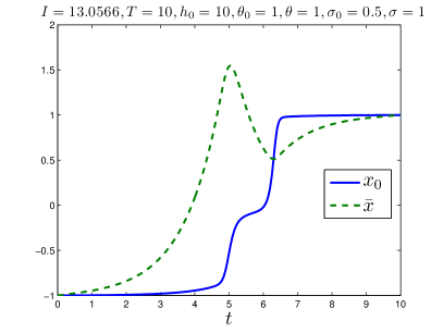
Figure 3. The most probable paths $(x_{0},\bar{x})=\arg\min_{\mathcal{A}}I$ for $h_{0}=0,1,5,10$. We let $T=10$, $\theta_{0}=1$, $\theta=1$ and $\sigma=1$. The left column is the case $\sigma_{0}=0$ and the right column is the case $\sigma_{0}=0.5$.

In Figure 4 we plot the values of $\inf_{{{\itbf x}}\in\mathcal{A}}I({{\itbf x}})$ for different $h_{0}$. We see that $\inf_{{{\itbf x}}\in\mathcal{A}}I({{\itbf x}})$ is an increasing function of $h_{0}$. This is expected because the system is more stable if it has more intrinsic stability ($h_{0}$). We also see in Figure 4 that $\inf_{{{\itbf x}}\in\mathcal{A}}I({{\itbf x}})$ has quadratic behavior with respect to $h_{0}$ for small $h_{0}$ and linear behavior for large $h_{0}$.

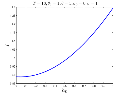
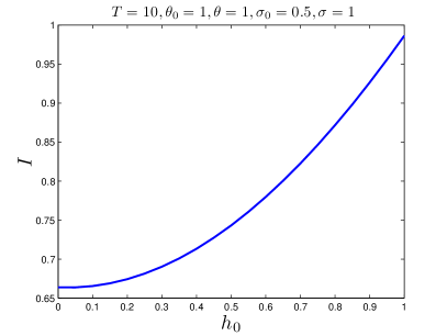
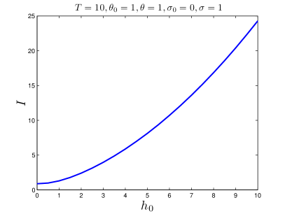
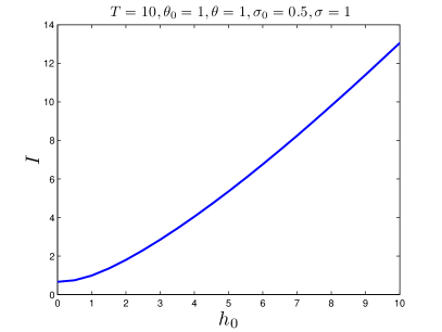
Figure 4. The infimum of $I$ over $\mathcal{A}$: $\inf_{\mathcal{A}}I$ for $h_{0}=0,0.1,0.2,\ldots,1$ and for $h_{0}=0,1,2,\ldots,10$. We let $T=10$, $\theta_{0}=1$, $\theta=1$ and $\sigma=1$. The left column is the case $\sigma_{0}=0$ and the right column is the case $\sigma_{0}=0.5$.

6.2.2. Comparison between small fluctuations and large deviations

Here we compare the small fluctuations of $(x_{0}^{(N)},\bar{x}_{N})$ described by the processes $z_{0}$ and $\bar{z}$ in (13) and the large deviations of $(x_{0}^{(N)},\bar{x}_{N})$ described by the infimum of the rate function $\inf_{{{\itbf x}}\in\mathcal{A}}I({{\itbf x}})$. For the characterization of the small fluctuations, we compute $\lim_{t\to\infty}\mathbf{Var}z_{0}(t)$ in (49) and $\lim_{t\to\infty}\mathbf{Var}\bar{z}(t)$ in (50). For the characterization of the large deviations, we compute $I(x_{0},\bar{x})$ in (23) for $\sigma_{0}=0$ where $(x_{0},\bar{x})$ is the solution of (26) and compute $I(x_{0},\bar{x})$ in (33) for $\sigma_{0}=0.5$ where $(x_{0},\bar{x})$ is the solution of (34). The goal is to visualize the fact that the systemic risk characterized by $\inf_{{{\itbf x}}\in\mathcal{A}}I({{\itbf x}})$ may vary significantly even though the individual risk measured by $\lim_{t\to\infty}\mathbf{Var}\bar{z}(t)$ is kept at a fixed level.

Motivated by (16) and (17), we know that $\lim_{t\to\infty}\mathbf{Var}z_{0}(t)$ and $\lim_{t\to\infty}\mathbf{Var}\bar{z}(t)$ are not significantly affected if we increase $\sigma$ and $\theta$ but keep the ratio $\sigma^{2}/\theta$ the same. In Figure 5 we confirm this expectation and we also observe that $\inf_{{{\itbf x}}\in\mathcal{A}}I({{\itbf x}})$ increases as $\sigma$ increases, which means that systemic risk decreases. This also means that, for a fixed level $\sigma^{2}/\theta$ of individual risk, the reduction of $\theta$, ie the interaction of the local agent with the central agent, reduces the systemic risk.

One may also expect that $\theta_{0}$ does not greatly affect $\lim_{t\to\infty}\mathbf{Var}z_{0}(t)$ and $\lim_{t\to\infty}\mathbf{Var}\bar{z}(t)$; however, in Figure 6 we see that the effect of $\theta_{0}$ on $\lim_{t\to\infty}\mathbf{Var}z_{0}(t)$ and $\lim_{t\to\infty}\mathbf{Var}\bar{z}(t)$ is not negligible. In other words, the independence of $\lim_{t\to\infty}\mathbf{Var}z_{0}(t)$ and $\lim_{t\to\infty}\mathbf{Var}\bar{z}(t)$ with respect to $\theta_{0}$ only holds in the limits (16) and (17).

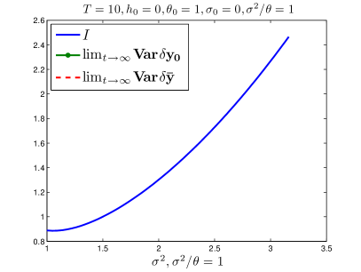
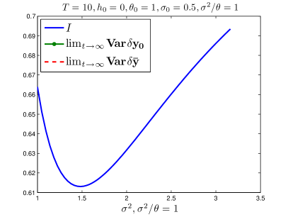
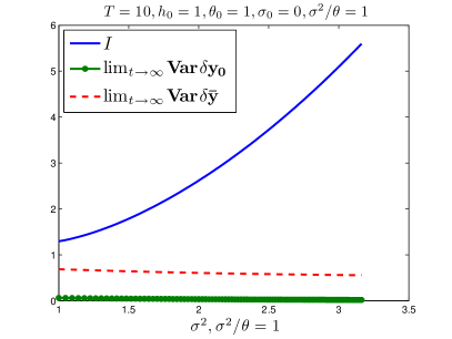
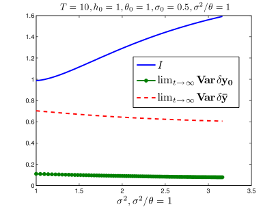
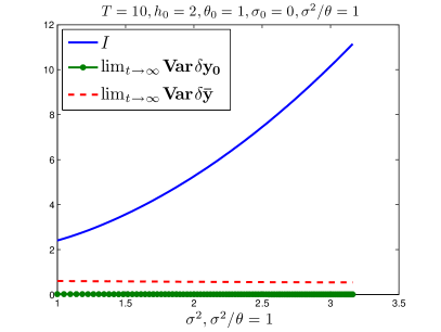
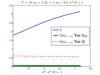
Figure 5. Plots of $\inf_{{{\itbf x}}\in\mathcal{A}}I({{\itbf x}})$, $\lim_{t\to\infty}\mathbf{Var}z_{0}(t)$ and $\lim_{t\to\infty}\mathbf{Var}\bar{z}(t)$ for $\sigma^{2}$ from $1$ to $10$ with $\sigma^{2}/\theta=1$. We let $T=10$, $\theta_{0}=1$. The left column is the case $\sigma_{0}=0$ and the right column is the case $\sigma_{0}=0.5$.

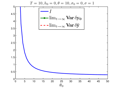
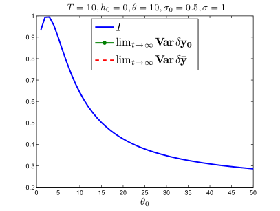
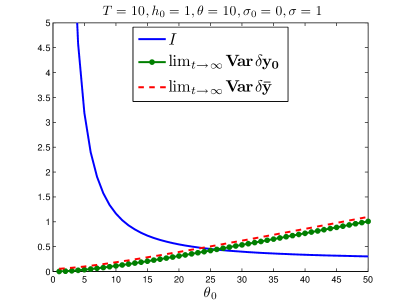
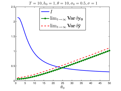
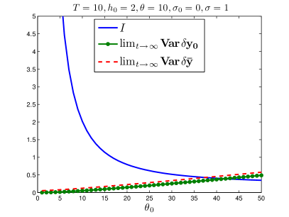
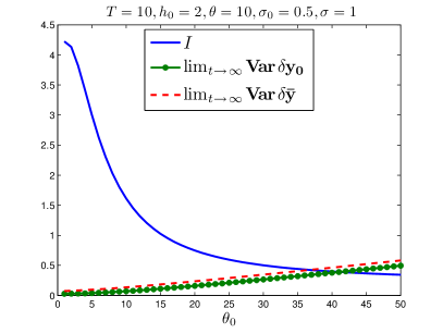
Figure 6. Plots of $\inf_{{{\itbf x}}\in\mathcal{A}}I({{\itbf x}})$, $\lim_{t\to\infty}\mathbf{Var}z_{0}(t)$ and $\lim_{t\to\infty}\mathbf{Var}\bar{z}(t)$ for $\theta_{0}$ from $1$ to $50$. We let $T=10$, $\theta=10$, $\sigma=1$. The left column is the case $\sigma_{0}=0$ and the right column is the case $\sigma_{0}=0.5$.

6.3. Numerical results for optimal controls

In this subsection, we use the Euler scheme to simulate (12) with optimal controls:

(46) $$x_{0}^{(N)}(n+1)=\frac{\sigma_{0}}{\sqrt{N}}\Delta W^{0}_{n+1}-h_{0}V_{0}^{\prime}(x_{0}^{(N)}(n))\Delta t-\theta_{0}(x_{0}^{(N)}(n)-\bar{x}_{N}(n))\Delta t,$$

$$\bar{x}_{N}(n+1)=\frac{\sigma}{\sqrt{N}}\Delta\bar{W}_{n+1}-\theta(\bar{x}_{N}(n)-x_{0}^{(N)}(n))\Delta t+\alpha_{j}^{\infty}(n)\Delta t$$

with $x_{0}^{(N)}(0)=\bar{x}_{N}(0)=-1$ and $\{\Delta W^{0}_{n+1}\}_{n}$, $\{\Delta\bar{W}_{n+1}\}_{n}$ i.i.d. Gaussian random variables with mean $0$ and variance $\Delta t$, where

(47) $$\alpha_{j}^{\infty}(t)=-\theta_{c}\left(b_{\infty}(x_{0}^{(N)}(n)+1)+d_{\infty}(x_{j}(n)+1)+e_{\infty}(\bar{x}_{N}(n)+1)\right)$$

and $(a_{\infty},b_{\infty},d_{\infty},e_{\infty})$ satisfies the algebraic Riccati equations (44).

To obtain $(a_{\infty},b_{\infty},d_{\infty},e_{\infty})$, we numerically solve (42) for large enough $T$ so that $(a(0),b(0),d(0),e(0))$ is essentially $(a_{\infty},b_{\infty},d_{\infty},e_{\infty})$. The values of the parameters used in (46) are listed in Table 2.

We see from Figure 7 that the uncontrolled problem is very unstable in the sense that $x_{0}^{(N)}$ and $\bar{x}_{N}$ jump frequently between $-1$ and $+1$. On the other hand, under the same values of the parameters, the controlled $x_{0}^{(N)}$ and $\bar{x}_{N}$ are much more stable with no transition from $-1$ to $+1$.

$N$	$T$	$\Delta t$	$h_{0}$	$\sigma_{0}$	$\theta_{0}$	$\sigma$	$\theta$
$100$	$10^{3}$	$10^{-2}$	$0.7$	$0.5$	$1.0$	$5.0$	$1.0$

Table 2. The values of the parameters used in Sec. 6.3 for the controlled problem (46) and the uncontrolled problem (45).

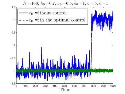
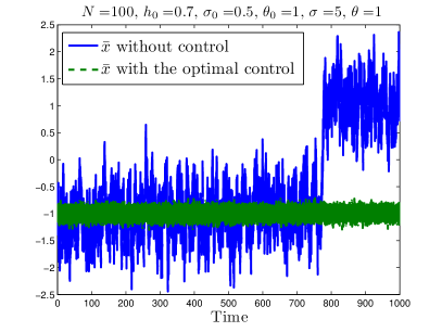
Figure 7. Sample paths of $x_{0}^{(N)}(t)$ and $\bar{x}_{N}(t)$ with and without the optimal control. With the optimal control, $x_{0}^{(N)}(t)$ and $\bar{x}_{N}(t)$ are much more stable than the uncontrolled ones.

7. Summary and Conclusions

We have formulated and analyzed a multi-agent model for the evolution of individual and systemic risk when there is a central agent acting as a stabilizer in the system. The local agents do not have an intrisinc stabilizing mechanism. The main result of this paper can be visualized in Figures 5 and 6 and is briefly described as follows. The systemic risk decreases when the rate of adherence of the local agents to the central agent increases, but it increases when the rate of adherence of the central agent to the mean of the local agents increases. This is under the condition that the observed individual risk is kept approximately constant. We also show that the effect of drift controls on the local agents is to always stabilize the systemic risk.

Appendix A Proofs in Section 3

A.1. Proof of Proposition 1

We first consider the eigen-decomposition of ${\bf A}$: ${\bf A}={\bf Q}{\boldsymbol{\Lambda}}{\bf Q}^{-1}$, where

$${\boldsymbol{\Lambda}}=\begin{pmatrix}\lambda_{1}&0\\ 0&\lambda_{2}\end{pmatrix},\quad{\bf Q}=\frac{\theta}{\lambda_{1}-\lambda_{2}}\begin{pmatrix}1+\frac{\lambda_{1}}{\theta}&1+\frac{\lambda_{2}}{\theta}\\ 1&1\end{pmatrix},\quad{\bf Q}^{-1}=\begin{pmatrix}1&-(1+\frac{\lambda_{2}}{\theta})\\ -1&1+\frac{\lambda_{1}}{\theta}\end{pmatrix},$$

$$\lambda_{1}=\frac{1}{2}\left\{-[h_{0}V_{0}^{\prime\prime}(y_{0}^{e})+\theta_{0}+\theta]+\sqrt{[h_{0}V_{0}^{\prime\prime}(y_{0}^{e})+\theta_{0}+\theta]^{2}-4\theta h_{0}V_{0}^{\prime\prime}(y_{0}^{e})}\right\},$$

$$\lambda_{2}=\frac{1}{2}\left\{-[h_{0}V_{0}^{\prime\prime}(y_{0}^{e})+\theta_{0}+\theta]-\sqrt{[h_{0}V_{0}^{\prime\prime}(y_{0}^{e})+\theta_{0}+\theta]^{2}-4\theta h_{0}V_{0}^{\prime\prime}(y_{0}^{e})}\right\}.$$

We note that $\lambda_{1}$ and $\lambda_{2}$ are real and negative if $h_{0}$, $\theta_{0}$ and $\theta$ are positive. Then from (14), $\lim_{t\to\infty}z_{0}(t)=\lim_{t\to\infty}\bar{z}(t)=0$. In addition, from the eigen-decomposition we have

(48) $$\begin{pmatrix}\mathbf{Var}z_{0}(t)&\mathbf{Cov}(z_{0}(t),\bar{z}(t))\\ \mathbf{Cov}(z_{0}(t),\bar{z}(t))&\mathbf{Var}\bar{z}(t)\end{pmatrix}\\ ={\bf Q}\int_{0}^{t}e^{(t-s){\boldsymbol{\Lambda}}}{\bf Q}^{-1}\begin{pmatrix}\sigma_{0}^{2}&0\\ 0&\sigma^{2}\end{pmatrix}({\bf Q}^{-1})^{\mathbf{T}}e^{(t-s){\boldsymbol{\Lambda}}}ds{\bf Q}^{\mathbf{T}}.$$

We observe that

$${\bf Q}^{-1}\begin{pmatrix}\sigma_{0}^{2}&0\\ 0&\sigma^{2}\end{pmatrix}({\bf Q}^{-1})^{\mathbf{T}}\\ =\begin{pmatrix}\sigma_{0}^{2}+\sigma^{2}(1+\frac{\lambda_{2}}{\theta})^{2}&-\sigma_{0}^{2}-\sigma^{2}(1+\frac{\lambda_{1}}{\theta})(1+\frac{\lambda_{2}}{\theta})\\ -\sigma_{0}^{2}-\sigma^{2}(1+\frac{\lambda_{1}}{\theta})(1+\frac{\lambda_{2}}{\theta})&\sigma_{0}^{2}+\sigma^{2}(1+\frac{\lambda_{1}}{\theta})^{2}\end{pmatrix}.$$

Then

$$\lim_{t\to\infty}\int_{0}^{t}e^{(t-s){\boldsymbol{\Lambda}}}{\bf Q}^{-1}\begin{pmatrix}\sigma_{0}^{2}&0\\ 0&\sigma^{2}\end{pmatrix}({\bf Q}^{-1})^{\mathbf{T}}e^{(t-s){\boldsymbol{\Lambda}}}ds\\ =\begin{pmatrix}-\frac{1}{2\lambda_{1}}[\sigma_{0}^{2}+\sigma^{2}(1+\frac{\lambda_{2}}{\theta})^{2}]&\frac{1}{\lambda_{1}+\lambda_{2}}[-\sigma_{0}^{2}-\sigma^{2}(1+\frac{\lambda_{1}}{\theta})(1+\frac{\lambda_{2}}{\theta})]\\ \frac{1}{\lambda_{1}+\lambda_{2}}[-\sigma_{0}^{2}-\sigma^{2}(1+\frac{\lambda_{1}}{\theta})(1+\frac{\lambda_{2}}{\theta})]&-\frac{1}{2\lambda_{2}}[\sigma_{0}^{2}+\sigma^{2}(1+\frac{\lambda_{1}}{\theta})^{2}]\end{pmatrix}.$$

So we obtain

(49) $$\lim_{t\to\infty}\mathbf{Var}z_{0}(t)=\frac{\theta^{2}}{(\lambda_{1}-\lambda_{2})^{2}}\left\{-\frac{1}{2\lambda_{1}}\left(1+\frac{\lambda_{1}}{\theta}\right)^{2}\left[\sigma_{0}^{2}+\sigma^{2}\left(1+\frac{\lambda_{2}}{\theta}\right)^{2}\right]\right.$$

$$\quad+\frac{2}{\lambda_{1}+\lambda_{2}}\left(1+\frac{\lambda_{1}}{\theta}\right)\left(1+\frac{\lambda_{2}}{\theta}\right)\left[\sigma_{0}^{2}+\sigma^{2}\left(1+\frac{\lambda_{1}}{\theta}\right)\left(1+\frac{\lambda_{2}}{\theta}\right)\right]$$

$$\quad\left.-\frac{1}{2\lambda_{2}}\left(1+\frac{\lambda_{2}}{\theta}\right)^{2}\left[\sigma_{0}^{2}+\sigma^{2}\left(1+\frac{\lambda_{1}}{\theta}\right)^{2}\right]\right\},$$

(50) $$\lim_{t\to\infty}\mathbf{Var}\bar{z}(t)=\frac{\theta^{2}}{(\lambda_{1}-\lambda_{2})^{2}}\left\{-\frac{1}{2\lambda_{1}}\left[\sigma_{0}^{2}+\sigma^{2}\left(1+\frac{\lambda_{2}}{\theta}\right)^{2}\right]\right.$$

$$\left.\quad+\frac{2}{\lambda_{1}+\lambda_{2}}\left[\sigma_{0}^{2}+\sigma^{2}\left(1+\frac{\lambda_{1}}{\theta}\right)\left(1+\frac{\lambda_{2}}{\theta}\right)\right]-\frac{1}{2\lambda_{2}}\left[\sigma_{0}^{2}+\sigma^{2}\left(1+\frac{\lambda_{1}}{\theta}\right)^{2}\right]\right\},$$

(51) $$\lim_{t\to\infty}\mathbf{Cov}(z_{0}(t),\bar{z}(t))=\frac{\theta^{2}}{(\lambda_{1}-\lambda_{2})^{2}}\left\{-\frac{1}{2\lambda_{1}}\left(1+\frac{\lambda_{1}}{\theta}\right)\left[\sigma_{0}^{2}+\sigma^{2}\left(1+\frac{\lambda_{2}}{\theta}\right)^{2}\right]\right.$$

$$\quad+\frac{1}{\lambda_{1}+\lambda_{2}}\left(1+\frac{\lambda_{1}}{\theta}\right)\left[\sigma_{0}^{2}+\sigma^{2}\left(1+\frac{\lambda_{1}}{\theta}\right)\left(1+\frac{\lambda_{2}}{\theta}\right)\right]$$

$$\quad+\frac{1}{\lambda_{1}+\lambda_{2}}\left(1+\frac{\lambda_{2}}{\theta}\right)\left[\sigma_{0}^{2}+\sigma^{2}\left(1+\frac{\lambda_{1}}{\theta}\right)\left(1+\frac{\lambda_{2}}{\theta}\right)\right]$$

$$\quad\left.-\frac{1}{2\lambda_{2}}\left(1+\frac{\lambda_{2}}{\theta}\right)\left[\sigma_{0}^{2}+\sigma^{2}\left(1+\frac{\lambda_{1}}{\theta}\right)^{2}\right]\right\}.$$

We are interested in the case that $\sigma$ and $\theta$ go to infinity while the ratio $\alpha=\sigma^{2}/\theta$ is fixed. For $\theta$ large and using the approximation $\sqrt{1+x}=1+\frac{1}{2}x+O(x^{2})$, we have the following expansions:

$$\frac{\lambda_{1}}{\theta} =\frac{1}{2\theta}\left\{-[h_{0}V_{0}^{\prime\prime}(y_{0}^{e})+\theta_{0}+\theta]+[h_{0}V_{0}^{\prime\prime}(y_{0}^{e})+\theta_{0}+\theta]\sqrt{1-\frac{4\theta h_{0}V_{0}^{\prime\prime}(y_{0}^{e})}{[h_{0}V_{0}^{\prime\prime}(y_{0}^{e})+\theta_{0}+\theta]^{2}}}\right\}$$

$$=-\frac{h_{0}V_{0}^{\prime\prime}(y_{0}^{e})}{h_{0}V_{0}^{\prime\prime}(y_{0}^{e})+\theta_{0}+\theta}+O\left(\frac{1}{\theta^{2}}\right),$$

$$1+\frac{\lambda_{2}}{\theta} =\frac{1}{2\theta}\left\{2\theta-[h_{0}V_{0}^{\prime\prime}(y_{0}^{e})+\theta_{0}+\theta]-[h_{0}V_{0}^{\prime\prime}(y_{0}^{e})+\theta_{0}+\theta]\sqrt{1-\frac{4\theta h_{0}V_{0}^{\prime\prime}(y_{0}^{e})}{[h_{0}V_{0}^{\prime\prime}(y_{0}^{e})+\theta_{0}+\theta]^{2}}}\right\}$$

$$=-\frac{1}{\theta}[h_{0}V_{0}^{\prime\prime}(y_{0}^{e})+\theta_{0}]+\frac{h_{0}V_{0}^{\prime\prime}(y_{0}^{e})}{h_{0}V_{0}^{\prime\prime}(y_{0}^{e})+\theta_{0}+\theta}+O\left(\frac{1}{\theta^{2}}\right).$$

Thus $\lambda_{1}\to h_{0}V_{0}^{\prime\prime}(y_{0}^{e})$ as $\theta\to\infty$ and $1+\frac{\lambda_{2}}{\theta}=O(\frac{1}{\theta})$ and finally we have the limits (16), (17) and (18).

A.2. Proof of Proposition 2

If $x_{0}$ is the minimizer, then for any perturbation $\phi$ with $\phi(0)=\phi(T)=\dot{\phi}(0)=\dot{\phi}(T)=0$, the directional derivative of $I$ must be zero:

$$\left.\frac{d}{d\epsilon}\right|_{\epsilon=0}I(x_{0}+\epsilon\phi)=\frac{1}{2\sigma^{2}}\int_{0}^{T}2\left[\frac{1}{\theta_{0}}\ddot{x}_{0}+\frac{h_{0}}{\theta_{0}}V^{\prime\prime}_{0}(x_{0})\dot{x}_{0}+\left(1+\frac{\theta}{\theta_{0}}\right)\dot{x}_{0}+\frac{\theta h_{0}}{\theta_{0}}V^{\prime}_{0}(x_{0})\right]\\ \times\left[\frac{1}{\theta_{0}}\ddot{\phi}+\frac{h_{0}}{\theta_{0}}V^{\prime\prime\prime}_{0}(x_{0})\phi\dot{x}_{0}+\frac{h_{0}}{\theta_{0}}V^{\prime\prime}_{0}(x_{0})\dot{\phi}+\left(1+\frac{\theta}{\theta_{0}}\right)\dot{\phi}+\frac{\theta h_{0}}{\theta_{0}}V^{\prime\prime}_{0}(x_{0})\phi\right]dt=0.$$

After integration by parts and using the fact that $\phi$ is arbitrary, the minimizer $x_{0}$ must satisfy the following equation:

$$\frac{1}{\theta_{0}}\frac{d^{2}}{dt^{2}}\left[\frac{1}{\theta_{0}}\ddot{x}_{0}+\frac{h_{0}}{\theta_{0}}V^{\prime\prime}_{0}(x_{0})\dot{x}_{0}+\left(1+\frac{\theta}{\theta_{0}}\right)\dot{x}_{0}+\frac{\theta h_{0}}{\theta_{0}}V^{\prime}_{0}(x_{0})\right]$$

$$+\frac{h_{0}}{\theta_{0}}V^{\prime\prime\prime}_{0}(x_{0})\dot{x}_{0}\left[\frac{1}{\theta_{0}}\ddot{x}_{0}+\frac{h_{0}}{\theta_{0}}V^{\prime\prime}_{0}(x_{0})\dot{x}_{0}+\left(1+\frac{\theta}{\theta_{0}}\right)\dot{x}_{0}+\frac{\theta h_{0}}{\theta_{0}}V^{\prime}_{0}(x_{0})\right]$$

$$-\frac{d}{dt}\left\{\frac{h_{0}}{\theta_{0}}V^{\prime\prime}_{0}(x_{0})\left[\frac{1}{\theta_{0}}\ddot{x}_{0}+\frac{h_{0}}{\theta_{0}}V^{\prime\prime}_{0}(x_{0})\dot{x}_{0}+\left(1+\frac{\theta}{\theta_{0}}\right)\dot{x}_{0}+\frac{\theta h_{0}}{\theta_{0}}V^{\prime}_{0}(x_{0})\right]\right\}$$

$$-\left(1+\frac{\theta}{\theta_{0}}\right)\frac{d}{dt}\left[\frac{1}{\theta_{0}}\ddot{x}_{0}+\frac{h_{0}}{\theta_{0}}V^{\prime\prime}_{0}(x_{0})\dot{x}_{0}+\left(1+\frac{\theta}{\theta_{0}}\right)\dot{x}_{0}+\frac{\theta h_{0}}{\theta_{0}}V^{\prime}_{0}(x_{0})\right]$$

$$+\frac{\theta h_{0}}{\theta_{0}}V^{\prime\prime}_{0}(x_{0})\left[\frac{1}{\theta_{0}}\ddot{x}_{0}+\frac{h_{0}}{\theta_{0}}V^{\prime\prime}_{0}(x_{0})\dot{x}_{0}+\left(1+\frac{\theta}{\theta_{0}}\right)\dot{x}_{0}+\frac{\theta h_{0}}{\theta_{0}}V^{\prime}_{0}(x_{0})\right] =0.$$

with the boundary conditions $x_{0}\left(0\right)=-1$, $x_{0}(t)=1$ and $\frac{d}{dt}x_{0}\left(0\right)=\frac{d}{dt}x_{0}(t)=0$. We then obtain (26) after rearranging the above equation.

A.3. Proof of Proposition 5

If $h_{0}=0$, (12) is a system of linear SDEs, and the explicit solution can be found:

$$\begin{pmatrix}x_{0}(T)\\ \bar{x}_{N}(T)\end{pmatrix}=e^{T{\bf A}_{0}}\begin{pmatrix}-1\\ -1\end{pmatrix}+\frac{1}{\sqrt{N}}\int_{0}^{T}e^{(T-s){\bf A}_{0}}\begin{pmatrix}\sigma_{0}dW_{s}^{0}\\ \sigma d\bar{W}_{s}\end{pmatrix},\quad\quad{\bf A}_{0}=\begin{pmatrix}-\theta_{0}&\theta_{0}\\ \theta&-\theta\end{pmatrix}.$$

Since (12) is linear, $(x_{0}(T),\bar{x}_{N}(T))$ is jointly Gaussian and can be completely characterized by its mean and covariance matrix. We note that $(-1,-1)^{\mathbf{T}}$ is in the null space of ${\bf A}_{0}$ and thus

$$\mathbb{E}\begin{pmatrix}x_{0}(T)\\ \bar{x}_{N}(T)\end{pmatrix}=e^{T{\bf A}_{0}}\begin{pmatrix}-1\\ -1\end{pmatrix}=\begin{pmatrix}-1\\ -1\end{pmatrix}.$$

In addition, ${\bf A}_{0}$ has the following eigen-decomposition: ${\bf A}_{0}={\bf Q}_{0}{\boldsymbol{\Lambda}}_{0}{\bf Q}_{0}^{-1}$, where

$${\boldsymbol{\Lambda}}_{0}=\begin{pmatrix}0&0\\ 0&-(\theta_{0}+\theta)\end{pmatrix},\quad{\bf Q}_{0}=\frac{\theta}{\theta_{0}+\theta}\begin{pmatrix}1&-\frac{\theta_{0}}{\theta}\\ 1&1\end{pmatrix},\quad{\bf Q}^{-1}_{0}=\begin{pmatrix}1&\frac{\theta_{0}}{\theta}\\ -1&1\end{pmatrix}.$$

Then the covariance matrix is

(52) $$\begin{pmatrix}\mathbf{Var}x_{0}(T)&\mathbf{Cov}(x_{0}(T),\bar{x}(T))\\ \mathbf{Cov}(x_{0}(T),\bar{x}(T))&\mathbf{Var}\bar{x}(T)\end{pmatrix}$$

$$=\frac{1}{N}{\bf Q}_{0}\int_{0}^{T}e^{(T-s){\boldsymbol{\Lambda}}_{0}}{\bf Q}_{0}^{-1}\begin{pmatrix}\sigma_{0}^{2}&0\\ 0&\sigma^{2}\end{pmatrix}({\bf Q}_{0}^{-1})^{\mathbf{T}}e^{(T-s){\boldsymbol{\Lambda}}_{0}}ds{\bf Q}_{0}^{\mathbf{T}}$$

$$=\frac{1}{N}{\bf Q}_{0}{\boldsymbol{\Sigma}}{\bf Q}_{0}^{\mathbf{T}},$$

with

$${\boldsymbol{\Sigma}}=\begin{pmatrix}T(\sigma_{0}^{2}+\theta_{0}^{2}\sigma^{2}/\theta^{2})&\frac{1}{\theta_{0}+\theta}(-\sigma_{0}^{2}+\theta_{0}\sigma^{2}/\theta)[1-e^{-T(\theta_{0}+\theta)}]\\ \frac{1}{\theta_{0}+\theta}(-\sigma_{0}^{2}+\theta_{0}\sigma^{2}/\theta)[1-e^{-T(\theta_{0}+\theta)}]&\frac{1}{2(\theta_{0}+\theta)}(\sigma_{0}^{2}+\sigma^{2})[1-e^{-2T(\theta_{0}+\theta)}]\end{pmatrix}.$$

When the terminal time $T$ is large, we can separate the middle matrix in (52) into the principle term and the correction term:

$${\boldsymbol{\Sigma}}=\begin{pmatrix}T(\sigma_{0}^{2}+\theta_{0}^{2}\sigma^{2}/\theta^{2})&0\\ 0&0\end{pmatrix}$$

$$+\begin{pmatrix}0&\frac{1}{\theta_{0}+\theta}(-\sigma_{0}^{2}+\theta_{0}\sigma^{2}/\theta)[1-e^{-T(\theta_{0}+\theta)}]\\ \frac{1}{\theta_{0}+\theta}(-\sigma_{0}^{2}+\theta_{0}\sigma^{2}/\theta)[1-e^{-T(\theta_{0}+\theta)}]&\frac{1}{2(\theta_{0}+\theta)}(\sigma_{0}^{2}+\sigma^{2})[1-e^{-2T(\theta_{0}+\theta)}]\end{pmatrix}.$$

Then we have the approximation of the covariance matrix:

(53) $$\begin{pmatrix}\mathbf{Var}x_{0}(T)&\mathbf{Cov}(x_{0}(T),\bar{x}(T))\\ \mathbf{Cov}(x_{0}(T),\bar{x}(T))&\mathbf{Var}\bar{x}(T)\end{pmatrix} \approx\frac{1}{N}{\bf Q}_{0}\begin{pmatrix}T(\sigma_{0}^{2}+\theta_{0}^{2}\sigma^{2}/\theta^{2})&0\\ 0&0\end{pmatrix}{\bf Q}_{0}^{\mathbf{T}}$$

$$=\frac{T}{N}\frac{\theta^{2}\sigma_{0}^{2}+\theta_{0}^{2}\sigma^{2}}{(\theta_{0}+\theta)^{2}}\begin{pmatrix}1&1\\ 1&1\end{pmatrix}.$$

From (53) we conclude that $x_{0}(T)$ and $\bar{x}(T)$ are approximately equal as $T$ becomes large and the probability in (35) is approximately $\mathbb{P}(x_{0}(T)\in(1,1+dx))$, which gives the desired rate of decay by using the fact that $x_{0}(T)$ is Gaussian with mean $-1$ and approximate variance $\mathbf{Var}x_{0}(T)$ in (53) for large $T$.

Appendix B Proof of Proposition 6

We prove it in three steps. The first step is to show that there exists a uniform lower bound for $\mathcal{J}$ over all feasible $\phi$.

Lemma 8.

If $h=0$, then for all $\phi(t,dx)$ such that $\langle\phi(t,dx),x\rangle=\bar{x}(t)$,

$$\mathcal{J}\big{(}(x_{0}(t),\phi(t,dx))_{t\in[0,T]}\big{)} \geq \frac{1}{2\sigma_{0}^{2}}\int_{0}^{T}(\dot{x}_{0}+h_{0}V_{0}^{\prime}(x_{0})+\theta_{0}(x_{0}-\bar{x}))^{2}dt$$

$$+\frac{1}{2\sigma^{2}}\int_{0}^{T}(\dot{\bar{x}}+\theta(\bar{x}-x_{0}))^{2}dt,$$

for $\sigma_{0}>0$ and for $\sigma_{0}=0$,

$$\mathcal{J}\big{(}(x_{0}(t),\phi(t,dx))_{t\in[0,T]}\big{)}\geq\frac{1}{2\sigma^{2}}\int_{0}^{T}(\dot{\bar{x}}+\theta(\bar{x}-x_{0}))^{2}dt,$$

if $\dot{x}_{0}+h_{0}V_{0}^{\prime}(x_{0})+\theta_{0}(x_{0}-\bar{x})=0$ or $\mathcal{J}\big{(}(x_{0}(t),\phi(t,dx))_{t\in[0,T]}\big{)}=\infty$ otherwise.

Proof.

By taking $f(x)=x$, we have

$$\int_{0}^{T}\sup_{f(x):\langle\phi,(f^{\prime}(x))^{2}\rangle\neq 0}\frac{\langle\phi_{t}-\frac{1}{2}\sigma^{2}\phi_{xx}-\theta\frac{\partial}{\partial x}[(x-x_{0}(t))\phi],f(x)\rangle^{2}}{\langle\phi,(f^{\prime}(x))^{2}\rangle}dt\\ \overset{f(x)=x}{\geq}\int_{0}^{T}\frac{\langle\phi_{t}-\frac{1}{2}\sigma^{2}\phi_{xx}-\theta\frac{\partial}{\partial x}[(x-x_{0}(t))\phi],x\rangle^{2}}{\langle\phi,1\rangle}dt=\int_{0}^{T}(\dot{\bar{x}}+\theta(\bar{x}-x_{0}))^{2}dt.$$

Then we have the desired results. ∎

We then prove that $\mathcal{J}\big{(}(x_{0}(t),\bar{p}(t,dx))_{t\in[0,T]}\big{)}=I\big{(}(x_{0}(t),\bar{x}(t))_{\in[0,T]}\big{)}$ and consequently $\mathcal{I}(x_{0},\bar{x})=I(x_{0},\bar{x})$.

Lemma 9.

Let $\bar{p}$ defined in (37) and $h=0$. Then $\mathcal{J}\big{(}(x_{0}(t),\bar{p}(t,dx))_{t\in[0,T]}\big{)}=I(x_{0},\bar{x})$ in (23) for $\sigma_{0}=0$ and $\mathcal{J}\big{(}(x_{0}(t),\bar{p}(t,dx))_{t\in[0,T]}\big{)}=I(x_{0},\bar{x})$ in (33) for $\sigma_{0}>0$. Consequently, $\bar{p}(t,dx)$ is a minimizer and $\mathcal{I}(x_{0},\bar{x})=I(x_{0},\bar{x})$ for either $\sigma_{0}=0$ or $\sigma_{0}>0$.

Proof.

By using the same argument in [10, Proposition 5.3], if $\phi(t,dx)$ is absolutely continuous with respect to the Lebesgue measure with the smooth density function $\phi(t,x)$, then

$$\int_{0}^{T}\sup_{f(x):\langle\phi,(f^{\prime}(x))^{2}\rangle\neq 0}\frac{\langle\phi_{t}-\frac{1}{2}\sigma^{2}\phi_{xx}-\theta\frac{\partial}{\partial x}[(x-x_{0}(t))\phi],f(x)\rangle^{2}}{\langle\phi,(f^{\prime}(x))^{2}\rangle}dt=\int_{0}^{T}\langle\phi,(g(t,x))^{2}\rangle dt,$$

where $g(t,x)$ satisfies

$$\phi_{t}(t,x)-\frac{1}{2}\sigma^{2}\phi_{xx}(t,x)-\theta\frac{\partial}{\partial x}[(x-x_{0}(t))\phi(t,x)]=\frac{\partial}{\partial x}(\phi(t,x)g(t,x)).$$

If $\phi(t,x)=\bar{p}(t,x)$, then by using the fact that $\bar{p}_{t}=-\dot{\bar{x}}(t)\bar{p}_{x}$ and $\frac{1}{2}\sigma^{2}\bar{p}_{xx}+\theta\frac{\partial}{\partial x}[(x-x_{0}(t))\bar{p}]=\theta[(\bar{x}(t)-x_{0}(t))\bar{p}_{x}]$, the corresponding $g(t,x)$ satisfies

$$-\dot{\bar{x}}(t)\bar{p}_{x}-\theta[(\bar{x}(t)-x_{0}(t))\bar{p}_{x}]=\frac{\partial}{\partial x}(g(t,x)\bar{p}).$$

Then $g(t,x)=-\dot{\bar{x}}(t)-\theta(\bar{x}(t)-x_{0}(t))$ and $\int_{0}^{T}\langle\phi,(g(t,x))^{2}\rangle dt=\int_{0}^{T}(\dot{\bar{x}}(t)+\theta(\bar{x}(t)-x_{0}(t)))^{2}dt$. We therefore obtain the desired results. ∎

Finally we show that the minimizer $(\bar{p}(t,dx))_{t\in[0,T]}$ is unique.

Lemma 10.

The minimizer $(\bar{p}(t,dx))_{t\in[0,T]}$ of $\inf_{\phi(t,dx)}\mathcal{J}\big{(}(x_{0}(t),\phi(t,dx))_{t\in[0,T]}\big{)}$ is unique for all $(\phi(t,dx))_{t\in[0,T]}$ such that $\langle\phi(t,dx),x\rangle=\bar{x}(t)$ for all $t\in[0,T]$ and $\phi(0,dx)=\bar{p}(0,dx)$.

Proof.

From the previous lemmas we conclude that if $(\phi(t,dx))_{t\in[0,T]}$ is a minimizer, then

$$x=\underset{f(x):\langle\phi,(f^{\prime}(x))^{2}\rangle\neq 0}{\arg\sup}\frac{\langle\phi_{t}-\frac{1}{2}\sigma^{2}\phi_{xx}-\theta\frac{\partial}{\partial x}[(x-x_{0}(t))\phi],f(x)\rangle^{2}}{\langle\phi,(f^{\prime}(x))^{2}\rangle}.$$

Therefore for any perturbation $\hat{f}(x)$,

$$\left.\frac{d}{d\epsilon}\right|_{\epsilon=0}\frac{\langle\phi_{t}-\frac{1}{2}\sigma^{2}\phi_{xx}-\theta\frac{\partial}{\partial x}[(x-x_{0}(t))\phi],x+\epsilon\hat{f}(x)\rangle^{2}}{\langle\phi,(1+\epsilon\hat{f}^{\prime}(x))^{2}\rangle}=0,$$

which leads to

$$\phi_{t}-\frac{1}{2}\sigma^{2}\phi_{xx}-\theta\frac{\partial}{\partial x}[(x-x_{0}(t))\phi] =\langle\phi_{t}-\frac{1}{2}\sigma^{2}\phi_{xx}-\theta\frac{\partial}{\partial x}[(x-x_{0}(t))\phi],x\rangle\phi$$

$$=[\dot{\bar{x}}(t)+\theta(\bar{x}(t)-x_{0}(t))]\phi.$$

In other words, a minimizer $(\phi(t,dx))_{t\in[0,T]}$ must satisfy the above linear parabolic PDE that has a unique solution with the given initial condition $\phi(0,dx)=\bar{p}(0,dx)$. ∎

Appendix C Proof of Proposition 7

We can rewrite the problem in the matrix form:

$$\min_{({\boldsymbol{\alpha}}(t))_{t\in[0,T]}}\frac{1}{2}\mathbb{E}\left[\int_{0}^{T}{\boldsymbol{\alpha}}(t)^{\mathbf{T}}\mathbf{R}{\boldsymbol{\alpha}}(t)+{{\itbf X}}(t)^{\mathbf{T}}\mathbf{Q}{{\itbf X}}(t)dt\right],\quad d{{\itbf X}}=\mathbf{\Sigma}d{{\itbf W}}+\mathbf{A}{{\itbf X}}+\mathbf{B}{\boldsymbol{\alpha}}dt,$$

where

$$\mathbf{\Sigma}=\begin{pmatrix}\frac{\sigma_{0}}{\sqrt{N}}&0{\itbf u}^{\mathbf{T}}\\ 0{\itbf u}&\sigma\mathbf{I}\end{pmatrix},\quad\mathbf{A}=\begin{pmatrix}-\theta_{0}-H_{0}&\frac{\theta_{0}}{N}{\itbf u}^{\mathbf{T}}\\ \theta{\itbf u}&-\theta\mathbf{I}\end{pmatrix},\quad\mathbf{B}=\begin{pmatrix}0&0{\itbf u}^{\mathbf{T}}\\ 0{\itbf u}&\mathbf{I}\end{pmatrix},$$

$$\mathbf{Q}=\theta_{c}\begin{pmatrix}N&-{\itbf u}^{\mathbf{T}}\\ -{\itbf u}&\mathbf{I}\end{pmatrix},\quad\mathbf{R}=\frac{1}{\theta_{c}}\begin{pmatrix}1&0{\itbf u}^{\mathbf{T}}\\ 0{\itbf u}&\mathbf{I}\end{pmatrix},\quad{\itbf u}=(1,\ldots,1)^{\mathbf{T}}.$$

We apply the standard theory [24, Theorem 6.1] and we find that the optimal control is

$${\boldsymbol{\alpha}}(t)=-\mathbf{R}^{-1}\mathbf{B}^{\mathbf{T}}\mathbf{S}(t){{\itbf X}}(t)$$

where ${\bf S}(t)$ is solution of the matrix Riccati equation

$$-\frac{d}{dt}\mathbf{S}=\mathbf{A}^{\mathbf{T}}\mathbf{S}+\mathbf{S}\mathbf{A}-\mathbf{S}^{\mathbf{T}}\mathbf{B}\mathbf{R}^{-1}\mathbf{B}^{\mathbf{T}}\mathbf{S}+\mathbf{Q},$$

with the terminal condition $\mathbf{S}(T)=\mathbf{0}$. We find that

$$\mathbf{S}(t)=\begin{pmatrix}Na(t)&b(t){\itbf u}^{\mathbf{T}}\\ b(t){\itbf u}&d(t)\mathbf{I}+\frac{e(t)}{N}\mathbf{J}\end{pmatrix},$$

where $\mathbf{J}$ is the $N\times N$ matrix full of ones and $(a(t),b(t),d(t),e(t))_{t\in[0,T]}$ is the solution of

$$\dot{a}(t) =2(\theta_{0}+H_{0})a(t)-2\theta b(t)+\theta_{c}b^{2}(t)-\theta_{c},$$

$$\dot{b}(t) =(\theta_{0}+H_{0}+\theta)b(t)-\theta d(t)-\theta_{0}a(t)+\theta_{c}b(t)d(t)+\theta_{c}-\theta e(t)+\theta_{c}b(t)e(t),$$

$$\dot{d}(t) =2\theta d(t)+\theta_{c}d^{2}(t)-\theta_{c},$$

$$\dot{e}(t) =-2\theta_{0}b(t)+2\theta e(t)+\theta_{c}(2d(t)e(t)+e^{2}(t)),$$

with $(a(T),b(T),d(T),e(T))=(0,0,0,0)$. Therefore the optimal control is

$$\alpha_{j}(t)=-\theta_{c}(b(t)X_{0}(t)+d(t)X_{j}(t)+e(t)\bar{X}_{N}(t)),\quad j=1,\ldots,N.$$

References

- [1] Lijun Bo and Agostino Capponi. Systemic risk in interbanking networks. SIAM Journal on Financial Mathematics, 6(1):386–424, 2015.
- [2] A. Budhiraja, P. Dupuis, and M. Fischer. Large deviation properties of weakly interacting processes via weak convergence methods. Ann. Probab., 40(1):74–102, 2012.
- [3] Rene Carmona, Jean-Pierre Fouque, and Li-Hsien Sun. Mean field games and systemic risk. Communications in Mathematical Sciences, to appear, 2013.
- [4] Paolo Dai Pra, Wolfgang J. Runggaldier, Elena Sartori, and Marco Tolotti. Large portfolio losses: A dynamic contagion model. The Annals of Applied Probability, 19(1):pp. 347–394, 2009.
- [5] D. A. Dawson. Critical dynamics and fluctuations for a mean-field model of cooperative behavior. J. Statist. Phys., 31(1):29–85, 1983.
- [6] D. A. Dawson and J. Gärtner. Large deviations from the McKean-Vlasov limit for weakly interacting diffusions. Stochastics, 20(4):247–308, 1987.
- [7] D. A. Dawson and J. Gärtner. Large deviations, free energy functional and quasi-potential for a mean field model of interacting diffusions. Mem. Amer. Math. Soc., 78(398):iv+94, 1989.
- [8] A. Dembo and O. Zeitouni. Large deviations techniques and applications, volume 38 of Stochastic Modelling and Applied Probability. Springer-Verlag, Berlin, 2010. Corrected reprint of the second (1998) edition.
- [9] Jean-Pierre Fouque and Tomoyuki Ichiba. Stability in a model of interbank lending. SIAM Journal on Financial Mathematics, 4(1):784–803, 2013.
- [10] J. Garnier, G. Papanicolaou, and T. Yang. Large deviations for a mean field model of systemic risk. SIAM Journal on Financial Mathematics, 4(1):151–184, 2013.
- [11] Josselin Garnier, George Papanicolaou, and Tzu-Wei Yang. Diversification in financial networks may increase systemic risk. Handbook on Systemic Risk, page 432, 2013.
- [12] J. Gärtner. On the McKean-Vlasov limit for interacting diffusions. Math. Nachr., 137:197–248, 1988.
- [13] Kay Giesecke, Konstantinos Spiliopoulos, and Richard B. Sowers. Default clustering in large portfolios: Typical events. Ann. Appl. Probab., 23(1):348–385, 02 2013.
- [14] Kay Giesecke, Konstantinos Spiliopoulos, Richard B. Sowers, and Justin A. Sirignano. Large portfolio asymptotics for loss from default. Mathematical Finance, 25(1):77–114, 2015.
- [15] Tomoyuki Ichiba and Mykhaylo Shkolnikov. Large deviations for interacting bessel-like processes and applications to systemic risk. arXiv preprint arXiv:1303.3061, 2013.
- [16] Thomas G. Kurtz and Jie Xiong. Particle representations for a class of nonlinear {SPDEs}. Stochastic Processes and their Applications, 83(1):103 – 126, 1999.
- [17] Mathieu Lauriere and Olivier Pironneau. Dynamic programming for mean-field type control. Comptes Rendus Mathematique, 352(9):707–713, 2014.
- [18] S. Méléard. Asymptotic behaviour of some interacting particle systems; McKean-Vlasov and Boltzmann models. In Probabilistic models for nonlinear partial differential equations (Montecatini Terme, 1995), volume 1627 of Lecture Notes in Math., pages 42–95. Springer, Berlin, 1996.
- [19] L. F. Shampine, I. Gladwell, and S. Thompson. Solving ODEs with MATLAB. Cambridge University Press, 2003.
- [20] Konstantinos Spiliopoulos, Justin A. Sirignano, and Kay Giesecke. Fluctuation analysis for the loss from default. Stochastic Processes and their Applications, 124(7):2322 – 2362, 2014.
- [21] Konstantinos Spiliopoulos and Richard B. Sowers. Default clustering in large pools: Large deviations. SIAM Journal on Financial Mathematics, 6(1):86–116, 2015.
- [22] Alain-Sol Sznitman. Topics in propagation of chaos. volume 1464 of Lecture Notes in Mathematics, pages 165–251. Springer Berlin Heidelberg, 1991.
- [23] H. Tanaka. Limit theorems for certain diffusion processes with interaction. In Stochastic analysis (Katata/Kyoto, 1982), volume 32 of North-Holland Math. Library, pages 469–488. North-Holland, Amsterdam, 1984.
- [24] J. Yong and X. Y. Zhou. Stochastic Controls: Hamiltonian Systems and HJB Equations. Springer-Verlag, New York, 1999.