Manipulating $Z_{2}$ and Chern topological phases in a single material using periodically driving fields

Abstract

$Z_{2}$ and Chern topological phases such as newly discovered quantum spin Hall and original quantum Hall states hardly both co–exist in a single material due to their contradictory requirement on the time–reversal symmetry (TRS). We show that although the TRS is broken in systems with a periodically driving ac-field, an effective TRS can still be defined provided the ac–field is linearly polarized or certain other conditions are satisfied. The controllable TRS provides us with a route to manipulate $Z_{2}$ and Chern topological phases in a single material by tuning the polarization of the ac–field. To demonstrate the idea, we consider a generic honeycomb lattice model as a benchmark system that is relevant to electronic structures of several monolayered materials. Our calculation shows that not only the transitions between $Z_{2}$ and Chern phases can be induced but also features such as the dispersion of the edge states can be controlled. This opens the possibility of manipulating various topological phases in a single material and can be a promising approach to engineer some new electronic states of matter.

Introduction. The discovery of topological insulators (TIs) in condensed matter systems has not only revealed novel physics of the quantum world but also unified many physical phenomena, which were thought to be irreverent, into the same frameworkTI-6 . Their peculiar edge states make TIs a hot topic for both fundamental interests and industrial applications. Several materials such as HgTe/CdTe quantum well, Bi_xSb_1-x alloys, Bi₂Se₃ and Bi₂Te₃, etc., have been proven to be TIs by experimentsTI-1 . Despite these successes, how to design a topologically non–trivial material, remains a challenging issue. In most cases, the discovery of new TIs still relies on serendipity rather than predetermination.

Instead of searching for materials with intrinsically non–trivial topology, there are several recent studies focusing on manipulation of topological phases using controllable physical processes, e.g. electric fields, strains, etcTT-1 ; TT-2 ; TT-3 . Those studies not only offer new tools to generate various topological phases but also open new ways to making real electronic devices.

One of the promising methods to engineer a topological property of a system is to use periodically driving fieldsFB-1 ; FB-2 ; FB-3 ; FB-4 ; FB-5 . The proposal is based on the Floquet theory which states that the Hamiltonian of a system with a time–dependent periodic potential can be mapped into an effective static Hamiltonian, called the Floquet Hamiltonian. If the (quasi)band structure of a Floquet Hamiltonian exhibits a topological behavior, we can expect there exists a similar feature in the original Hamiltonian in a dynamical fashion. An advantage of using this method to engineer the band topology is that the ac–field provides a set of tunable parameters such that a variety of band structures unaccessible in the original material can be generated in a dynamical way. Many proposals based on the topology of Floquet Hamiltonians have appeared recently, some of which are: Floquet TIs in grapheneFTI-1 , Floquet TIs in semiconductor quantum wellsFTI-2 , Floquet Majorana fermions in topological superconductorsFTI-3 , merging Floquet Dirac pointsFTI-4 , Floquet fractional Chern insulatorsFTI-5 , Floquet Wely semimetalFTI-6 , etc. A few experiments that support the idea of Floquet TIs have also been carried outFEX-1 ; FEX-2 . Those works not only lighten up the road to manipulate topological phases but also bring us a vast landscape of new physical phenomena that are hardly found in static systems.

While many topological phases have been studied within the Floquet framework, the discussion of $Z_{2}$ phases remains scarce because time–reversal symmetry (TRS), a necessary condition for the existence of the $Z_{2}$ phase, is always broken due to the time dependence of the external perturbation. However, the Floquet Hamiltonian is merely an effective mapping of the original Hamiltonian, so the loss of TRS in original Hamiltonian does not necessarily result in the loss of TRS in Floquet Hamiltonian. Establishing an operator that links Floquet states in the Brillouin zone by a similar way as conventional TR operator does it for Bloch states, an effective TRS can be definedFTI-2 ; FB-2 . If so, two seemingly contradictory phases, TRS protected $Z_{2}$ phase, such as recently discovered quantum spin Hall state, and TRS broken Chern phase, such as much celebrated original quantum Hall state, can both be manipulated in a single material by tuning the ac–field, which is the main message of the present work.

Here, we first show how we truncate the Floquet Hamiltoian to finite dimension in a realistic calculation. Second, we show that the TRS conditions can be easily satisfied if the field is linearly polarized or certain low excitation conditions are reached. Third, we use a prototypical 2D material with strong spin–orbit coupling as a benchmark in our calculation, in order to demonstrate the idea of manipulating $Z_{2}$ and Chern topological phases in the same system. More specifically, we consider a generic half–filled $p$–orbital honeycomb lattice model to illustrate our findings. Our results show the evidence for the $Z_{2}$ phase with the ability to control the dispersion of its edge states by properly tailoring the external ac–field. When the polarization is away from the effective TRS condition, a rich Chern phase diagram begins to appear which suggests a Z₂–Chern phase transition. Thus we demonstrate the possibility of manipulating between the two topological phases in a single material which can serve as a promising tool to engineer some novel electronic states in condensed matter systems.

Floquet Theorem. We consider a tight–binding Hamiltonian with an external time perodical ac–field $H(\tau)=\sum_{\alpha\beta}\sum_{jl}t_{jl}^{\alpha\beta}(\tau)c_{\beta l}^{\dagger}(\tau)c_{\alpha j}(\tau)+h.c.$ where $\tau$ is time, $(\alpha,\beta)$ are the internal degrees of freedom (e.g. orbitals, spins, etc.) of the unit cell positioned at $\mathbf{R}_{j}$ and $\mathbf{R}_{l}$. The ac–field is coupled to the problem by introducing a minimal coupling $t_{jl}^{\alpha\beta}(\tau)\rightarrow t_{jl}^{\alpha\beta}e^{i\mathbf{A}(\tau)(\mathbf{r}_{j}^{\alpha}-\mathbf{r}_{l}^{\beta})}$ where $\mathbf{r}_{j}^{\alpha}$ is the position vector of the state $|\alpha\rangle$ in the unit cell located at $\mathbf{R}_{j}$ and $\mathbf{A}$ is the vector potential of the field. Since the Hamiltonian has both lattice and time translational symmetries, we can perform a dual Foruier transform , such as $c_{\alpha j}(\tau)=\sum_{n}c_{\alpha jn}e^{-in\omega\tau}=N^{-D/2}\sum_{\mathbf{k}}\sum_{n}c_{\alpha n}(\mathbf{k})e^{-i(\mathbf{k}\cdot\mathbf{R}_{j}+n\omega\tau)}$. The Floquet theorem proves that the Floquet Hamiltonian $H_{F}(\tau)=H(\tau)-i\partial_{\tau}$ in the Fourier transformed $(\mathbf{k},\omega)$ space can be expressed asFTI-5

$$H_{F}(\mathbf{k},\omega) =\sum_{nm\alpha\beta}(h_{nm}^{\alpha\beta}-n\omega\delta_{nm}\delta_{\alpha\beta})c_{\alpha n}^{\dagger}(\mathbf{k})c_{\beta m}(\mathbf{k})+h.c.,$$

$$h_{nm}^{\alpha\beta}(\mathbf{k}) =\sum_{l}[t_{0l}^{\alpha\beta}J_{m-n}(\mathbf{A}(\tau)\cdot\Delta\mathbf{r})]e^{i\mathbf{k}\cdot\mathbf{R}_{l}},$$ (1)

$$J_{q}(x(\tau)) =\frac{1}{T}\int_{0}^{T}e^{i(x(\tau)-q\omega\tau)}d\tau,$$

where $\Delta\mathbf{r}=\mathbf{r}_{0}^{\alpha}-\mathbf{r}_{l}^{\beta}$, $\mathbf{k}$ is the wave vector, $\omega=2\pi/T$ is the frequency of the ac–field and $(n,m)$ are the Floquet indexes.

Because Eq.Manipulating $Z_{2}$ and Chern topological phases in a single material using periodically driving fields is a key result of the Floquet theorem, we assert here that 1) Similar to the undriven system, the Floquet Hamiltonian $H_{F}$ forms an eigenvalue problem $H_{F}(\mathbf{k},\omega)|u_{\gamma n}(\mathbf{k})\rangle=\epsilon_{\gamma n}(\mathbf{k})|u_{\gamma n}(\mathbf{k})\rangle$ where $\gamma$ is the band index, $n$ is the Floquet index ranging $-\infty$ to $+\infty$ and $\epsilon_{\gamma n}$ is the so called quasienergy; 2) Similar to the existence of reciprocal lattice and the periodicity in the k–space, the relations $\epsilon_{\gamma n}=\epsilon_{\gamma 0}+n\omega$ and $|u_{\gamma n}\rangle=|u_{\gamma 0}\rangle$ are held as a result of the analogous properties of the Brillouin zone in the frequency domain. They also show the physics of absorbing/emitting $n$ photons, so the Floquet bands are shifted by $\pm n\omega$; 3) The solution of the original Hamiltonian is obtained by linearly combining static Floquet band states $|\psi_{\gamma}(\tau)\rangle=e^{-i\epsilon_{\gamma}\tau}|u_{\gamma}(\tau)\rangle=e^{-i\epsilon_{\gamma}\tau}\sum_{n=-\infty}^{+\infty}e^{in\omega\tau}|u_{\gamma n}\rangle$ where $|u_{\gamma}(\tau)\rangle$ is the Floquet state which is periodic both in space and time. Note that $\tau$ no longer appears in $H_{F}$ and $|u_{\gamma n}\rangle$, so the Floquet theorem simplifies the original time–dependent problem by mapping it to a static one. Therefore we can treat $H_{F}$ as the usual lattice Hamiltonian and explore its topology using the techniques developed for static systems. If $H_{F}$ has non–trival edge states, we can expect a dynamical analogy on $|\psi_{\gamma}(\tau)\rangle$FTI-2 ; 4) The form of $h_{nm}^{\alpha\beta}(\mathbf{k})$ is just the usual lattice Fourier transform of the states labeled by two indexes $(\alpha,n)$ rather than by one. The extra degree of freedom is the penalty of mapping the time–dependent Hamiltonian into a static one. The hopping integrals between the two states $c_{\alpha jn}^{\dagger}$ and $c_{\beta lm}$ are obtained by modifying the undriven hoppings: $t_{jl}^{\alpha\beta}\rightarrow t_{jl}^{\alpha\beta}J_{m-n}(\mathbf{A}\cdot\Delta\mathbf{r})$.

Because the Floquet index $n$ ranges from $-\infty$ to $+\infty$, the Floquet Hamiltonian is not manageable unless we make some approximationsFB-1 . Two approximations are frequently adopted: (a) weak intensity limit and (b) high–frequency limit.

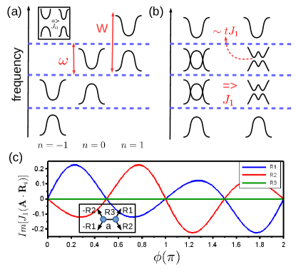
Figure 1: (color) (a) Floquet bands within first order emission/absorption photon processes as replicas of the original band structure modified by $J_{0}$ (see left upper inset). (b) formation of the Floquet band structure by merging states into single Brillouin zone (left) and accounting for the effect of gap opening due to $J_{1}$ (right). (c) The imaginary part of $J_{1}(\mathbf{A}\cdot\mathbf{R}_{j})$ as a function of polarization $\phi$ (in unit of $\pi$) when $\mathbf{A}=[1,7.467]/a$ (with $\hbar=e=1$). Left lower inset gives the definition of each $\mathbf{R}_{i}$ of graphene honeycomb lattice, where $a$ is the length of $\mathbf{R}_{3}$.

For the approximation (a), let us consider an ac–field sinusoidal in time. In this case, $J_{q}(\mathbf{A}\cdot\Delta\mathbf{r})$ is essentially the $q$–th Bessel function of the first kind. In the limit of the weak intensity, $|A|\rightarrow 0$, its asymptotic behavior is as follows: $J_{0}\rightarrow 1,$ $J_{q\neq 0}\rightarrow 0$. The larger the $q$ the faster $J_{q\neq 0}$ drops to zero. Hence we can truncate $H_{F}$ to a finite dimension by including just a few lowest order photon processes, provided the field intensity is weak enough. For example, if we keep $q=0,1$, $H_{F}$ is reduced to the following form

$$H_{F} \simeq\mathcal{P}_{1}H_{F}\mathcal{P}_{1}^{-1}=H_{f}^{1}=$$

$$\left(\begin{array}[]{ccc}h_{0}^{\alpha\beta}-1\omega I&h_{1}^{\alpha\beta}&0\\ h_{-1}^{\alpha\beta}&h_{0}^{\alpha\beta}&h_{1}^{\alpha\beta}\\ 0&h_{-1}^{\alpha\beta}&h_{0}^{\alpha\beta}+1\omega I\end{array}\right),$$

where $H_{f}^{1}$ denotes a reduced Floquet Hamiltonian describing an emission/absorbtion of a single photon and $\mathcal{P}_{1}$ is the operator that projects $H_{F}$ to $H_{f}^{1}$ . A diagrammatic explanation of such first order process is shown in Fig.1(a) and (b). In the upper left inset, the undriven band structure is modified by the 0–th order effect $J_{0}$. Once $J_{1}$ term comes in, the bands will have three copies with energy shifts $0,\pm\omega$. When those bands reach resonant energies, i.e the band crossings, $J_{1}$ will open gaps $\sim tJ_{1}$ making them anti–crossing. This is the main idea of the truncation. One has to note that when $H_{F}$ is truncated, the periodicity in frequency domain is broken, and the relations $\epsilon_{\gamma n}=\epsilon_{\gamma 0}+n\omega$ and $|u_{\gamma n}\rangle=|u_{\gamma 0}\rangle$ are strictly speaking no longer valid.

As for the approximation (b), let us assume the frequency of the external field is so much larger than the bandwidth, $\omega\gg W,$ that the Floquet bands do not cross anymore. In this limit, the gap openings due to $J_{q>0}$ become less important, which implies that it is also the condition to consider just the lowest order photon processes.

Time-Reversal Symmetry. In an undriven system, the TRS is defined by $\mathcal{T}H(\tau)\mathcal{T}^{-1}=H(-\tau)$ where $\mathcal{T}$ is the conventional TR operator $\mathcal{T}=e^{-i\pi\sigma_{y}/2}K$. Although systems with time–dependent ac–fields do not hold this property, it is still possible to define an effective TRS for the Floquet HamiltonianFTI-2 ; FB-2 . To give specific conditions holding the effective TRS, we conclude with two important theorems here (see Supplementary Materials):

Theorem I: If there exists a parameter $\tau_{0}$ such that $\mathcal{T}H(\tau)\mathcal{T}^{-1}=H(\tau+\tau_{0})$, one can always define an effective TR operator $Q=e^{iH_{F}\tau_{0}}\mathcal{T}$ that satisfies the relation $\mathcal{Q}H_{F}(\mathbf{k})\mathcal{Q}^{-1}=H_{F}(-\mathbf{k}).$

Theorem II: Assuming a system has TRS when it is undriven, i.e. $|\mathbf{A}|=0$, then $\mathbf{A}(\tau)=[A_{x}sin(\omega\tau+\phi_{x}),A_{y}sin(\omega\tau+\phi_{y}),A_{z}sin(\omega\tau+\phi_{z})]$ with $\phi_{i}-\phi_{j}=m\pi$ ($i,j\in\ x,y,z$; $m\in integers$) will automatically make $H(\tau)$ satisfy $\mathcal{T}H(\tau)\mathcal{T}^{-1}=H(\tau+\tau_{0})$. Furthermore if the time frame is properly chosen, one can always let all $\phi_{i}^{\prime}s=n_{i}\pi\ (n_{i}\in integer)$ such that $\tau_{0}=0$ and $Q=\mathcal{I}\mathcal{T}$

These theorems tell us if the phase differences among each field component are multiples of $\pi$, the Floquet Hamiltonian will have effective TRSFTI-6 and the TR operator can be treated as a conventional one acting in the Hilbert space of the basis of the Floquet Hamiltonian $\{|\alpha n(\mathbf{k})\rangle\}$. In the following, we will call the condition $\phi_{i}-\phi_{j}=m\pi$ as a linear polarization although the polarization is not definable if $\mathbf{A}$ is not in 2D.

The linear polarization condition is not the only option to have effective TRS. Since we are handling the $\nu$–th order reduced Floquet Hamiltonian $H_{f}^{\nu}$ rather than the original $H_{F}$ in a realistic calculation, it is possible that $H_{f}^{\nu}$ has more time–reversal points than $H_{F}$. Recall that the hopping integrals in the Floquet Hamiltonian are generated by modifying $t_{\alpha\beta}^{ij}\rightarrow t_{\alpha\beta}^{ij}J_{q}(\mathbf{A}(\tau)\cdot\Delta\mathbf{r})$. If one can properly tailor $\mathbf{A}$ such that $J_{q\leq\nu}$ are real numbers for all $\Delta\mathbf{r}$ in the lattice, obviously TRS will be kept up to $\nu$–th order $H_{f}^{\nu}$. Since $J_{0}$ is always real, the highest order $\nu$ should be equal or greater than 0. To give an example of $\nu>0$, we have plotted in Fig. 1(c) the imaginary part of $J_{1}$ with respect to three non–equivalent position vectors of a honeycomb lattice as a function of polarization $\phi=\phi_{x}-\phi_{y}$ by setting $[A_{x},A_{y}]=[1,7.467]/a$. One can immediately notice that there are two additional TRS points (all lines reach 0) other than $\phi=m\pi$, i.e. $\phi=\pi/2$ and $\phi=3\pi/2$. However, those TRS points are just results of low excitation approximation. One should always confirm that the energy splitting $\Delta E$ of Kramer degenerate states due to higher order terms is much smaller than the characteristic energy $\varepsilon_{c}$ that we are interested in ($\Delta E\sim tJ_{\nu+1}\ll\varepsilon_{c}$) to explore this feature further.

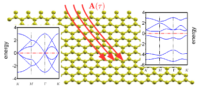
Figure 2: (color) Honeycomb lattice irradiated by electric ac-field $\mathbf{A}(\tau)$. Left inset: band structure without SOC. Right inset: band structure with SOC $\lambda=3t$,    $t$ being a unit of energy. Note that all the bands are doubly degenerate.

Floquet Topological Phases. The best candidates to realize the transition between a TRS Floquet $Z_{2}$ phase and a non–TRS Floquet Chern phase would be 2D materials with spin–orbit coupling, e.g transit–metal dichalcogenidesTMD-1 , graphene with adatomsGAD-1 ; GAD-2 , siliceneSIL-1 , germananeGER-1 , Tin filmsTIN-1 , $\alpha$-SnASN-1 , etc. These materials have been proven (or have high expectancy) to exhibit monolayer structures with band gaps around dozens to hundreds meV. Because of their planar geometry, the in–plane ac–field can be easily realized by a laser in experimental setup.

Here we consider a nearest neighbor tight–binding Hamiltonian on a honeycomb lattice with a $p$–orbital (total six states) per each site as a generic minimal model describing the 2D material at the center of interest. For simplicity, we assume the system is half–filled. In order to make our model close to actual band structures, hopping integrals are generated by a Slater–Koster methodSKI-1 with $V_{pp\sigma}=t$, $V_{pp\pi}=-t$ and onsite energy $E_{p_{x,y,z}}=0$. SOC is treated as a local potential by evaluating the matrix elements $\langle p_{i}|\lambda\mathbf{L}\cdot\mathbf{S}|p_{j}\rangle$ with $\lambda=3t$ for each site. In order to calculate the topological invariants, we implement the $n$–field method introduced Fukui et al.TII-1 . This method has been proven to provide evaluations of both $Z_{2}$ and Chern topological invariants in discretized Brillouin zones accurately and efficiently. We emphasize extra time that when computing $Z_{2}$ invariants for the Floquet Hamiltonian, the TR operator should be replaced by the effective TR operator $Q=e^{iH_{F}\tau_{0}}\mathcal{T}$  as described in this work.

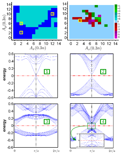
Figure 3: (color) Floquet topological phase diagram. Upper left: $Z_{2}$ phase diagram (green for $Z_{2}=0$ and blue for $Z_{2}=1$) with linearly polarized ac–field $[\phi_{x},\phi_{y}]=[0,0]$. Upper right: Chern phase diagram (Chern numbers for each color are shown in the legend) with eliptically polarized ac–field $[\phi_{x},\phi_{y}]=[0.0,0.5]\pi$. $A_{x}$ and $A_{y}$ are chosen to be $0.3n/a,\ n=1\sim 13$ ($a$ is lattice constant, $\hbar=e=1$). There are four points at the phase diagram labeled by $1\$to $4$ with their edge–state band structures shown (all energies in units of $t$) . Edge states are calculated in a zigzag ribbon geometry with $20$ sites in the transverse direction.

In Fig.2, we show a cartoon of the honeycomb lattice and the band structures with and without SOC. One can find that the Dirac points at high symmetry points $\Gamma$ and $K$ become gapped when SOC is turned on. This is a general feature of a system with the honeycomb lattice. To study the Floquet effect, we consider the reduced Floquet Hamiltonian to first order, $H_{f}^{1},$ and use a rather large frequency $\omega=10t$ (larger than the band width $\sim 8t$). The amplitudes of $A_{x}$ and $A_{y}$ are chosen to be $0.3n/a,\ n=1\sim 13$ ($a$ is the lattice constant) with linearly polarized field $\phi_{x}=\phi_{y}=0$. The Floquet bands are also assumed to be half–filled as in the undriven case. Fig.3 shows the $Z_{2}$ phase diagram and selected band structures (labeled by $1$ to $4$) of the edge states. Apparently there exists a large (shown in blue) area of $Z_{2}$ phase in the parameter space. To check the corresponding edge states, we have plotted the Floquet band structures of zigzag ribbons under the same ac–field. Plots corresponding to the parameters of phase points 1 and 3 are both $Z_{2}=1$ phases, so the Dirac cones appear in the gapped region as expected. An interesting finding for the phase point 3 is that the Dirac cone appears in $k=0$ rather than at $k=\pi/a$ as seen for the point 1. It is supposed to be the case of the armchair ribbon in the Kane-Mele model which now appears in the zigzag edge with appropriate parametersKMM-1 . It means the ac–field can not only tune the $Z_{2}$ topology from trivial to non–trivial, but also control the specific features of the edge states. Finally, we have also plotted the band structure corresponding to the trivial phase (point 2) as a confirmation that the edge Dirac cone indeed does not show up.

Now we discuss how to make the $Z_{2}$ phase transiting to a Chern phase. Let us consider an elliptically (circularly if $A_{x}=A_{{y}}$) polarized ac–field with $[\phi_{x},\phi_{y}]=[0,\pi/2]$. The phase diagram of the Chern numbers is shown in the upper right of Fig.3. Because it is a multiband problem (12 bands for the undriven and 36 bands for the reduced Floquet Hamiltonian), the Chern number can be much larger than $\pm 1$MTB-1 . We also show the edge states corresponding to the parameters of the phase point 4. The existence of two Dirac cones at the edge agrees with our $C=-2$ result very well. The phase diagrams of Fig.3 illustrate how $Z_{2}$ and Chern topological phases can be manipulated in a single material using properly tailored ac–fields.

Finally, we estimate some physical quantities relevant to realization of such exotic electronic phases in real systems. Let us take graphene with adatoms as an exampleGAD-1 . It is predicted to have SOC induced gap $E_{g}$ around $5\sim 20$ meV. To simulate this problem, we use tight–binding parameters for the $s\$and $p$ states of graphene obtained by fitting to its band structureGTB-1 and tune the SOC to a value that in our model fits the gap value of 5 meV. We consider two cases: a microwave field, $\omega=2GHz\ll E_{g}/\hbar,$ and an infrared field, $\omega=2THz\simeq E_{g}/\hbar$. Polarization angles are chosen to be $0$ and $\pi$ in order to observe $Z_{2}$ and Chern phases respectively. To ensure the weak intensity approximation, we limit $A_{x},A_{y}<1(\hbar/\mathring{A})$ for both cases so that $J_{2}$ effects are about two orders of magnitude smaller that $J_{1}$ and can be neglected. The electric field and the corresponding laser intensity are obtained by $E_{0}=A\omega/e$ and $I_{0}=\frac{1}{2}\epsilon_{0}cE_{0}^{2}=1.33\times 10^{-3}E_{0}^{2}(W/cm^{2})$ respectively. For the microwave case, we found that the Floquet $Z_{2}$ phase can be easily observed but the Chern phase cannot. This corresponds to the electric fields $E_{0}<131V/cm$ or the intensities $I_{0}<23W/cm^{2}$, which can be achieved by lasers with powers $P\lesssim 200mW$, easily accessible in experiment. As for the infrared case, we found both $Z_{2}$ and Chern phases can be generated within that regime. It corresponds to the electric fields $E_{0}<1.31\times 10^{5}V/cm$ or the intensities $I_{0}<2.3\times 10^{7}W/cm^{2}$. This will require a rather high power about several kW in experiments. This power is still experimentally accessible but most materials can burn out under such a strong field. Therefore searching for a material that can display both phases under lower intensities could be an interesting topic for future research. Although realization of $Z_{2}$–to–Chern phase transition could be difficult in experiments for our discussed system, we have to emphasize that easily achievable Floquet $Z_{2}$ phase still remains a treasure in problems of engineering topological electronic structures.

Conclusion. In summary, we have developed a framework to study TRS in Floquet Hamiltonian and used a generic tight–binding model of the honeycomb lattice relevant to several recently discovered monolyaered materials in order to demonstrate the transition between $Z_{2}$ and Chern phases by tuning the polarization of the ac–field. Although, our discussion is based on the dynamical analogies, the physics is still very fascinating not only due to the emergence of the $Z_{2}$ phase in a formally time–reversal breaking potential but also due to the possibility of manipulating self–contradictory topological phases in a single material. Both phenomena are hard to find in static systems but could lead us to a new physics that is unreachable in conventional solid–state matter.

Acknowledgments We would like to acknowledge the useful discussions with X. Dai, X. Wan, R. Wang and B. Wang. We also acknowledge the support by NSF DMR Grant No.1411336.

I Floquet Time-Reversal Symmetry

Define Floquet operator $u(T)$ and Floquet Hamiltonian $H_{F}$

$$u(T)=\mathbf{T}[e^{-i\int_{0}^{T}H(\tau)d\tau}]\equiv e^{-iH_{F}T}$$

where $T$ is the time periodicity of the Floquet system and $\mathbf{T}$ is the time-order product. We hope to find an effective time–reversal (TR) operator $\mathcal{Q}$ for the Flouqet operator and Floquet Hamiltonian such that

$$\mathcal{Q}u(T)\mathcal{Q}^{-1}=u(-T)$$

and

$$\mathcal{Q}H_{F}(\mathbf{k})\mathcal{Q}^{-1}=H_{F}(-\mathbf{k})$$

where $\mathcal{Q}$ is an antilinear oparator with $\mathcal{Q}^{2}=-1$. We claim that if there exists an parameter $\tau_{0}$ that satisfies the relation

$$\mathcal{T}H(\tau)\mathcal{T}^{-1}=H(-\tau+\tau_{0})$$

where $\mathcal{T}$ is the conventional TR operator. Then an effective $\mathcal{Q}$ can always be defined as

$$\mathcal{Q}\equiv u(0,\tau_{0})\mathcal{T}=e^{iH_{F}\tau_{0}}\mathcal{T}$$

In the following, we provide a proof for this theorem. (Note: Our proof is equivalent to the one shown in Ref.7 of the main article. Because we have chosen a slightly different statement, we prove it again here.)

Let us represent the conventional TR operator as the product of an unitary operator $\mathcal{S}$ (usually $e^{-i\pi\sigma_{y}/2}$) and the complex conjugate operator $\mathcal{K}$:

$$\mathcal{T}=\mathcal{S}\mathcal{K}$$

Assume there exists a parameter $\tau_{0}$ such that

$$\mathcal{T}H(\tau)\mathcal{T}^{-1}=H(-\tau+\tau_{0})\Longleftrightarrow\mathcal{S}H^{\ast}(\tau)\mathcal{S}^{\dagger}=H^{\dagger}(-\tau+\tau_{0})$$

Since

$$u(T,0) =\lim_{N\rightarrow\infty}e^{-i\Delta\tau H(T-\Delta\tau)}\times e^{-i\Delta\tau H(T-2\Delta\tau)}\times\cdots$$

$$\cdots\times e^{-i\Delta\tau H(0)}\ \ ;\ \ \Delta\tau=T/N$$

We have

$$\mathcal{S}u^{*}(T,0)\mathcal{S}^{\dagger} =\lim_{N\rightarrow\infty}e^{i\Delta\tau\mathcal{S}H^{*}(T-\Delta\tau)\mathcal{S}^{\dagger}}\times\cdots\times e^{i\Delta\tau\mathcal{S}H^{*}(0)\mathcal{S}^{\dagger}}$$

$$=\lim_{N\rightarrow\infty}e^{i\Delta\tau H^{\dagger}(\tau_{0}-T+\Delta\tau)}\times\cdots\times e^{i\Delta\tau H^{\dagger}(\tau_{0})}$$

$$=\lim_{N\rightarrow\infty}e^{i\Delta\tau H^{\dagger}(\tau_{0}+\Delta\tau)}\times\cdots\times e^{i\Delta\tau H^{\dagger}(\tau_{0}+T)}$$

$$=u^{\dagger}(\tau_{0}+T,\tau_{0})$$

where the third equal sign uses the relation $H(\tau+T)=H(\tau)$. Therefore if we define $\mathcal{R}\equiv u(0,\tau_{0})\mathcal{S}$ to shift the origin from $\tau_{0}$ to 0, then an effective TR operator can be defined as $\mathcal{Q}=\mathcal{R}\mathcal{K}$

$$\mathcal{R}u^{*}(T,0)\mathcal{R}^{\dagger} =u(0,\tau_{0})\mathcal{S}u^{*}(\tau,0)\mathcal{S}^{\dagger}u^{\dagger}(0,\tau_{0})$$

$$=u(0,\tau_{0})u^{\dagger}(\tau_{0}+T,\tau_{0})u^{\dagger}(0,\tau_{0})$$

$$=u^{\dagger}(T,0)$$

It means

$$\mathcal{Q}u(T,0)\mathcal{Q}^{-1}=u(-T,0)$$

and

$$\mathcal{Q}H_{F}(\mathbf{k})\mathcal{Q}^{-1}=H_{F}(-\mathbf{k})$$

II Relation to Polarization

Consider a vector potential $\mathbf{A}(\tau)=[A_{x}sin(\omega\tau+\phi_{x}),A_{y}sin(\omega\tau+\phi_{y}),A_{z}sin(\omega\tau+\phi_{z})]$. We claim two consequences:

• If $\phi_{i}-\phi_{j}=m\pi$ ($i,j\in x,y,z$, $m\in integer$), the Floquet time–reversal criterion: $\mathcal{T}H(\tau)\mathcal{T}^{-1}=H(-\tau+\tau_{0})$ will always be satisfied.

• If $\phi_{i}-\phi_{j}=m\pi$, one can always let $\phi_{i}=n_{i}\pi$ ($n_{i}\in integer)$ such that $\tau_{0}=0$ and the effective TR operator can be simply expressed as $\mathcal{Q}=\mathcal{IT}$.

The first theorem tells us the relation between the Floquet TR symmetry and the polarization of the ac–field. The second theorem helps us to deal with the effective TR operator in a much simpler way. In the following, we provide a proof for these two statements.

Consider the basis set of Hilbert space $\{|\alpha,\sigma\rangle\}$ where $\alpha$ is the label of space–related degree of freedom, e.g, sublattice, orbital, etc., and $\sigma=+/-$ is the spin index. Define time–reversal operator $\mathcal{T}=uK$ where $u=-i\sigma_{y}$. Then the matrix element of a time–reversal transformation applied to the Hamiltonian is given by

$$\langle\alpha\sigma|\mathcal{T}H\mathcal{T}^{-1}|\alpha^{{}^{\prime}}\sigma^{{}^{\prime}}\rangle =\langle\alpha\sigma|uH^{\ast}u^{\dagger}|\alpha^{{}^{\prime}}\sigma^{{}^{\prime}}\rangle$$

$$=(-1)^{[\delta_{\sigma-}+\delta_{\sigma^{{}^{\prime}}-}]}(H_{\alpha^{{}^{\prime}}-\sigma^{{}^{\prime}}}^{\alpha-\sigma})^{\ast}$$

If TR symmetry exists, $\mathcal{T}H\mathcal{T}^{-1}=H$, and we obtain a restriction on the matrix elements:

$$(-1)^{[\delta_{\sigma-}+\delta_{\sigma^{{}^{\prime}}-}]}(H_{\alpha^{{}^{\prime}}-\sigma^{{}^{\prime}}}^{\alpha-\sigma})^{\ast}=H_{\alpha^{{}^{\prime}}\sigma^{{}^{\prime}}}^{\alpha\sigma}$$

For a system with an ac–field, the hopping integral is modified by $t_{\alpha^{{}^{\prime}}\sigma^{{}^{\prime}}}^{\alpha\sigma}(\tau)\rightarrow t_{\alpha^{{}^{\prime}}\sigma^{{}^{\prime}}}^{\alpha\sigma}e^{i\mathbf{A}(\tau)(\mathbf{r}_{\alpha}-\mathbf{r}_{\alpha^{{}^{\prime}}})}$. The Floquet TR criterion $\mathcal{T}H(\tau)\mathcal{T}^{-1}=H(-\tau+\tau_{0})$ requires that

$$(-1)^{[\delta_{\sigma-}+\delta_{\sigma^{{}^{\prime}}-}]}(t_{\alpha^{{}^{\prime}}-\sigma^{{}^{\prime}}}^{\alpha-\sigma})^{\ast}e^{-i\mathbf{A}(\tau)(\mathbf{r}_{\alpha}-\mathbf{r}_{\alpha^{{}^{\prime}}})}$$

$$=t_{\alpha^{{}^{\prime}}\sigma^{{}^{\prime}}}^{\alpha\sigma}e^{i\mathbf{A}(-\tau+\tau_{0})(\mathbf{r}_{\alpha}-\mathbf{r}_{\alpha^{{}^{\prime}}})}$$

Assuming the system has TR symmetry when undriven, the hopping integrals will be canceled out and we have

$$-\mathbf{A}(\tau)=\mathbf{A}(-\tau+\tau_{0})$$ (2)

Because

$$\mathbf{A}(\tau)=[A_{x}sin(\omega\tau+\phi_{x}),A_{y}sin(\omega\tau+\phi_{y}),A_{z}sin(\omega\tau+\phi_{z})]$$

then Eq.2 means

$$-(\omega\tau+\phi_{i})+2n_{i}\pi=-\omega\tau+\omega\tau_{0}+\phi_{x}$$ (3)

$$\Rightarrow \ \phi_{i}=n_{i}\pi-\omega\tau_{0}/2,\ \ \ i\in x,y,z\ ;\ n_{i}\in integer$$

Since $\tau_{0}$ can be arbitrary real numbers, it is convenient to express the effective TR condition as

$$\phi_{i}-\phi_{j}=m\pi,\ \ \ m\in integer$$ (4)

For an in–plane ac–field, it is to say that a linearly polarized ac–field will have the Floquet TR symmetry. Furthermore, if Eq.4 is held, we can always choose $\tau_{0}=0$ and $\mathcal{Q}=\mathcal{IT}$. To show this, let us shift the time frame $\tau=\tau^{{}^{\prime}}+\tau_{0}/2$ and plug in the Eq.3. If so, we can get a new equation where $\phi_{i}=n_{i}\pi$ and $\tau_{0}^{{}^{\prime}}=0$.

References

- (1) M.Z. Hasan and C.L. Kane, Rev. Mod. Phys. 82, 3045 (2010)
- (2) B.A. Bernevig, T.L. Hughes and S.C. Zhang, Science 314, 1757 (2006); M. Konig, Science 318, 766 (2007); D. Hsieh et al., Nature 452, 970 (2007); Y. Xia et al., Nat. Phys. 5, 398 (2009); H. Zhang et al., Nat. Phys. 5, 438 (2009)
- (3) J.G. Checkelsky, J. Ye, Y. Onose , Y. Iwasa and Y. Tokur, Nat. Phys. 8, 729 (2012)
- (4) J. Liu, T.H. Hsieh, P. Wei, W. Duan, J. Moodera and L. Fu, Nat. Mater. 13, 178 (2014)
- (5) X. Qian, J. Liu, L. Fu, J. Li, Science 346, 1344 (2014)
- (6) M.S. Rudner, N.H. Lindned, E. Berg and M. Levin, Phys. Rev. X 3, 031005 (2013)
- (7) T. Kitagawa, E. Berg, M. Rudner, E. Demler, Phys. Rev. B 82, 235114 (2010)
- (8) T. Kitagawa, T. Oka, A. Brataas, L. Fu and E. Demler, Phys. Rev. B 84 235108 (2011)
- (9) N.H. Linder, D.L. Bergman, G. Refael and V. Galitski, Phys. Rev. B 87, 235131 (2013)
- (10) Y.T. Katan and D. Podolsky, Phys. Rev. Lett. 110, 016802 (2013)
- (11) J. Inoue, A. Tanaka, Phys. Rev. Lett. 105, 017401 (2010); T. Oka and H. Aoki, Phys. Rev. B 79, 081406 (2009); Z. Gu, H.A. Fertig, D.P. Arovas and A. Auerbach, Phys. Rev. Lett. 107, 216601 (2011)
- (12) N.H. Lindner , G. Refael and V. Galitski, Nat. Phys. 7, 490 (2011)
- (13) A. Kundu and B. Seradjeh, Phys. Rev. Lett. 111, 136402 (2013)
- (14) P. Delplace, A. Gomez-Leon and G. Platero, Phys. Rev. B 88, 245422 (2013)
- (15) A.G. Grushin, A. Gomez-Leon and T. Neupert, Phys. Rev. Lett. 112, 156801 (2014)
- (16) R. Wang, B. Wang, R. Shen, L. Sheng and D. Y. Xing, EPL 105 17004 (2014)
- (17) Y.H. Wang, H. Steinberg, P. Jarillo-Herrero. and N. Gedik, Science 342, 453 (2013)
- (18) M.C. Rechtsman et. al., Nature 496, 196 (2013)
- (19) C. Weeks, J. Hu, J. Alicea, M. Franz and R. Wu, Phys. Rev. X 1, 021001 (2011)
- (20) J. Hu, J. Alicea, R. Wu and M. Franz, Phys. Rev. Lett. 109, 266801 (2012)
- (21) Z. Gong, G.-B. Liu, H. Yu, D. Xiao, X. Cui, X. Xu and W. Yao, Nat. Comm. 4, 2053 (2013); X Xu, W. Yao, D. Xiao and T.F. Heinz, Nat. Phys. 10, 343 (2014)
- (22) B. Lalmi et al., Appl. Phys. Lett. 97, 223109 (2010); P. Vogt et al., Phys. Rev. Lett. 108, 155501 (2012)
- (23) E. Bianco et al., ACS Nano. 7, 4414 (2013); S. Jiang et al., Nat. Comms. 5, 3389 (2014)
- (24) Y. Xu et al., Phys. Rev. Lett. 111, 136804 (2013); B.-H. Chou et al., New J. Phys. 16 115008 (2014)
- (25) A. Barfuss et. al., Phys. Rev. Lett. 111, 157205 (2013); Y. Ohtsubo et al., Phys. Rev. Lett. 111, 216401 (2013); T. Eguchi et al., J. Phys. Soc. Jap. 67, 381 (1998)
- (26) J.C. Slater and G.F. Koster, Phys. Rev. 94, 1498 (1954)
- (27) T. Fukui, Y. Hatsugai and H. Suzuki, J. Phys. Soc. Jap. 74, 1674 (2005); T. Fukui and Y. Hatsugai, J. Phys. Soc. Jap. 76, 053702 (2007)
- (28) C.L. Kane and E.J. Mele, Phys. Rev. Lett. 95, 146802 (2005); C.L. Kane and E.J. Mele, Phys. Rev. Lett. 95, 226801 (2005)
- (29) A. Masao and Y. Hatsugai, J. Phys.: Conf. Ser. 334 012042 (2011)
- (30) R. Saito, M. Fujuta, G. Dresselhaus and M.S. Dresselhaus, Phys. Rev. B 46, 1804 (1992); H. Min et. al., Phys. Rev. B 74, 165310 (2006)