Fermions in the background of mixed vector-scalar-pseudoscalar square potentials

Abstract

The general Dirac equation in 1+1 dimensions with a potential with a completely general Lorentz structure is studied. Considering mixed vector-scalar-pseudoscalar square potentials, the states of relativistic fermions are investigated. This relativistic problem can be mapped into a effective Schrödinger equation for a square potential with repulsive and attractive delta-functions situated at the borders. An oscillatory transmission coefficient is found and resonant state energies are obtained. In a special case, the same bound energy spectrum for spinless particles is obtained, confirming the predictions of literature. We showed that existence of bound-state solutions are conditioned by the intensity of the pseudoscalar potential, which posses a critical value.

1 Introduction

Since its formulation in 1928 [1], the Dirac equation has been widely investigated in various physical systems. Among the applications, we can highlight the Klein’s paradox [2, 3, 4], the description of electrons in graphene [5], the influence of the nuclear medium on the nucleons [6] and the relativistic hydrogen atom [7].

The pseudospin symmetry (PSS) is a topic of intense discussion, activities and recent progress in the last decades. PSS was introduced in nuclear physics for explain the degeneracies of orbitals in single particle spectra [8, 9]. In order to understand the origin of PSS, we need to take into account the motion of the nucleons in a relativistic mean field and thus consider the Dirac equation [10, 11, 12]. The case in which the mean field is composed by a vector ($V_{t}$) and a scalar ($V_{s}$) potential, with $\Sigma=V_{t}+V_{s}=0$ ($V_{t}=-V_{s}$) is usually pointed out as a necessary condition for occurrence of PSS in nuclei [10, 11, 12]. The study of symmetries in resonant states is certainly an interesting topic. The authors of Ref. [13] showed that the PSS in single particle resonant states in nuclei is exactly conserved, i.e., the pseudospin doublets with different quantum numbers $\kappa$ e $-\kappa+1$ have the same resonant state with energy $E_{\mathrm{res}}$ and width $\Gamma_{\mathrm{res}}$. That novel result were illustrated for single particle resonances in spherical square-well and Woods–Saxon potentials. Additionally, the Dirac equation exhibit spin symmetry (SS) when the vector and scalar potentials have the same magnitude and was used for explain the small spin-orbit splitting in hadrons [14]. Recently, a comprehensive review of the progress on the PSS and SS in various systems and potentials have been reported in [15], including extensions of the PSS study from stable to exotic nuclei, from non-confining to confining potentials, from local to non-local potentials, from central to tensor potentials, from bound to resonant states, from nucleon to anti-nucleon spectra, from nucleon to hyperon spectra, and from spherical to deformed nuclei.

The four-dimensional Dirac equation with a mixture of spherically symmetric scalar, vector and tensor interactions can be reduced to the two-dimensional Dirac equation with a mixture of scalar, vector and pseudoscalar couplings when the fermion is limited to move in just one direction ($p_{y}=p_{z}=0$) [16]. In this restricted motion the scalar and vector interactions preserve their Lorentz structures, while the tensor interaction becomes a pseudoscalar. This kind of dimensional reduction is very useful because the two-dimensional version of the Dirac equation can be thought as that one describing a fermion embedded in a four-dimensional space-time with either spin up or spin down [7]. Furthermore, the absence of angular momentum and spin-orbit interaction as well as the use of $2\times 2$ matrices, instead of $4\times 4$ matrices, allow us to explore the physical consequences of the negative-energy states in a mathematically simpler and more physically transparent way. Therefore, we can take advantage of the simplicity of the lowest dimensionality of the space-time.

Considering mixed scalar-vector potentials the Dirac equation in (1+1) dimensions have been investigated for a sign potential [17] and smooth step potential [18]. In the context of mixed scalar-vector-pseudoscalar potentials (the most general Lorentz structure), the bound-state solutions for fermions and antifermions in (1+1) dimensions have been studied for harmonic oscillator potential [19], Pöschl-Teller potential [20], Cornell potential [21, 22] and Coulomb potential [23]. In those works, the relation between spin and pseudospin symmetries using charge-conjugation and chiral transformation was illustrated.

The square potentials, wells and barriers, are models widely used in low-dimensional systems such as the quantum dots [24], Dirac fermions in graphene [25], electrons in semiconductor heterostructures [26] and theoretical studies [27, 28]. Besides these applications, the well and barrier potentials are extremely examples used as toy-models in textbooks (for example, see [7] ), further increasing its importance in quantum mechanics.

The main motivation of this paper is the approach of the Dirac equation (1+1) dimensional in the framework of mixed vector-scalar-pseudoscalar square potentials. The scattering solutions furnish an oscillatory transmission coefficient, which does not present a total reflection. The presence of bound-state solutions are conditioned by the intensity of the pseudoscalar potential, which possess a critical value, compared to the mixed vector-scalar potential. Those interesting results are obtained as solutions of an effective Schrödinger equation for a square potential with repulsive and attractive delta-functions situated at the borders. The results can give us support for study PSS and SS in high dimensionality of the space-time.

2 The Dirac equation in (1+1) D

The time-independent Dirac equation for a fermion of rest mass $m$ in the background of vector ($V_{t}$), scalar ($V_{s}$) and pseudoscalar ($V_{p}$) potentials can written as (with units in which $\hbar=c=1$ )

$$H\psi=E\psi,\quad H=\sigma_{1}p+\sigma_{3}m+\frac{1+\sigma_{3}}{2}\Sigma+\frac{1-\sigma_{3}}{2}\Delta+\sigma_{2}V_{p}$$ (1)

where $\sigma_{1},\sigma_{2}$ and $\sigma_{3}$ are the Pauli matrices and $\Sigma=V_{t}+V_{s},$ $\Delta=V_{t}-V_{s}.$

The Dirac equation is covariant under $x\rightarrow-x$ if  $V_{p}$ changes sign whereas $V_{s}$ and $V_{t}$ remain the same. This is because the parity operator $P=\exp\left(i\varepsilon\right)P_{0}\sigma_{3}$, where $\varepsilon$ is a constant phase and $P_{0}$ changes $x$ into $-x$, changes the sign of $\sigma_{1}$ and $\sigma_{2}$ but not of $\sigma_{3}$.

The charge-conjugation operation is accomplished by the transformation $\psi_{c}=\sigma_{1}\psi^{\ast}$ and the Dirac equation becomes $H_{c}\psi_{c}=-E\psi_{c}$, with

$$H_{c}=\sigma_{1}p+\sigma_{3}m-\frac{I+\sigma_{3}}{2}\,\Delta-\frac{I-\sigma_{3}}{2}\,\Sigma+\sigma_{2}V_{p}\,.$$ (2)

One see that the charge-conjugation operation changes the sign of the energy and of the potentials $V_{t}$ and $V_{p}$. In turn, this means that $\Sigma$ turns into $-\Delta$ and $\Delta$ into $-\Sigma$. Therefore, to be invariant under charge conjugation, the Hamiltonian must contain only a scalar potential.

The chiral operator for a Dirac spinor is the matrix $\gamma^{5}=\sigma_{1}$. Under the discrete chiral transformation the spinor is transformed as $\psi_{\chi}=\gamma^{5}\psi$ and the transformed Hamiltonian $H_{\chi}=\gamma^{5}H\gamma^{5}$ is

$$H_{\chi}=\sigma_{1}p-\sigma_{3}m+\frac{I+\sigma_{3}}{2}\,\Delta+\frac{I-\sigma_{3}}{2}\,\Sigma+\sigma_{2}V_{p}.$$ (3)

This means that the chiral transformation changes the sign of the mass and of the scalar and pseudoscalar potentials, thus turning $\Sigma$ into $\Delta$ and vice versa. A chiral invariant Hamiltonian needs to have zero mass and $V_{s}$ and $V_{p}$ zero everywhere.

The equation (1) decomposes into two first-order equations for the upper, $\psi_{+},$ and the lower, $\psi_{-},$ components of the spinor:

$$-i\frac{d\psi_{-}}{dx}+m\psi_{+}+\Sigma(x)\psi_{+}-iV_{p}\psi_{-}=E\psi_{+}$$ (4)

$$-i\frac{d\psi_{+}}{dx}-m\psi_{-}+\Delta(x)\psi_{-}+iV_{p}\psi_{+}=E\psi_{-}$$ (5)

The components of four-current are given by $J^{0}=\psi^{\dagger}\psi$ and $J^{1}=\psi^{\dagger}\sigma_{1}\psi$. If we use the spinor $\psi$ in terms of its components the four-current is expressed by $J^{0}=$ $|\psi_{+}|^{2}+|\psi_{-}|^{2}$ and $J^{1}=2\mathrm{Re}(\psi_{+}^{\ast}\psi_{-})$ which are conserved quantities for stationary states. Then, the Dirac spinor is normalized as $\int_{-\infty}^{+\infty}dxJ^{0}=1$, so that $\psi_{+}$ and $\psi_{-}$ are square integrable functions. It is clear from the pair of coupled first-order differential equations (4) and (5) that $\psi_{+}$ and $\psi_{-}$ have opposite parities if the Dirac equation is covariant under $x\rightarrow-x$.

For $\Delta=0$ and $E\neq-m$, using the expression for $\psi_{-}$ obtained from (5) and inserting it into eq. (4) the Dirac equation for $\psi_{+}$ becomes

$$\psi_{-}=-\frac{i}{E+m}\left(\frac{d\psi_{+}}{dx}-V_{p}\psi_{+}\right)$$ (6)

$$-\frac{d^{2}\psi_{+}}{dx^{2}}+\left[(E+m)\Sigma+V_{p}^{2}+\frac{dV_{p}}{dx}\right]\psi_{+}=\left(E^{2}-m^{2}\right)\psi_{+}$$ (7)

Therefore, the solution of the relativistic problem is mapped into a Sturm-Liouville problem for the upper component of the Dirac spinor. As discussed in the ref. [20], we can take advantage of the discrete chiral transformation ($\gamma^{5}$) and we can obtain the solutions for $\Sigma=0$ from the $\Delta=0$ case. This means that the chiral symmetry is invoked to obtain the equations obeyed by $\psi_{+}$ and $\psi_{-}$, for $\Sigma=0$ and $E\neq m$. They are obtained from the previous ones by doing $\psi_{+}\leftrightarrow\psi_{-}$, $m\rightarrow-m$, $\Sigma\rightarrow\Delta$ and $V_{p}\rightarrow-V_{p}$ . The solutions for $\Delta=0$ with $E=-m$ and $\Sigma=0$ with $E=m$, called isolated solutions [29, 30, 22], are obtained directly from the original first-order equations (4) and (5). For $\Delta=0$ and $E=-m$, we obtain

$$\frac{d\psi_{+}}{dx}-V_{p}\psi_{+}=0$$ (8)

$$\frac{d\psi_{-}}{dx}+V_{p}\psi_{-}=-i\left(\Sigma+2m\right)\psi_{+}$$ (9)

whose solution is

$$\psi_{+}=N_{+}\mathrm{e}^{+v(x)}$$ (10)

$$\psi_{-}=\left[N_{-}-iN_{+}I(x)\right]\mathrm{e}^{-v(x)}$$ (11)

where $N_{+}$ and $N_{-}$ are normalization constants, and

$$v(x)=\int^{x}dyV_{p}(y)$$ (12)

$$I(x)=\int^{x}dy\left[\Sigma(y)+2m\right]\mathrm{e}^{+2v(y)}.$$ (13)

Note that this sort of isolated solution cannot describe scattering states and inasmuch as $\psi_{+}$ and $\psi_{-}$ are normalizable functions, the possible isolated solution implies that $V_{p}\neq 0$, therefore the presence of a pseudoscalar potential is sine qua non for provide isolated solutions [22].

3 The Square Potentials

Lets us consider

$$\Sigma(x)=C_{\Sigma}g(x)\,,$$ (14)

$$\Delta=0\,,$$ (15)

$$V_{p}(x)=C_{p}g(x)$$ (16)

$$g(x)=\frac{1}{2}\left[\mathrm{sgn}(x-a)-\mathrm{sgn}(x+a)\right]$$ (17)

where $\mathrm{sgn}(x)=x/|x|$ ($x\neq 0$) is the sign function, $C_{\Sigma}$ and $C_{p}$ are constants with dimensions of energy. Due to the chiral symmetry we can focus the discussion on the $\Sigma$ case ($\Delta=0$). The results for the case $\Delta\neq 0,$ $\Sigma=0$ and $V_{p},$ still given by (16), can be easily obtained by just changing the signs of $m$ and $C_{p}$ in the relevant expressions.

For the potentials (14), (15) and (16) we have not found a normalizable isolated solution with $E=-m$, i.e., the absence of isolated solution is because $V_{p}(x)=0$ for $|x|>a$ and therefore $\psi_{+}$ is a constant. For the case $E\neq-m$ the Eq. (7) takes the form

$$-\frac{d^{2}\psi_{+}}{dx^{2}}+V_{\mathrm{eff}}(x)\psi_{+}=k^{2}\psi_{+}$$ (18)

where

$$V_{\mathrm{eff}}(x)=\left[C_{\Sigma}(E+m)-C_{p}^{2}\right]g(x)+\frac{C_{p}}{2}\left[\delta(x-a)-\delta(x+a)\right],$$ (19)

$\delta(x)$ is the Dirac delta function and the effective energy particle is given by $k^{2}/2m$, with $k^{2}=E^{2}-m^{2}$. We note that the effective potential distinguishes particles and anti-particles if $C_{\Sigma}\neq 0$, and so we can not expect a symmetric spectrum with respect to $E$.

Let us introduce the parameter $r\equiv V_{\text{eff}}(\left|x\right|<a)$, where

$$V_{\text{eff}}(\left|x\right|<a)=C_{p}^{2}-C_{\Sigma}(E+m)\,.$$ (20)

The parameter $r$ characterizes three different profiles for the effective potential as illustrated in figure ( 1). If $r<0$, the effective potential consists in a finite square well potential at the region $-a<x<+a$ with attractive and repulsive delta function situated at $x=-a$ and $x=+a$, respectively. If $r=0$, the effective potential consists in a double delta function potential with attractive and repulsive delta function situated at $x=-a$ and $x=+a$, respectively. Finally, if $r>0$, the effective potential consists in a finite square barrier potential at the region $-a<x<+a$ with attractive and repulsive delta function situated at $x=-a$ and $x=+a$, respectively.

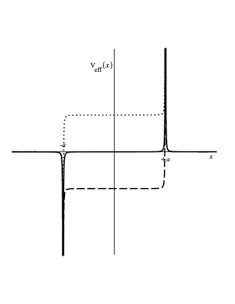
Figure 1: Profiles for effective potential $V_{\mathrm{eff}}(x)$ for $r>0$ (pointed line), $r=0$ (thin line) and $r<0$ (dashed line).

3.1 Scattering States

We focused our attention to the scattering states solutions that describes a fermion moving from left to right. In this way, $\psi(x\rightarrow-\infty)$ describes an incident wave moving to the right and a reflected wave moving to the left, and $\psi(x\rightarrow-\infty)$ describes a transmitted wave moving to the right or an evanescent wave. The upper components for scattering states are written as

$$\psi_{+}(x)=\left\{\begin{tabular}[]{cc}$A_{+}\exp(ikx)+A_{-}\exp(-ikx)$&for $x<-a$\\ $B_{+}\exp(i\eta x)+B_{-}\exp(-i\eta x)$&for $\left|x\right|<a$\\ $D_{\pm}\exp(ikx)$&for $x>+a$\end{tabular}\right.$$ (21)

where

$$\eta=\sqrt{k^{2}-r}\text{ \ \ }$$ (22)

The group velocity of the waves described above is given by

$$v_{g}=\frac{dE}{dk}=\pm\frac{k}{\sqrt{k^{2}+m^{2}}}$$ (23)

where the double signal is related to propagation direction. For both range the probability current densities are given by

$$J^{1}(x\rightarrow-\infty)=\frac{2k}{E+m}(\left|A_{\pm}\right|^{2}-\left|A_{\mp}\right|^{2})\text{ \ \ \ \ \ \ for \ \ \ \ \ \ }E\gtrless-m$$ (24)

and

$$J^{1}(x\rightarrow+\infty)=\pm\frac{2k}{E+m}\left|D_{\pm}\right|^{2}\text{ \ \ \ for \ \ \ \ \ \ }E\gtrless-m$$ (25)

Note that $J^{1}(-\infty)=J_{inc}-J_{ref}$ and $J^{1}(+\infty)=J_{trans}$, where $J_{inc}$, $J_{ref}$ and $J_{trans}$ are nonnegative quantities characterizing the incident, reflected and transmitted waves, respectively. If $E+m>0$, then $A_{+}e^{+ikx}$ ($A_{-}e^{-ikx}$) will describe the incident (reflected) wave, and $D_{-}=0$. On the other hand, if $E+m<0$, then $A_{-}e^{-ikx}$ ($A_{+}e^{+ikx}$) will describe the incident (reflected) wave, and $D_{+}=0$.

To determinate the reflection and transmission coefficients, we use the probability current densities given by (24) and (25). The $x$-independent probability current allow us to define the reflection and transmission coefficients as

$$R_{\pm}=\left|r_{\pm}\right|^{2}\text{ \ ,\ \ }T_{\pm}=\left|t_{\pm}\right|^{2}\text{ \ \ \ with \ \ \ \ }R_{\pm}+T_{\pm}=1$$ (26)

where the quantities

$$r_{\pm}=\frac{A_{\mp}}{A_{\pm}}\text{ \ \ \ \ \ \ and \ \ \ }t_{\pm}=\frac{D_{\pm}}{A_{\pm}}$$ (27)

are called reflection and transmission amplitudes, respectively.

We demand that $\psi_{+}$ be continuous at $x=\pm a$, that is

$$\lim_{\sigma\rightarrow 0}\psi_{+}(x)\mid_{x=\pm a-\sigma}^{x=\pm a+\sigma}=0\,.$$ (28)

Moreover, the effect due to the delta function potential on $d\psi_{+}/dx$ in the neighborhood of $x=\pm a$ can be evaluated by integrating (18) from $\pm a-\sigma$ to $\pm a+\sigma$ and taking the limit $\sigma\rightarrow 0$. Thereby, we obtain

$$\lim_{\sigma\rightarrow 0}\frac{d\psi_{+}(x)}{dx}\mid_{x=\pm a-\sigma}^{x=\pm a+\sigma}=\pm\frac{C_{p}}{2}\psi_{+}(x=\pm a)\,.$$ (29)

With $\psi_{+}(x)$ given by (21), conditions (28) and (29) imply that

$$B_{+}e^{-i\eta a}+B_{-}e^{i\eta a}=A_{+}e^{-ika}+A_{-}e^{ika}$$ (30)

$$D_{\pm}e^{ika}=B_{+}e^{i\eta a}+B_{-}e^{-i\eta a}$$ (31)

$$ikD_{\pm}e^{ika}-i\eta\left(B_{+}e^{i\eta a}-B_{-}e^{-i\eta a}\right)=\frac{C_{p}}{2}\left(B_{+}e^{i\eta a}+B_{-}e^{-i\eta a}\right)$$ (32)

$$\begin{split}i\eta\left(B_{+}e^{-i\eta a}-B_{-}e^{i\eta a}\right)-&ik\left(A_{+}e^{-ika}-A_{-}e^{ika}\right)=\\ &-\frac{C_{p}}{2}\left(B_{+}e^{-i\eta a}+B_{-}e^{i\eta a}\right)\end{split}$$ (33)

Omiting the algebraic details, we obtain the relative amplitudes

$$\frac{B_{+}}{A_{\pm}}=\frac{i\eta k\left(\eta+k+iC_{p}/2\right)e^{-i(k+\eta)a}}{2d}$$ (34)

$$\frac{B_{-}}{A_{\pm}}=\frac{k^{2}\eta\left(\eta-k-iC_{p}/2\right)e^{i(\eta-k)a}}{2d}$$ (35)

$$\frac{A_{\mp}}{A_{\pm}}=\frac{i\eta k\left[\eta^{2}-\left(k+iC_{p}/2\right)^{2}\right]\sin(4\eta a)e^{-2ika}}{2d}$$ (36)

$$\frac{D_{\pm}}{A_{\pm}}=\frac{e^{-2ika}}{d}$$ (37)

where

$$d\equiv\cos(2\eta a)-\sin(2\eta a)f(k)$$ (38)

and

$$f(k)\equiv i\frac{k^{2}+C_{p}^{2}/4+\eta^{2}}{2\eta k}\,.$$ (39)

The equation (37) given us the transmission coefficient

$$T=\frac{1}{1+\sin^{2}(2\eta a)\left[\left|f(k)\right|^{2}-1\right]-2\sin(4\eta a)\mathrm{\mathrm{Re}}\left[f(k)\right]}\,.$$ (40)

The scattering process is only possible with localized energies in the range $\left|E\right|>m$ and then $k$ $\in$ $\mathbb{R}.$ We see that both the effective potential as the transmission coefficient depends on the energy and then the transmission coefficient is not symmetric with respect to $E$. We can see that the transmission increases with energy, namely, $\left|E\right|\rightarrow\infty$ $T\rightarrow 1.$ The transmission coefficient provides us the necessary condition to obtain the resonant states

$$\eta=\frac{\left(N+1\right)\pi}{2a},\text{ \ \ \ \ where \ }N=0,1,2,3..$$ (41)

Therefore, the energies of resonant states can be writen as

$$E=\pm\sqrt{\frac{\left(N+1\right)^{2}\pi^{2}}{4a^{2}}+\left(m-C_{\Sigma}\right)^{2}+\frac{C_{p}^{2}}{4}}-C_{\Sigma}$$ (42)

and in the limit $N\rightarrow\infty$, we obtain

$$E=\pm\frac{N\pi}{2a}\,.$$ (43)

For this case $r=0$ the energy is fixed ($E=C_{p}^{2}/C_{\Sigma}-m$) and we can see that the pseudoscalar potential influence to transmission coefficient as showed in figure 2. From figure 2, we note an oscillatory behavior and no full reflection, as expected. As $T$ does not depend on the sing of $C_{p}$ the transmission coefficient have the same values from both barrier and well pseudoscalar potentials.

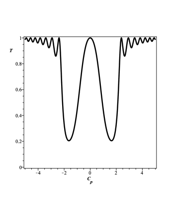
Figure 2: Transmission coefficient for $r=0$, $C_{\Sigma}=2$, $m=a=1$.

Some profiles for transmission coefficient are show in the figure 3 for differents values of $C_{p}$ and $C_{\Sigma}$. We can see that there is not full reflection for all cases. Further, from figure 3 we can note that curves of the transmission coefficient for negative energy are closer between them in comparasion to curves for positive energy. As expected, for very high energy, $T\rightarrow 1$ and also observe that the pseudoscalar potential maintains the oscillatory behavior of $T$.

Also, we can observe that the energies from resonant states is much similar to bound state energies for an infinity double-step potential

$$V_{p,\Sigma}(x)=\left\{\begin{tabular}[]{ccc}$-\infty$&&$x<-a$\\ $C_{p,\Sigma}$&&$x\leq|a|$\\ $+\infty$&&$x>a$\end{tabular}\right.$$ (44)

in the limit $N\rightarrow\infty$

$$E=\pm\sqrt{\frac{\left(N+1\right)^{2}\pi^{2}}{4a^{2}}+\left(m+\frac{C_{\Sigma}}{2}\right)^{2}+C_{p}^{2}}+\frac{C_{\Sigma}}{2}.$$ (45)

The similarity is because the bound state energies corresponds approximately to real part of the resonant energies obtained from the poles of the transmission amplitude for a square well [31]. A study on correspondence between behavior of $T$ and the bound-state energies for nonrelativistic square wells and barriers was done by Maheswari and collaborators [32]. But the authors make some mistakes, corrected by Ahmed [33], which also discusses some criteria to find oscillatory $T$ for a potential class.

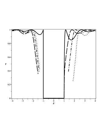
Figure 3: Transmission coefficient for $m=a=1$; $C_{p}=0$, $C_{\Sigma}=1$ (solid line); $C_{p}=1$, $C_{\Sigma}=0$ (solid-dot line); $C_{p}=1$, $C_{\Sigma}=0.5$ (long dashed line); $C_{p}=1$, $C_{\Sigma}=-0.5$ (pointed line).

3.2 Bound States

The bound-states solutions ($\left|E\right|<m$) can be obtained from (21) using the prescription $k=+i\left|k\right|$ and $A_{+}=D_{-}=0$ or $k=-i\left|k\right|$ and $A_{-}=D_{+}=0,$ i.e., the bound-states solutions correspond to the poles of the transmission amplitude. The conditions (28) and (29) providing the following quantization condition

$$\frac{2\eta\left|k\right|}{\eta^{2}+C_{p}^{2}/4-\left|k\right|^{2}}=\tan(2\eta a)$$ (46)

We note that the above condition does not depend on the sign of $C_{p}$ (barrier or square well pseudoscalar potential), and hence the energies does not depend on the localization of the delta function. Using the trigonometric relation $\cot(\theta)=-\tan(\theta/2)\pm\sqrt{1+\cot^{2}(\theta)}$, the quantization condition can be rewrite as

$$\tan(\eta a)=\pm\sqrt{1+\left[f(k)\right]^{2}}-f(k)$$ (47)

We can see that in the absence of pseudoscalar potential ($C_{p}=0$), the quantization condition is the same obtained for spin-$0$ bosons [34]. This equivalence confirm the results obtained by P. Alberto and collaborators [35], which show that the spin and pseudospin symmetries in Dirac equation produce an equivalent energy espectra for relativistic spin-$1/2$ and spin-$0$ particles in the presence of vector and scalar potentials.

3.2.1 Case $r\geq 0$.

For $r=0$ we have $\eta=\pm i\left|k\right|$, therefore (46) can be writen as

$$\frac{2\left|k\right|^{2}}{C_{p}^{2}/4-2\left|k\right|^{2}}=\tanh(2\left|k\right|a).$$ (48)

The above condition has just one solution in $\left|k\right|=0,$ therefore we do not have bound-states solutions for $r=0$. The case $r>0$ has a repulsive barrier between the two delta functions, and does not contain bound-states solutions too. The equation (20) and the condition $\left|E\right|<m$ allows us to conclude that only have bound states for $C_{\Sigma}>0$.

3.2.2 Case $r<0$.

For $r<0$ we have the condition $0\leq C_{p}^{2}<2mC_{\Sigma}$ and the quantization conditions provides the figures 4 and 5.

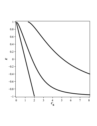
Figure 4: Bound-states espectrum for $C_{p}=0$, $m=a=1$.

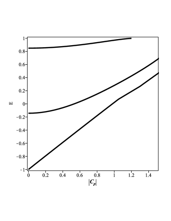
Figure 5: Bound-states espectrum for $C_{\Sigma}=2$, $m=a=1$.

The effective potential given by equation (19) has not defined parity, and therefore do not know the parity of the solutions. Obviously, the case $C_{p}=0$ show energy levels with parity defined, even (odd) solutions to negative (positive) sign in (47), the same behavior is found in reference [34]. The ground state energy ($E_{g.s}$), in the figure 4 (5), is given by $E_{g.s}\simeq m-C_{\Sigma}$ ($E_{g.s}\simeq m-C_{p}\mathrm{sgn}(C_{p})$). Therefore we obtain the constrain $C_{\Sigma}+C_{p}\mathrm{sgn}(C_{p})=2m$ for the low-energy state. As we already know, there are always bound-states solutions (at least one) if the intensity of the pseudoscalar barrier or well not exceeds the critical value $C_{p}^{critic}=\sqrt{2mC_{\Sigma}}$, for $C_{\Sigma}\neq 0$.

4 Conclusions

The states of fermions in the framework of mixed vector-scalar-pseudoscalar square potentials was investigated. The condition for spin symmetry ($\Delta=0$) enables to decouple the Dirac equation in an effective Schrödinger equation with a square potential with repulsive and attractive delta-functions situated at the borders for the upper component; and the lower component was expressed in term of the upper component in a simple way. An oscillatory transmission coefficient and resonant states energy were obtained. We showed that existence of bound-state solutions are conditioned by the intensity of the pseudoscalar potential, which posses a critical value $C_{p}^{critic}=\sqrt{2mC_{\Sigma}}$ for $C_{\Sigma}\neq 0$. In the absence of pseudoscalar potential, we obtain the same spectrum for spinless particles [34], confirming the predictions of Ref. [35].

This work can illustrate some general conclusions drawn in previous works about spin and pseudospin symmetries, we can obtain the solutions for $\Sigma=0$ from the $\Delta=0$ case, using the chiral transformation (changing the signs of $m$ and $C_{p}$ in the relevant expressions). Finally, it is well known that square potentials, wells and barriers are of certain interest in solid state physics, therefore our results could be applied to refine one-dimensional potential models caused by ions in a periodic crystal lattice, as the Kronig–Penney model [36]. Other possible application of our results could be in the neutron scattering on nucleus, where bound-state informations are extract for many isotopes in well [37].

References

- Dirac [1928] P. A. M. Dirac, Proc. R. Soc. Lon. A 117 (1928) 610.
- Klein [1929] O. Klein, Z. Phys. 53 (1929) 157.
- Su et al. [1993] R.-K. Su, G. G. Siu, X. Chou, J. Phys. A: Math. Gen. 26 (1993) 1001.
- Calogeracos and Dombey [1999] A. Calogeracos, N. Dombey, Int. J. Mod. Phys. A 14 (1999) 631.
- Castro Neto et al. [2009] A. H. Castro Neto, F. Guinea, N. M. R. Peres, K. S. Novoselov, A. K. Geim, Rev. Mod. Phys. 81 (2009) 109.
- Serot and Walecka [1986] B. D. Serot, J. D. Walecka, Advances in nuclear physics, volume 16, Plenum, New York, 1986.
- Greiner [1990] W. Greiner, Relativistic Quantum Mechanics: Wave Equations, Springer, Berlin, 1990.
- Arima et al. [1969] A. Arima, M. Harvey, K. Shimizu, Phys. Lett. B 30 (1969) 517.
- Hecht and Adler [1969] K. Hecht, A. Adler, Nucl. Phys. A 137 (1969) 129.
- Ginocchio [1997] J. N. Ginocchio, Phys. Rev. Lett. 78 (1997) 436.
- Ginocchio [1999] J. N. Ginocchio, Phys. Rep. 315 (1999) 231.
- Ginocchio [2005] J. N. Ginocchio, Phys. Rep. 414 (2005) 165.
- Lu et al. [2012] B.-N. Lu, E.-G. Zhao, S.-G. Zhou, Phys. Rev. Lett. 109 (2012) 072501.
- Page et al. [2001] P. R. Page, T. Goldman, J. N. Ginocchio, Phys. Rev. Lett. 86 (2001) 204.
- Liang et al. [2015] H. Liang, J. Meng, S.-G. Zhou, Phys. Rep. 570 (2015) 1.
- Strange [1998] P. Strange, Relativistic Quantum Mechanics with Applications in Condensed Matter and Atomic Physics, Cambridge University Press, Cambridge, 1998.
- Castilho and de Castro [2014a] W. M. Castilho, A. S. de Castro, Ann. Phys. (N.Y.) 340 (2014a) 1.
- Castilho and de Castro [2014b] W. M. Castilho, A. S. de Castro, Ann. Phys. (N.Y.) 346 (2014b) 164.
- de Castro et al. [2006] A. S. de Castro, P. Alberto, R. Lisboa, M. Malheiro, Phys. Rev. C 73 (2006) 054309.
- Castro et al. [2007] L. B. Castro, A. S. de Castro, M. Hott, Int. J. Mod. Phys. E 16 (2007) 3002.
- Hamzavi and Rajabi [2013] M. Hamzavi, A. Rajabi, Ann. Phys. (N.Y.) 334 (2013) 316.
- Castro and de Castro [2013] L. Castro, A. de Castro, Ann. Phys. (N.Y.) 338 (2013) 278.
- Castro et al. [2015] L. B. Castro, A. S. de Castro, P. Alberto, Ann. Phys. (N.Y.) 356 (2015) 83.
- Ata et al. [2015] E. Ata, D. Demirhan, F. Büyükkili , Phys. E: Low–dimens. Syst. Nanostruct. 67 (2015) 128.
- Jellal et al. [2014] A. Jellal, I. Redouani, Y. Zahidi, H. Bahlouli, Phys. E: Low–dimens. Syst. Nanostruct. 58 (2014) 30.
- Dingle et al. [1974] R. Dingle, W. Wiegmann, C. H. Henry, Phys. Rev. Lett. 33 (1974) 827.
- Hasegawa [2014] H. Hasegawa, Phys. E: Low–dimens. Syst. Nanostruct. 59 (2014) 192.
- Eremko et al. [2015] A. Eremko, L. Brizhik, V. Loktev, Ann. Phys. (N.Y.) 361 (2015) 423.
- de Castro and Hott [2006] A. S. de Castro, M. Hott, Phys. Lett. A 351 (2006) 379.
- de Castro [2005] A. S. de Castro, Ann. Phys. (N.Y.) 320 (2005) 56.
- Baym [1969] G. Baym, Lectures on Quantum Mechanics, The Benjamin/Cummings Publishing Company, New York, 1969.
- Maheswari et al. [2010] A. U. Maheswari, P. Prema, C. S. Shastry, Am. J. Phys. 78 (2010) 412.
- Ahmed [2011] Z. Ahmed, Am. J. Phys. 79 (2011) 682.
- Cardoso and de Castro [2008] T. R. Cardoso, A. S. de Castro, Rev. Bras. Ens. F s. 30 (2008) 2306.
- Alberto et al. [2007] P. Alberto, A. S. d. Castro, M. Malheiro, Phys. Rev. C 75 (2007) 047303.
- de L. Kronig and Penney [1931] R. de L. Kronig, W. G. Penney, Proc. R. Soc. Lond. A 130 (1931) 499.
- Czachor and Peczkowski [2011] A. Czachor, P. Peczkowski, Phys. Part. Nucl. Lett. 8 (2011) 542.