An Integral Condition for Core-Collapse Supernova Explosions

Abstract

We derive an integral condition for core-collapse supernova (CCSN) explosions and use it to construct a new diagnostic of explodability. The fundamental challenge in CCSN theory is to explain how a stalled accretion shock revives to explode a star. In this manuscript, we assume that the shock revival is initiated by the delayed-neutrino mechanism and derive an integral condition for spherically symmetric shock expansion, $v_{s}>0$. One of the most useful one-dimensional explosion conditions is the neutrino luminosity and mass-accretion rate ($L_{\nu}$-$\dot{\mathcal{M}}$) critical curve. Below this curve, steady-state stalled solutions exist, but above this curve, there are no stalled solutions. Burrows & Goshy (1993) suggested that the solutions above this curve are dynamic and explosive. In this manuscript, we take one step closer to proving this supposition; we show that all steady solutions above this curve have $v_{s}>0$. Assuming that these steady $v_{s}>0$ solutions correspond to explosion, we present a new dimensionless integral condition for explosion, $\Psi>0$. $\Psi$ roughly describes the balance between pressure and gravity, and we show that this parameter is equivalent to the $\tau$ condition used to infer the $L_{\nu}$-$\dot{\mathcal{M}}$ critical curve. The illuminating difference is that there is a direct relationship between $\Psi$ and $v_{s}$. Below the critical curve, $\Psi$ may be negative, positive, and zero, which corresponds to receding, expanding, and stalled-shock solutions. At the critical curve, the minimum $\Psi$ solution is zero; above the critical curve, $\Psi_{\rm min}>0$, and all steady solutions have $v_{s}>0$. Using one-dimensional simulations, we confirm our primary assumptions and verify that $\Psi_{\rm min}>0$ is a reliable and accurate explosion diagnostic.

1 Introduction

The question of how typical massive stars explode as core-collapse supernovae (CCSNe) has plagued theorists for decades (Colgate & White, 1966). The collapse and bounce of the Fe core of a massive star launches a strong shock wave; however, this prompt shock quickly stalls as a result of electron capture, nuclear dissociation, and neutrino emission (Hillebrandt & Mueller, 1981; Mazurek et al., 1982; Mazurek, 1982). Thus the explosive shock is momentarily aborted, producing a stalled accretion shock. If the shock remains stalled, the explosion will fail and the proto-neutron star will continue to accrete, eventually collapsing to a black hole (Fischer et al., 2009; O’Connor & Ott, 2011). We know, however, that stars explode and many times leave neutron stars (Li et al., 2010; Horiuchi et al., 2011; Fryer et al., 2012). Therefore, the fundamental question in core-collapse theory is how a CCSN transitions from a stalled accretion shock phase into a phase of runaway shock expansion that explodes the star. In this paper, we derive an integral condition in the limiting case of spherical symmetry that divides stalled-shock solutions from explosive solutions.

The prevailing view is that neutrinos help to reinvigorate the stalled shock, leading to runaway expansion (Bethe & Wilson, 1985; Janka, 2012; Burrows, 2013). A large neutrino flux cools the proto-neutron star and surrounding regions; about half of that luminosity comes from neutrinos that diffuse out of the natal proto-neutron star, and the rest is emitted directly as accretion luminosity by the accreting stellar material. A fraction of these neutrinos recapture just below the shock, depositing enough energy in the post-shock mantle to reinvigorate the stalled accretion shock and initiate explosion. However, when this picture is simulated in numerical models with significant (although perhaps not sufficient) detail, the final and most important element — explosion — remains elusive or, at best, inconsistent with observations (Ott et al., 2008; Müller et al., 2012b; Hanke et al., 2013; Takiwaki et al., 2014; Lentz et al., 2015; Dolence et al., 2015; Melson et al., 2015; Bruenn et al., 2016; Roberts et al., 2016). Therefore, a major challenge for simulators has been to understand the various physical effects that influence the unsatisfactory outcomes, all in the context of enormously complicated and expensive simulations. This process of interpretation has inevitably relied on some easily understood models that, one hopes, encapsulate the important physics of the problem.

In this context, perhaps the most impactful model was proposed by Burrows & Goshy (1993). They proposed that the essence of the core-collapse problem is captured by considering a simple boundary value problem. The inner boundary is set at the proto-neutron star “surface,” defined by a neutrino optical depth of 2/3, where a temperature and therefore luminosity is specified. The outer boundary is at the stalled shock, where the post-shock solutions match the nearly free-falling stellar material upstream via the jump conditions. Burrows & Goshy (1993) proceeded to show that hydrodynamic solutions with a stationary shock only exist below a critical luminosity and accretion-rate curve. Above this curve, no stalled-shock solutions exist. They speculated that this critical curve, separating stationary from non-stationary solutions, also represents a critical curve for explosion; they suggested (but did not prove) that non-stationary solutions are explosive. Subsequent work with parameterized one-, two-, and three-dimensional core-collapse models have confirmed qualitatively that such a critical curve exists (Murphy & Burrows, 2008; Hanke et al., 2012; Dolence et al., 2013; Couch, 2013), but its precise location in parameter space depends on other details of the problem, including, e.g., the structure of the progenitor, which hampers the use of the critical curve in practice (Suwa et al., 2014; Dolence et al., 2015).

Nonetheless, the idea of criticality has framed much of the discussion surrounding the simulation results and has motivated the introduction of heuristic and approximate measures of “nearness to explosion.” For example, many have suggested that the ratio of the advection timescale to heating timescale captures an important aspect of the problem, with values $\gtrsim$1 conducive to explosion (Janka & Keil, 1998; Thompson, 2000; Thompson et al., 2005; Buras et al., 2006a; Murphy & Burrows, 2008). Similarly, Pejcha & Thompson (2012) argue that their “antesonic” condition represents a critical condition for explosion. Both conditions, however, suffer the same afflictions: they lack precise critical values, and they both run away only after explosion commences. These shortcomings have led to the practice of measuring these parameters as a function of simulation time and deciding on “critical values” ex post facto (Müller et al., 2012b; Dolence et al., 2013; Couch, 2013). Clearly, this is unsatisfactory and leads to little more insight than simply identifying explosions with runaway shock radii. In principle, these critical values may even be reached precisely because of explosion; the relationship may be symptomatic rather than causal.

Investigating criticality has proven to be a useful quantitative measure of explodability. For some time, it was very clear that the delayed-neutrino mechanism fails in one-dimensional, spherically symmetric simulations (Liebendörfer et al., 2001b, a, 2005; Rampp & Janka, 2002; Buras et al., 2003; Thompson et al., 2003); it was also becoming apparent that multi-dimensional simulations showed promise where one-dimensional simulations failed (Herant et al., 1994; Janka & Müller, 1995, 1996; Burrows et al., 1995, 2007; Melson et al., 2015; Bruenn et al., 2016; Roberts et al., 2016). The critical curve offers a quantitative measure of how much the multidimensional instabilities aide the neutrino mechanism toward explosion. Murphy & Burrows (2008) investigated in one and two dimensions whether a critical curve is even sensible in time-dependent simulations. They not only empirically found that a critical curve is viable, but that it is about 30% lower in two-dimensional simulations. Subsequent investigations indicate that the critical curve in three-dimensional is similar to two-dimensional simulations (Couch, 2012; Hanke et al., 2013). There are certainly slight differences between two and three dimensions, but these differences are minor in comparison to the major shift that multidimensional instabilities enable in going from one dimension to multidimensionality. Further investigations suggest that turbulence plays a major role in reducing the critical condition for explosion (Murphy & Meakin, 2011; Murphy et al., 2013). While multidimensionality and turbulence are important considerations in the explosion mechanism, we do not address turbulence in this paper; we leave that for a subsequent paper (Q. Mabanta et al., in preparation). In this manuscript, we aim to further understand the foundational aspects of criticality, and later, we hope to expand these to include turbulence.

In this work, we revisit the idea of criticality, generalizing the critical-curve concept to a critical hypersurface that depends on all of the relevant parameters. We show that for a fixed set of parameters, there is a family of possible solutions. Depending upon the parameters, each family falls into one of two categories. In one category, the family consists of solutions with negative, zero, or positive shock velocity. For such a family, the zero-shock-velocity solution is the quasi-stationary solution. In the second category, all possible solutions have positive shock velocity. These two categories are divided by a critical hypersurface, which may be expressed as a single dimensionless parameter.

Our initial motivation in revisiting criticality was to ask why does the neutrino-luminosity and accretion-rate curve of Burrows & Goshy (1993) corresponds to explosion in simulations. Under certain restrictive but empirically reasonable assumptions, we derive that the only possible solutions above the curve correspond to positive shock velocity. Not only does this derivation suggest a reason for explosion, but it also suggests a more general critical condition.

This new condition for explosion, the critical hypersurface and associated dimensionless parameter, proves to be a useful diagnostic for core-collapse simulations. For one, we empirically show that the hypersurface corresponds to the transition to explosion in parameterized one-dimensional CCSN models. Further, the associated dimensionless parameter reliably and quantitatively indicates when explosions commence. Since we derive the parameter directly from the equations of hydrodynamics, its usefulness is not limited by the ad hoc calibrations of other popular measures. Finally, when combined with semi-analytic models, we show that our single parameter yields an accurate and reliable measure of nearness-to-explosion.

For your convenience, the structure of this manuscript is as follows. In section 2, we review the boundary value problem that describes the core-collapse problem (Burrows & Goshy, 1993) and identify the important parameters of the problem. With this framework, and with the proposition that $v_{s}>0$ corresponds to explosion, we derive the integral condition for explosion in section 3. Then in section 4, we validate the integral conditions for explosion with one-dimensional parameterized simulations. In section 5, we use the integral condition to investigate the family of steady-state solutions and propose an explosion diagnostic. Then in section 6, we compare the reliability of the integral condition explosion diagnostic with other popular explosion measures, finding that the integral condition outperforms them all. Finally, for a brief summary of the conclusions, cautionary notes, and future prospects, see section 7.

2 Quasi-steady Solutions: A Boundary Value Problem

The fundamental question of core-collapse theory is how does the stalled accretion shock phase transitions into a dynamic explosion. In other words, what are the conditions for which the shock velocity, $v_{s}$, is persistently greater than zero? While the shock is stationary, the steady-state assumption is quite good. Under this assumption, the entire region below the shock may be treated as a boundary value problem (Burrows & Goshy, 1993). The upper boundary is set by the properties of the nearly free-falling stellar material and the jump conditions at the shock, while the lower boundary is the surface of the neutron star. Later, we derive a condition in which there are no more $v_{s}=0$ solutions, and the only solutions left are those in which $v_{s}>0$. To understand when the steady-state solutions are no longer viable, we must first understand the stalled accretion shock solution and the important parameters of the problem.

To begin, the governing conservation equations are

$$\frac{\partial\rho}{\partial t}+\nabla\cdot(\rho{\bf v})=0\,,$$ (1)

$$\frac{\partial(\rho{\bf v})}{\partial t}+\nabla\cdot(\rho{\bf v}{\bf v})+\nabla P=\rho\nabla\phi\,,$$ (2)

and

$$\frac{\partial(\rho E)}{\partial t}+\nabla\cdot\left[\rho{\bf v}\left(h+\frac{v^{2}}{2}\right)\right]=\rho{\bf v}\cdot\nabla\phi+\rho q\,,$$ (3)

where $\rho$ is the mass density, ${\bf v}$ is the velocity, $P$ is the pressure, $\phi$ is the gravitational potential, $E=\varepsilon+v^{2}/2$ is the internal plus kinetic specific energy, and $h=\varepsilon+P/\rho$ is the specific enthalpy. In this paper, we approximate the heating and cooling, $q$ as

$$q=\frac{L_{\nu}\kappa}{4\pi r^{2}}-C\left(\frac{T}{T_{0}}\right)^{6}\,.$$ (4)

The first term is a model in which we treat the neutrino heating as if all neutrinos were emitted from the proto-neutron star “surface” with a luminosity of $L_{\nu}$ (Janka, 2001; Murphy & Burrows, 2008; Murphy et al., 2013). $\kappa$ is the opacity for absorbing neutrinos in the region above the “surface,” which is proportional to $T_{\nu}^{2}$. In this paper, the surface of the proto-neutron star is given by $\tau=\int_{R_{\nu}}^{\infty}\kappa\rho\,dr=2/3$, which implicitly defines the proto-neutron star radius ($R_{\nu}$) as the neutrinospheric radius. In practice, we find that this corresponds to a density of $\rho_{\rm 2/3}\approx 7\times 10^{10}$ g cc^-1. The second term is the neutrino cooling due to thermal weak interactions (Janka, 2001).

The neutrino interactions that we employ are quite simple, and while they are crude, they retain some key elements allowing us to more easily assess the importance and role of neutrino heating and cooling. In the simple model, there are three parameters to describe the neutrino heating, the core neutrino luminosity, the temperature of the neutrinos, and the neutrino-sphere radius. A better description of the neutrino luminosity would include an accretion luminosity, which would account for the added neutrino luminosity provided by the semi-transparent cooling region above the neutrino sphere. While it is not difficult to include such an accretion luminosity (Pejcha & Thompson, 2012), we decided to employ the more traditional “light bulb” description to reduce the confounding prescriptions in our initial investigation. Later, we will include the accretion luminosity and investigate the differences and whether they are merely quantitative or are more substantially qualitative. Even though the neutrino spectrum is not quite Planckian, we treat it as such to reduce the neutrino energy spectrum to one parameter, the neutrino temperature. The final parameter, the neutrino sphere radius, is probably even more approximate. Even if one would be able to describe the neutrino spectrum with one temperature, there is a distribution of neutrino energies, and since the cross section depends upon the square of the neutrino energy, the neutrino sphere for each energy would occur at a different radius. Nonetheless, we seek a parameterization of the size of the proto-neutron star and choosing one neutrino sphere radius which emits the core luminosity at a core temperature probably preserves the qualitative behavior. Given these differences, we present the ideas and results of this paper as qualitative arguments. We suspect that subsequent more realistic models for neutrino interactions will preserve the qualitative nature of our conclusions.

In a quasi-steady-state, the time-derivative terms are small and the problem is well-approximated by setting these terms to zero. We specifically refer to the quasi-steady-state because we are assuming that the post-shock profile is steady, but the shock velocity is nonzero. Often when one assumes steady-state, one also assumes that the shock velocity is zero. However, it is possible to have a quasi-steady nonlinear solution behind the shock and a nonzero shock velocity. The Noh test problem is an example of one such nonlinear solution. In this test problem, a supersonic flow is incident on a wall. A shock forms, and the post-shock flow maintains the same density profile; i.e. it is steady. However, the shock has a nonzero lab frame velocity. Similarly, in finding quasi-steady solutions, we assume that the post-shock flow is steady (i.e. the time-derivative terms are zero), but we explicitly allow for a nonzero shock velocity.

The solution to the resulting quasi-steady boundary value problem describes the conditions of the flow between the proto-neutron star surface and the bounding shock in terms of the important parameters of the problem: $L_{\nu}$, $T_{\nu}$, $R_{\nu}$, $M_{\rm NS}$ (proto-neutron star mass), and $\dot{M}$ (accretion rate). Even though we have assumed that the post-shock flow is steady, the shock velocity may or may not be zero. We ask the fundamental question what it takes for all quasi-steady-state solutions to have $v_{s}>0$. Later, we will show that for certain values of these important parameters all of the quasi-steady state solutions have $v_{s}>0$. See Figure 1 for a schematic of the boundary value problem and the most important parameters of the problem.

The five parameters that we highlight are a natural parameterization for the core-collapse problem and offer a way to parameterize some of the most uncertain aspects of the core-collapse problem. For example, two uncertain aspects of the core-collapse problem are the structure of the progenitor and the dense nuclear equation of state (EOS).

The uncertainties of the dense nuclear EOS for neutron stars are often parameterized in terms of a mass-radius relationship (Lattimer & Prakash, 2016). Each EOS predicts a specific mass-radius curve. Therefore, investigating how the conditions for explosion depend upon the proto-neutron star mass, $M_{\rm NS}$, and the neutrino-sphere radius (a proxy for the neutron star radius), $R_{\nu}$, provides a means to parameterize how the condition for explosion depends upon the uncertainties in the EOS.

The three other parameters help to parameterize the uncertainties in the progenitor structure as well as neutrino diffusion in the core. For example, the time evolution of both $M_{\rm NS}$ and $\dot{M}$ depends upon the progenitor structure. $L_{\nu}$ depends upon a mix of the total thermal energy available in the neutron structure, neutrino diffusion, and the accretion rate. Hence, $L_{\nu}$ is not entirely independent of the other parameters. In a subsequent paper, we will explore the consequences of these extra constraints. For now, however, we use $L_{\nu}$ to discuss our new explosion condition in the context of previous conditions. The neutrino temperature is also not entirely independent (e.g. $L_{\nu}\approx 4\pi R_{\nu}^{2}\sigma T_{\nu}^{4}$), but again we use it to make a connection to past literature. In a future paper, in which we discuss analytic solutions, we will propose an alternative formulation for these parameters. Until then, these particular parameters are a natural parameterization of the core-collapse problem that also incorporate the uncertainties in the progenitor and neutron star physics.

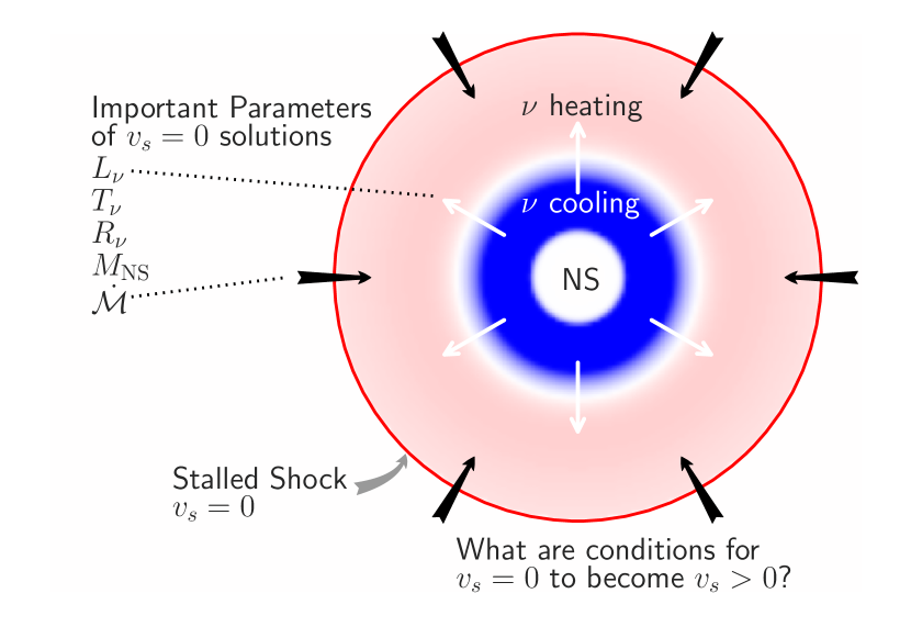
Figure 1: After the bounce shock stalls, the post-shock flow settles into a quasi-steady configuration. The solutions satisfy a boundary value problem between the neutron star “surface” and the stalled shock. The important parameters in determining the steady-state solutions are the neutrino luminosity being emitted from the core ($L_{\nu}$), the temperature of the neutrinos ($T_{\nu}$), the mass-accretion rate onto the shock and NS ($\dot{\mathcal{M}}$), the neutrino sphere or NS radius ($R_{\nu}$), and the NS mass ($M_{\rm NS}$). The fundamental challenge in core-collapse theory is to understand how $v_{s}=0$ transitions to $v_{s}>0$. In section 3, we derive such a condition.

3 Deriving an Integral Condition for $v_{s}>0$

We reduce the core-collapse problem to a set of integral conditions and show that this leads to a critical condition for explosions. Before we derive the integral conditions, let us describe what motivated us to consider the integral equations at all. The governing equations (eqs. 1-3) are commonly presented in differential form, but one could just as easily present them in integral form. The two forms represent exactly the same information. The choice is determined by the ease and method for finding solutions. For example, it is typically easier to work with the differential form when one needs to find numerical solutions, but if one seeks an analytic solution, the integral equations can be easier to use. For example, in finding the motion of a body in a potential field, one may solve the equations of motion, or one may use the integral condition, conservation of energy.

We argue that the integral equations provide an easier route to deriving a unified condition for explosions. Because the shock is a crucial component of the core-collapse problem, when we derive the explosion condition we embark on a route that is similar to deriving the Rankine-Hugoniot shock jump conditions. The route to deriving these jump conditions involves using the integral equations in the context of a moving boundary, the shock.

3.1 The generic integral condition

As in deriving the Rankine-Hugoniot conditions, we start with the conservation equations and the Reynolds transport theorem (or Leibniz-Reynolds transport theorem). Consider a generic conserved quantity, $q$, which could represent a mass density, momentum density, energy density, etc. Generically, one may define the total conserved quantity in region $D(t)$ as $\int_{D(t)}q\,dV$ and the time-rate-of-change of this conserved quantity is $\frac{d}{dt}\left(\int_{D(t)}q\,dV\right)$. The Reynolds transport theorem decomposes this time-rate-of-change into an Eulerian component and a component that accounts for the motion of the boundaries of region $D(t)$:

$$\frac{d}{dt}\left(\int_{D(t)}q\,dV\right)=\int_{D(t)}\frac{\partial q}{\partial t}\,dV+\oint_{\partial D(t)}q{\bf v}_{b}\cdot d{\bf S}\,,$$ (5)

with $\partial D(t)$ the surface of this domain, $d{\bf S}$ the surface element, and ${\bf v}_{b}$ the velocity of the surface. To make use of the Reynolds transport theorem, we need an expression for the Eulerian time derivative, $\partial q/\partial t$. The conservation equation provides such an expression. A general conservation equation has the following form:

$$\frac{\partial q}{\partial t}+\nabla\cdot{\bf f}=s\,,$$ (6)

where ${\bf f}$ is the flux of $q$, and $s$ is a source/sink of $q$. With these two equations (eqs. 5 & 6) we may now proceed to derive the integral conditions.

To construct the appropriate boundary value problem, we must choose the appropriate boundaries. We consider a boundary value problem where the lower boundary is at $r_{1}$ and the upper boundary is at $r_{2}$. The overall problem is divided into two domains, with a different solution in each domain. The pre-shock solution is in the domain $(r_{s}(t),r_{2}]$, the post-shock solution is in the domain $[r_{1},r_{s}(t))$, and the two solutions are joined by the Rankine Hugoniot jump conditions at $r_{s}(t)$. With the boundaries defined, we now define the integral equations.

First, we integrate eq. (6) from $r_{1}$ to $r_{2}$, and since the boundaries are constant in time, we have

$$\frac{d}{dt}\left(\int^{r_{2}}_{r_{1}}q\,dV\right)=\int^{r_{2}}_{r_{1}}\frac{\partial q}{\partial t}\,dV=\int^{r_{2}}_{r_{1}}\left(-\nabla\cdot{\bf f}+s\right)\,dV\,.$$ (7)

Next, we rewrite the left-hand side of eq. (7) to explicitly express the shock radius. In order to do this, we must divide the integral into two regions, above and below the shock, and we use the Reynolds transport equation (eq. 5). This gives

$$\frac{d}{dt}\left(\int^{r_{2}}_{r_{1}}q\,dV\right)=v_{s}4\pi r_{s}^{2}(q_{s-\epsilon}-q_{s+\epsilon})\\ +\int^{r_{s}(t)}_{r_{1}}\frac{\partial q}{\partial t}\,dV+\int^{r_{2}}_{r_{s}(t)}\frac{\partial q}{\partial t}\,dV\,,$$ (8)

where $s-\epsilon$ and $s+\epsilon$ represent values just below and above the shock. From here on, we introduce a more compact nomenclature for the values below and above the shock with $q_{-}$ and $q_{+}$.

In the core-collapse problem, the pre-shock solution is nearly in free-fall and can be solved analytically. Therefore, the problem reduces to finding the post-shock solution subject to the lower boundary, the surface of the NS, and the upper boundary, the shock. Now, we take the limit that $r_{2}$ approaches $r_{s}(t)$. In this limit, we have the following simplifications:

$$\lim_{r_{2}\to r_{s}(t)}q_{2}=q_{+}\;{\rm and}\;\lim_{r_{2}\to r_{s}(t)}\int^{r_{2}}_{r_{s}(t)}\frac{\partial q}{\partial t}\,dV=0\,,$$ (9)

which, when inserted into eq. (8), results in the simpler integral equation

$$\frac{d}{dt}\left(\int^{r_{2}}_{r_{1}}q\,dV\right)=v_{s}4\pi r_{s}^{2}(q_{-}-q_{+})+\int^{r_{s}(t)}_{r_{1}}\frac{\partial q}{\partial t}\,dV\,.$$ (10)

By plugging eq. (10) into eq. (7), we arrive at the general integral equation

$$v_{s}4\pi r_{s}^{2}(q_{-}-q_{+})+\int^{r_{s}(t)}_{r_{1}}\frac{\partial q}{\partial t}\,dV=4\pi(f_{1}r_{1}^{2}-f_{+}r_{s}^{2})+\int^{r_{s}}_{r_{1}}s\,dV\,.$$ (11)

Note that if we take the limit that $r_{1}$ approaches $r_{s}$ from below, this reduces to the shock jump conditions, but if we retain $r_{1}$ at the neutron star surface, we have the general integral equations describing the post-shock structure. If we assume a steady profile of $q(r)$ between the neutron star, $r_{1}$, and the shock, $r_{s}$, then this reduces to

$$v_{s}4\pi r_{s}^{2}(q_{-}-q_{+})=4\pi(f_{1}r_{1}^{2}-f_{+}r_{s}^{2})+\int^{r_{2}}_{r_{1}}s\,dV\,.$$ (12)

Eq. (12) represents the integral condition that relates the shock velocity to the steady-state integrals. For the core-collapse problem, there is not one constraint, but three that come from the three equations of hydrodynamics. In principal, this could be a messy algebraic problem to relate $v_{s}$ to the integral conditions. However, in the next section, we show that, in the context of the core-collapse problem, a simple relation emerges between the shock velocity and the integral conditions.

3.2 Deriving an expression for $v_{s}$ in terms of the integral conditions

Now, to derive the simple relation for the shock velocity in terms of the integral condition. We begin by summarizing the traditional way of deriving the shock velocity in terms of the density jump and pressure jump. Then, we use a similar technique, but instead of the pressure jump, we consider the full momentum integral. The Rankine-Hugoniot jump conditions in mass and momentum are

$$\rho_{-}u_{-}=\rho_{+}u_{+}$$ (13)

and

$$P_{-}+\rho_{-}u_{-}^{2}=P_{+}+\rho_{+}u_{+}^{2}\,,$$ (14)

where once again $\rho$ is the density and $P$ is the pressure. This time, however, $u=v-v_{s}$ represents the velocity in the shock frame, which, pragmatically, is just the difference in the lab frame velocity ($v$) and the shock velocity. As before, $+$ denotes the pre-shock state and $-$ denotes the post-shock state. Combining these two equations leads to the following expression for the shock velocity:

$${\rm v}_{s}=\frac{v_{s}}{{\rm v}_{+}}=-1+\sqrt{\frac{\beta(P_{-}-P_{+})}{(\beta-1)\rho_{+}v_{+}^{2}}}\,,$$ (15)

where ${\rm v}_{s}$ is the dimensionless shock velocity, scaled by the pre-shock speed, ${\rm v}_{+}=-v_{+}$, and $\beta=\rho_{-}/\rho_{+}$ is the shock compression ratio. In deriving eq. (15), there are formally two solutions, one with $+$ and one with $-$ in front of the radical sign. One of these solutions is real and the other is unphysical. The solution associated with $-$ corresponds to $P_{-}-P_{+}<0$ when $\rho_{-}-\rho_{+}>0$; this would result in a discontinuous rarefaction wave, which is unphysical. The other solution with $+$ in front of the radical sign corresponds to $P_{-}-P_{+}>0$ when $\rho_{-}-\rho_{+}>0$; this is a shock, the only physical solution.

So far, our derivation of eq. (15) is merely a summary and does not incorporate the integral conditions; now we use a similar procedure to derive an integral condition for the shock velocity. In deriving eq. (15), we began with the mass and momentum jump conditions across the shock; to derive the integral equivalent, we begin with the mass and momentum integral equations for the shock velocity. Using the generic integral equation, eq. (12), and the mass equation, eq. (1), the integral equation for mass that includes the shock is

$$v_{s}r_{s}^{2}(\rho_{-}-\rho_{+})=\rho_{1}v_{1}r_{1}^{2}-\rho_{+}v_{+}r_{s}^{2}\,$$ (16)

where the subscript $1$ denotes the state at the lower boundary, which in the core collapse case is the NS surface or neutrino sphere. The momentum equation, eq. (2), in combination with the generic integral equation, eq. (12), yields

$$v_{s}r_{s}^{2}(\rho_{-}v_{-}-\rho_{+}v_{+})=(P_{1}+\rho_{1}v_{1}^{2})r_{1}^{2}-(P_{+}+\rho_{+}v_{+}^{2})r_{s}^{2}\\ +\int^{r_{s}}_{r_{1}}2Pr\,dr-\int^{r_{s}}_{r_{1}}GM\rho\,dr\,.$$ (17)

In deriving these equations, we have made our first major assumption; the solutions between the neutron star and the shock are steady. This implies, for example, that $\rho_{1}v_{1}r_{1}^{2}=\rho_{-}v_{-}r_{s}^{2}$, but this does not necessarily imply that $\rho_{-}v_{-}=\rho_{+}v_{+}$. For the sake of brevity, we express the right-hand side of Eq. (17) as $\widetilde{\Psi}$.

$$\widetilde{\Psi}=(P_{1}+\rho_{1}v_{1}^{2})r_{1}^{2}-(P_{+}+\rho_{+}v_{+}^{2})r_{s}^{2}\\ +\int^{r_{s}}_{r_{1}}2Pr\,dr-\int^{r_{s}}_{r_{1}}GM\rho\,dr\,.$$ (18)

In the limit of low velocities behind the shock, $\widetilde{\Psi}$ is simply the overpressure behind the shock compared to hydrostatic equilibrium. The utility of using $\widetilde{\Psi}$ is that it incorporates the entire integral solution, including the boundary conditions.

The left-hand side of Eq. (17) must also satisfy the momentum jump condition, implying that

$$\widetilde{\Psi}=(P_{-}+\rho_{-}v_{-}^{2}-P_{+}-\rho_{+}v_{+}^{2})r_{s}^{2}\,.$$ (19)

Substitution of this equation into eq. (15) leads to the following dimensionless equation for the shock velocity

$${\rm v}_{s}=-1+\sqrt{\frac{\beta-\left(\frac{\rho_{-}v_{-}}{\rho_{+}v_{+}}\right)^{2}}{\beta-1}+\frac{\widetilde{\Psi}\beta}{(\beta-1)\rho_{+}v_{+}^{2}r_{s}^{2}}}\,,$$ (20)

where $\beta$ is the compression of density across the shock. While formally, this expression is correct within our given assumptions, its relative complexity hides its utility. With some simple assumptions, we produce a much simpler expression between ${\rm v}_{s}$ and $\widetilde{\Psi}$. First, note that in the strong shock limit, the ratio of densities, $\beta$, does not change as much as the jump in pressure, so that the variation of $\widetilde{\Psi}$ dominates the variation in ${\rm v}_{s}$. If the dynamics of the shock were merely dominated by a gamma-law EOS with $\gamma=4/3$, then the shock compression would be $\beta=7$. However, photodissociation of Fe and He nuclei at the shock alters the energetics as material passes through the shock. This loss of thermal energy causes a large shock compression. For more details on this, see Fernández & Thompson (2009), for example. As a result, the shock compression in most core-collapse situations is $\beta\sim 9$. With such a high shock compression, terms such as $\beta-1\sim\beta$, which further reduces the complexity in eq (20). Therefore, with fairly reasonable approximations, eq. (20) reduces to this more illuminating expression

$${\rm v}_{s}\approx-1+\sqrt{1+\Psi}\,,$$ (21)

where $\Psi=\widetilde{\Psi}/(\rho_{+}v_{+}^{2}r_{s}^{2})$ is the dimensionless overpressure normalized by the pre-shock ram pressure $\rho_{+}v_{+}^{2}r_{s}^{2}$. In this form, it is clear that when $\Psi>0$, the shock velocity is greater than zero, ${\rm v}_{s}>0$.

4 Validating the Steady-State Assumption and $\Psi\geq 0$ with one-dimensional parameterized simulations

Later, we use $\Psi$ to propose an explosion diagnostic for core-collapse simulations, but first we verify in this section that $\Psi=0$ during the stalled-shock phase and that $\Psi>0$ during explosion. To perform these validating tests, we calculate $\Psi$ in one-dimensional parameterized simulations.

The one-dimensional simulations are calculated using the new code Cufe, which will be described fully in J. W. Murphy & E. Bloor (in preparation). Cufe solves the equations of hydrodynamics eqs. (1-3) using higher-order Godunov techniques. The grid is logically Cartesian, but employs a generalized metric allowing for a variety of mesh geometries. For this study, we use spherical coordinates. The progenitor model is the 12 M_⊙ model of Woosley & Heger (2007), the EOS includes effects of dense nucleons around and above nuclear densities, nuclear statistical equilibrium, electrons, positrons, and photons (Hempel et al., 2012). For the neutrino heating, cooling, and electron capture we use the approximate local descriptions of Janka (2001) and Murphy et al. (2013).

We recall that there are five important parameters that describe the steady-state accretion solutions: $L_{\nu}$, $T_{\nu}$, $M_{\rm NS}$, $R_{\nu}$, and $\dot{\mathcal{M}}$. Two of these, $L_{\nu}$ and $T_{\nu}$, we set in the parameterized simulations; the rest we calculate self-consistently given the equations of hydrodynamics, the progenitor structure, and the EOS. The top panel of Figure 2 shows the time evolution of $M_{\rm NS}$, $R_{\nu}$, and $\dot{\mathcal{M}}$; we highlight the post-bounce phase of a model that does not explode. $\dot{\mathcal{M}}$ starts quite high, well above 1 M_⊙/s, but then drops down to $\sim$ 0.2 M_⊙/s near the end of the simulation. At around 500 ms after bounce, $\dot{\mathcal{M}}$ has a significant drop, which is a result of a density shelf advecting through the shock. Throughout this paper, you will notice that this significant drop in $\dot{\mathcal{M}}$ becomes imprinted on many of the explosion diagnostics, including the shock radius vs. time in the bottom panel of Figure 2.

When compared to more realistic simulations (Melson et al., 2015, see Figure 4), $R_{\nu}$ evolves very little during the time shown in Figure 2. This is a known drawback of the standard light-bulb prescription, but it does not impact the qualitative conclusions that we present later. In more realistic calculations such as Melson et al. (2015), the proto-neutron star contracts for two reasons. For one, as matter piles onto the PNS, the neutron star compresses a little. The primary reason that the proto-neutron star contracts, however, is that the core neutrino luminosity cools the neutron star. In our neutrino model, we omit the diffusive cooling of neutron star. Hence, our core only contracts as a result of the added weight of matter.

However, because each moment may be modeled as a successive set of steady-state solutions, this lack of contraction does not affect our general conclusion that we may calculate an explodability parameter. Later, we will calculate an explodability parameter that depends upon the five parameters, $R_{\nu}$ being one of them. Because the solutions are time independent, the explodability parameter calculation is also time independent. Each moment in time has its own explodability value that is independent of any other moment. Therefore, it does not matter what the evolutionary history of $R_{\nu}$ is; we are able to calculate the explodability parameter for any neutrino-sphere radius history.

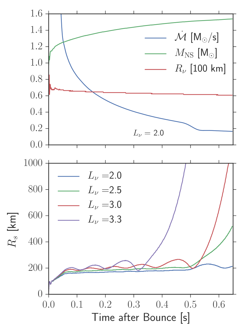
Figure 2: Characteristics of one-dimensional parameterized simulations. Top panel: mass-accretion rate ($\dot{\mathcal{M}}$), mass of neutron star ($M_{\rm NS}$), and neutrino sphere or radius of neutron star ($R_{\nu}$) vs. time for the lowest luminosity simulation. Later we compare the integral condition for explosion with parameterized simulations. Here, we show the three important parameters of the steady-state problem highlighted in Figure 1, which are calculated self-consistently in the simulations. The evolution of these parameters with time is similar for all simulations, therefore we only show the lowest luminosity simulation here. Bottom panel: shock radius ($R_{s}$) vs. time for four one-dimensional parameterized simulations. To facilitate comparison with the integral condition, we parameterize the neutrino heating and cooling. The neutrino luminosities are in units of $10^{52}$ erg s^-1.

To sample a range of explosion timescales, we vary the light-bulb neutrino luminosity, $L_{\nu}$. The bottom panel of Figure 2 shows the resulting shock radii vs. time labeled by $L_{\nu}$ in units of $10^{52}$ erg s^-1. In all models, the shock forms at 153 ms after the start of the simulations and quickly stalls between $\sim$150 to $\sim$200 km. The general trend is that the higher luminosity models explode earlier than lower luminosity models. The lowest luminosity model does not explode at all. However, it does experience a significant outward adjustment and oscillation of the shock as $\dot{\mathcal{M}}$ drops significantly around 500 ms after bounce. The $L_{\nu}=2.5$ & 3.0 models explode during the advection of the density shelf. An obvious feature present in the shock radius evolution plot are the shock radius oscillations. They are often present in one-dimensional simulations near explosion (Ohnishi et al., 2006; Buras et al., 2006b; Murphy & Burrows, 2008), and Fernández (2012) suggests that they might be related to the advective-acoustic feedback loop that is responsible for the standing accretion shock instability (SASI) in multi-dimensional simulations.

Our first task is to verify one of the primary results of this manuscript, the relationship between ${\rm v}_{s}$ and the integral quantity $\Psi$, eq. (21). Figure 3 plots the shock velocity normalized by the pre-shock in-fall speed, ${\rm v}_{s}=v_{s}/{\rm v}_{+}$, for the $L_{\nu}=3.0$ model. For comparison, we plot the right-hand side of eq. (21), $-1+\sqrt{1+\Psi}$, where $\Psi$ is calculated directly from the simulation. For the most part, the curves agree, validating our derivation and assumptions.

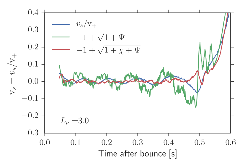
Figure 3: Normalized shock velocity vs. time after bounce. This plot validates the assumptions and derivation of eq. (21), which relates the shock velocity ${\rm v}_{s}$ to pressure integral condition $\Psi$. ${\rm v}_{s}$ is the shock velocity normalized by the the pre-shock in-fall speed, ${\rm v}_{+}$, and $\Psi$ is overpressure behind the shock in integral form. When $\Psi\approx 0$, ${\rm v}_{s}\approx 0$, and when $\Psi>0$, ${\rm v}_{s}>0$. This validation sets the stage for the explodability condition in Figure 8.

Next, we validate the steady-state assumption. Before we do so, we need to consider how time dependence might affect eq. (21). In steady-state, the momentum integral equation is $v_{s}r_{s}^{2}(\rho_{-}v_{-}-\rho_{+}v_{+})=\widetilde{\Psi}$, but if we include the time-dependent term, then the momentum integral equation is

$$v_{s}r_{s}^{2}(\rho_{-}v_{-}-\rho_{+}v_{+})=\widetilde{\chi}+\widetilde{\Psi}\,,$$ (22)

where

$$\widetilde{\chi}=\int_{r_{1}}^{r_{s}-\epsilon}\frac{\partial(\rho v)}{\partial t}\,dV\,,$$ (23)

and $r_{1}$ is the size of the proto-neutron star, or neutrino-sphere radius. Our goal is to see how this time-derivative term affects our expression for the shock velocity, therefore we use eq. (22) in our derivation for the shock velocity in section 3.2. The equivalent of the final result, eq. (21), is

$${\rm v}_{s}\approx-1+\sqrt{1+\Psi+\chi}\,,$$ (24)

where $\chi$ is just $\widetilde{\chi}$ normalized by $\rho_{+}v_{+}^{2}r_{s}^{2}$.

In some sense, Figure (4) has validated Equation (21) in which we ignored the time-derivative term, so that it already hinted that $\chi$ would be small. To be certain that $\chi\approx 0$, we compare $\Psi$ and $\chi$ in Figure (4). In general, $(1+{\rm v}_{s})^{2}-1=\Psi+\chi$, but if $\chi\approx 0$, then we expect $(1+{\rm v}_{s})^{2}-1\approx\Psi$. During the steady-state phase, when the average shock velocity is zero, we find that both $\Psi$ and $\chi$ are small and approximately zero. In fact, their small amplitudes nearly cancel. During the initiation of the explosion, $\Psi$ grows substantially, but $\chi\approx 0$. Later, when the explosion really takes off, both $\chi$ and $\Psi$ are important. Interestingly, we find that assuming steady-state is a valid approximation during the steady-state phase and the initiation of the explosion, but once explosion commences in earnest, one must clearly consider a time-dependent evolution. The focus of this manuscript is in deriving a condition for the initiation of explosion, however, in which case Figure 3 suggests that eq. (21) is a fine place to start.

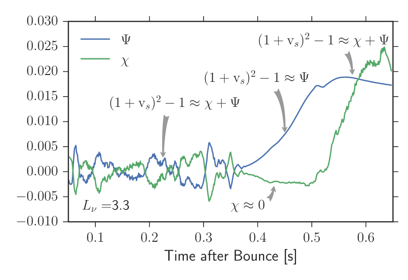
Figure 4: Checking that steady-state is a reasonable assumption in the integral condition. Here we show the overpressure, $\Psi$ and time-derivative of momentum, $\chi$, as a function of time after bounce. During the stalled-shock phase, the average shock velocity is very nearly zero, and $\Psi$ and $\chi$ oscillate about zero as the shock oscillates. Even with these oscillations, both $\Psi$ and $\chi$ are quite small. During the initial stages of explosion, $\chi\approx 0$, and the amplitude of the shock velocity is best represented by $\Psi$ alone. Later, as the explosion proceeds vigorously, both $\Psi$ and $\chi$ contribute to the velocity. Since we are concerned with the revival phase of the shock, we find that steady-state is a reasonable approximation during initiation of the explosion.

In Figure 5, we show $\Psi$ for all of the models that we considered. $\Psi$ is indeed zero during the steady-state phase and $\Psi>0$ during explosion. The fact that simulations roughly validate $\Psi\geq 0$ implies that $\Psi$ is a good dimensionless explosion diagnostic.

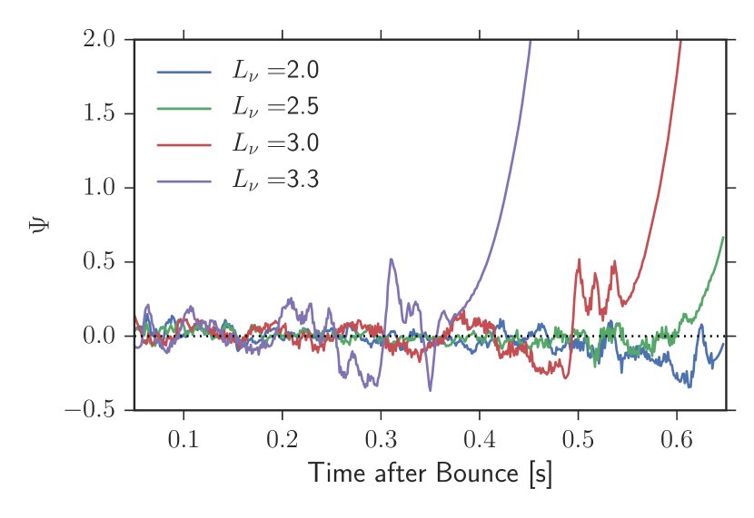
Figure 5: $\Psi$, the integral explosion condition, evaluated from the one-dimensional simulations as a function of time. In section 3, we derive an integral condition for explosion based upon the momentum equation; we derive that $v_{s}\geq 0$ corresponds to $\Psi\geq 0$. To test whether this condition corresponds to explosion, we evaluate $\Psi$ for the one-dimensional parameterized simulations described in section 4; we find that $\Psi=0$ during the stalled-shock phase, and $\Psi>0$ during explosion. These results strongly suggest that $\Psi\geq 0$ is a useful condition for explosion. However, this condition does not by itself predict explosion. It only indicates that explosion has occurred. In section 5, we propose a method to turn $\Psi\geq 0$ into a useful explosion diagnostic.

5 $\Psi_{\rm min}$: A nearness-to-explosion condition

The fact that $\Psi>0$ during explosion (Figure 5) suggests that $\Psi$ has the potential to be a good explosion diagnostic. However, just calculating $\Psi$ from the simulations is not the most useful condition; $\Psi$ remains near zero during the non-exploding phase, and it only deviates from zero while the simulation is exploding. This behavior is not a very useful explosion diagnostic, and one might as well only use the shock radius. In fact, most explosion “conditions” or “diagnostics” to date have this problem. They do not provide a nearness-to-explosion condition. What we need is a way to translate the $\Psi\geq 0$ condition into a useful nearness-to-explosion condition. Fortunately, $\Psi$ lends itself to such an explosion diagnostic.

Our strategy for developing a nearness-to-explosion condition is to extract $L_{\nu}$, $T_{\nu}$, $R_{\nu}$, $M_{\rm NS}$, and $\dot{\mathcal{M}}$ from the simulations and calculate the quasi-steady-state solutions for this set of parameters. For a given set of parameters, there is a family of solutions to the quasi-steady-state equations, each with a different shock radius. Each solution has a value for $\Psi$ which may be $<0$, $=0$, or $>0$, which corresponds to solutions with $v_{s}<0$, $v_{s}=0$, or $v_{s}>0$, respectively. The $v_{s}=0$ ($\Psi=0$) solution is a quasi-equilibrium solution. We will show that for each family of solutions, there is always a minimum $\Psi$, which we denote $\Psi_{\rm min}$. When $\Psi_{\rm min}<0$, then $v_{s}=0$ solutions exist. However, when $\Psi_{\rm min}>0$, the only solutions that exist have $v_{s}>0$. Therefore, we propose that $\Psi_{\rm min}$ is an excellent explosion diagnostic providing a nearness-to-explosion condition. Figures 6 & 7 illustrate these points.

Having outlined the strategy, we now provide the specifics in calculating $\Psi_{\rm min}$. We begin with the steady-state equations

$$\dot{M}=4\pi r^{2}\rho v\,,$$ (25)

$$\rho\frac{dv}{dr}+\frac{dP}{dr}=-\rho\frac{\phi}{r}\,$$ (26)

and

$$\frac{\dot{M}}{4\pi r^{2}}\frac{d\varepsilon}{dr}+P\frac{d(r^{2}v)}{r^{2}dr}=\rho q\,.$$ (27)

To solve these equations, we need an EOS to relate P in terms of $\varepsilon$ and $\rho$, and we need boundary conditions. For the region that we consider, above the neutrino sphere and below the shock, the dominant contributors to the EOS are neutrons, protons, helium nuclei ($\alpha$), positrons, electrons, and photons. Because this region is not dominated by dense nuclear physics, the EOS is more straightforward and for the most part analytic. Eventually, we hope to translate the results of this manuscript into an analytic solution for the conditions for explosion. To facilitate that later goal, we use the analytic EOS now. We treat the neutrons, protons, and $\alpha$s as an ideal nonrelativistic gas; the positrons, electrons, and photons constitute the relativistic part of the plasma, and we consider the positrons and electrons in an arbitrary degeneracy. To calculate the relative abundances of neutrons, protons, and $\alpha$s, we assume nuclear statistical equilibrium for these three components and use the Saha equation to calculate their abundances. See appendix B for the details in calculating the EOS and the abundances.

In the spirit of Burrows & Goshy (1993) and others (Yamasaki & Yamada, 2005, 2006; Yamasaki & Foglizzo, 2008), we solve the steady-state equations, Eqs. (25-27), using the Rankine-Hugoniot jump conditions for a stalled shock. The jump conditions give the post-shock state (subscript $-$) in terms of the pre-shock state (subscript $+$):

$$\rho_{-}v_{-}=\rho_{+}v_{+}\,,$$ (28)

$$\rho_{-}v_{-}^{2}+P_{-}=\rho_{+}v_{+}^{2}+P_{+}\,,$$ (29)

and

$$h_{-}+\frac{v_{-}^{2}}{2}=h_{+}+\frac{v_{+}^{2}}{2}\,.$$ (30)

For the pre-shock state, we make the following assumptions that enable analytic solutions of the conditions. First, we assume that $\dot{\mathcal{M}}=4\pi r_{s}^{2}\rho_{+}v_{+}$ is a constant. Second, we assume that the star is accreting onto the shock at a large fraction of free fall, so the pre-shock speed is given by $v_{+}^{2}=2\alpha_{v}\phi(R_{s})$, where $\phi(R_{s})$ is the potential at the shock radius, and $\alpha_{v}$ is the fraction of free-fall. Third, we assume that the pre-shock Bernoulli constant is roughly zero, $h_{+}+v_{+}^{2}-\phi(R_{s})\approx 0$. Finally, we assume a gamma-law relationship for the pre-shock pressure, internal energy, and density: $\gamma_{4}\equiv P/(\rho\varepsilon)+1$. Under these assumptions, the pre-shock pressure is

$$P_{+}=\frac{\gamma_{4}\rho_{2}(1-\alpha_{v})}{\gamma_{4}-1}\phi(R_{s})\,.$$ (31)

Specifying $\dot{\mathcal{M}}$, $\alpha_{v}$, $\gamma_{4}$, and $R_{s}$ then sets the boundary conditions at the shock. When Burrows & Goshy (1993) first introduced the critical luminosity, they specified one more boundary condition at the base: $\tau=\int\kappa\rho dr=2/3$. This extra condition enables one to self-consistently solve for the shock radius that permits a steady-state-stalled-shock solution. Yamasaki & Yamada (2005) noted that the density at the radius where $\tau=2/3$ is almost always the same, so that one can easily replace the $\tau$ condition by specifying a specific density, $\rho_{2/3}$, at the neutrino sphere, or neutron star surface. The traditional way to find the critical curve is to look for solutions that satisfy $\rho_{1}=\rho_{2/3}$; above a curve in luminosity and accretion-rate space there are no solutions that satisfy this condition. Burrows & Goshy (1993) interpreted this as a critical condition for explosion. However, it has never been clear why this condition on the inner density should naturally lead to a critical condition for explosion. Now, we show that the solutions above the curve indeed only have solutions that correspond to ${\rm v}_{s}>0$.

To do this, we show that a condition on the inner boundary, $\rho_{2/3}/\rho_{1}>1$, is equivalent to $\Psi>0$ and ${\rm v}_{s}>0$. Historically, the method for finding the critical curve is as follows. First, for a given $R_{s}$, one finds “solutions” to the steady-state equations by starting with the $v_{s}=0$ jump conditions at the shock and integrating steady-state equations inward to the inner boundary. The resultant partial solution satisfies the governing equations except that they do not necessarily satisfy the inner boundary condition, which means that they are not a true solution. One then finds the true solution by modifying the shock radius until the partial solution also gives the correct inner boundary condition. One may use these partial solutions at any shock radius to infer what $v_{s}$ would be as a function of $R_{s}$.

Understanding the density profile and pressure profiles of these partial solutions is the key to connecting the old condition on the inner density with a condition on $v_{s}$. Note that $\Psi$ in eq. 21 depends upon $P_{1}$, $\rho$, and $\rho_{1}$. If one could specify analytic solutions for the pressure and density profile, then the condition would be analytic. In a future paper (J. W. Murphy & J. C. Dolence, in preparation), we will do just that. For now, we use the numerical solutions to the steady-state equations to propose a semi-analytic solution for the explosion condition. It is our experience that the density profile of the partial solution is similar for a given set of parameters and $R_{s}$. In other words, the density profile may be written as $\rho(r)=\rho_{1}z(r)$. Furthermore, a natural dimensionless expression relating the density and pressure is $y=P/(\rho\phi)$, and we find that the shape and scale of $y$ mostly depends on the five parameters and $R_{s}$. Therefore, we find that $P$ is also proportional to $\rho_{1}$ via $P=\rho_{1}y(r)z(r)\phi(r)$. Substituting these expressions for $\rho$ and $P$ into the expression for $\widetilde{\Psi}$ (Equation 18), one finds that

$$\widetilde{\Psi}=\rho_{1}f-P_{+}r_{s}^{2}-\rho_{+}v_{+}^{2}r_{s}^{2}\,,$$ (32)

where $f$ incorporates $y(r)$, $z(r)$, and $\phi(r)$ in the first, third, and fourth terms of eq. (18). When one integrates the steady-state equations, one naturally finds that $\widetilde{\Psi}=0$ but the inner density $\rho_{1}$ is not necessarily equal to the desired inner boundary, $\rho_{2/3}$. Because $\rho=\rho_{1}z(r)$, then we may easily substitute $\rho_{2/3}$ to see how $\widetilde{\Psi}$ changes when we demand that $\rho_{1}=\rho_{2/3}$. In terms of $\rho_{1}$, the inner density of the partial solution, and $\rho_{2/3}$, the desired inner boundary, the dimensionless overpressure becomes

$$\frac{\widetilde{\Psi}}{(P_{+}+\rho_{+}v_{+}^{2})r_{s}^{2}}=\frac{\rho_{2/3}}{\rho_{1}}-1\approx\Psi\,,$$ (33)

where the final approximation comes about because the pre-shock pressure is typically much lower than the ram pressure, $P_{+}\ll\rho_{+}v_{+}^{2}$. By eq. (21), this approximate expression for $\Psi$ gives the following expression for the shock velocity in terms of the inner densities:

$${\rm v}_{s}\approx-1+\sqrt{\frac{\rho_{2/3}}{\rho_{1}}}\,.$$ (34)

This presents our final derivation to show that the solutions above the critical luminosity-accretion-rate curve have positive shock velocity. Before this derivation, Burrows & Goshy (1993) and many others suggested that the inability to find solutions that have $\rho_{1}=\rho_{2/3}$ implies explosion. In fact, our derivation implies the following explosion condition:

$$\frac{\rho_{2/3}}{\rho_{1}}>1\rightarrow\Psi>0\rightarrow{\rm v}_{s}>0\,.$$ (35)

To find $\Psi$ as a function of $R_{s}$, we use the one-dimensional simulations to inform the values for $\dot{\mathcal{M}}$, $M_{\rm NS}$, $R_{\nu}$, $\alpha_{v}$, and $\gamma_{4}$, and of course, we set $L_{\nu}$ and $T_{\nu}$ to the values used for the one-dimensional parameterized simulations. Then we find solutions to the steady-state equations for a wide range of shock radii. These solutions represent a family of solutions at different $R_{s}$ but all with the same parameters. For each solution and associated $R_{s}$, we evaluate $\Psi$ using eq. (33), where we follow Yamasaki & Yamada (2005) and set $\rho_{2/3}=7\times 10^{10}$ g cc^-1. Since ${\rm v}_{s}\approx-1+\sqrt{1+\Psi}$, $\Psi$ naturally shows which solutions have $v_{s}<0$, $v_{s}=0$, or $v_{s}>0$. The $v_{s}=0$ solution corresponds to the steady-state-stalled-shock solution.

Figure 6 shows the outcome of this process. Each line corresponds to a specific set of parameters and one family of solutions. For clarity, we only vary $L_{\nu}$ between different families of solutions. For low values of $L_{\nu}$, all three solutions ($v_{s}>0$, $v_{s}=0$, and $v_{s}<0$) are possible. For low $R_{s}$, $\Psi>0$, implying that $v_{s}>0$ and the shock would move outward. For larger $R_{s}$, $\Psi<0$ so that $v_{s}<0$ and the shock would tend to move inward. In between, at a very specific shock radius, there is a solution that has $\Psi=0$ and $v_{s}=0$. This solution represents an equilibrium solution. While solutions far from equilibrium are not steady and therefore are poorly represented by the steady-state equations, our approach does not rely on the quantitative accuracy of this representation. For a visual aide to these concepts, see Figure 7.

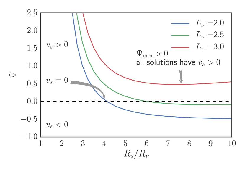
Figure 6: The family of steady-state solutions represented by their values of $\Psi(R_{s}/R_{\nu})$ for three different neutrino luminosities but all else being equal. For some parameters, $\Psi$ may be negative, zero, or positive. The solution with $\Psi=0$ ($v_{s}=0$) corresponds to the equilibrium solution. For each family, there is a solution with a minimum $\Psi$, which we denote $\Psi_{\rm min}$. When $\Psi_{\rm min}<0$, a stalled-shock ($v_{s}=0$) solution exists, but when $\Psi_{\rm min}>0$, only solutions with $v_{s}>0$ exist. We propose that $\Psi_{\rm min}>0$ is an excellent explosion diagnostic (see Figure 8).

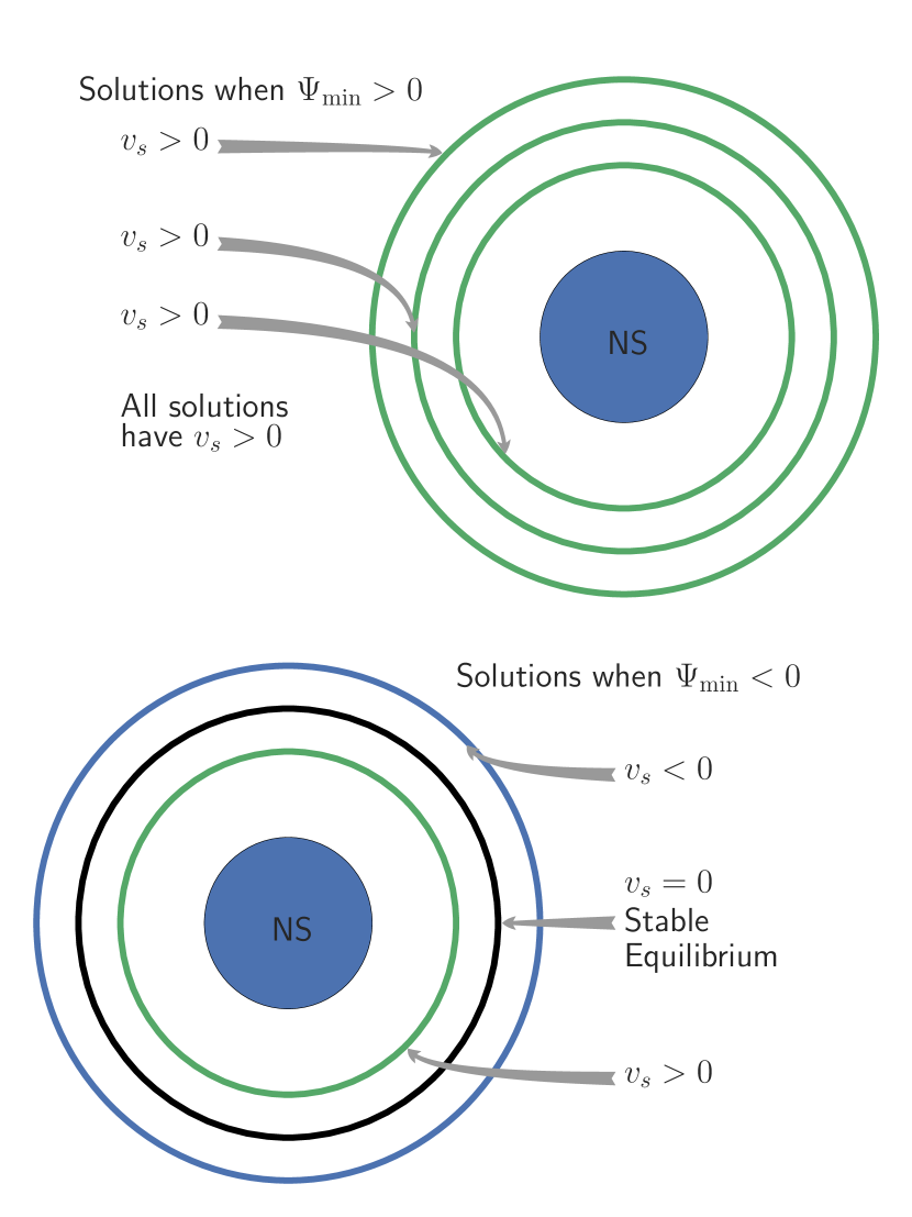
Figure 7: This is an illustration to demonstrate the two regimes seen in Figure 6. If $\Psi_{\rm min}<0$, then there are solutions with $v_{s}<0$, $v_{s}=0$, and $v_{s}>0$. In general, the solution with $v_{s}=0$ is an equilibrium solution, and as long as it exists, simulations (and presumably Nature) settle on this steady-state stalled-shock solution. When $\Psi_{\rm min}>0$, the only solutions are those in which $v_{s}>0$. Therefore, $\Psi_{\rm min}$ seems to be a natural condition for explosion.

Note that for high values of $L_{\nu}$ there are no solutions for which $\Psi_{\rm min}<0$. In these cases, all solutions correspond to $v_{s}>0$. There is a very specific set of parameters for which $\Psi_{\rm min}=0$. The locus of such parameters defines a critical hypersurface that generalizes but encompasses the critical neutrino luminosity condition of Burrows & Goshy (1993) (see Section 6 for more on this).

To validate that $\Psi_{\rm min}$ satisfies the desired qualities of an explosion diagnostic, we plot $\Psi_{\rm min}$ in Figure 8 for the one-dimensional parameterized simulations. The parameters that we set by hand in each simulation are $L_{\nu}$ and $T_{\nu}$; we keep $T_{\nu}$ set at 4 MeV, and vary $L_{\nu}$. At each time, we extract the other important parameters $M_{\rm NS}$, $R_{\nu}$, and $\dot{\mathcal{M}}$, which are calculated self-consistently in the simulation. We then calculate the family of steady-state solutions for that set of parameters and find the value of $\Psi_{\rm min}$. Figure 8 shows that $\Psi_{\rm min}$ has the desired qualities of an explosion condition. Before explosion, $\Psi_{\rm min}<0$ and during explosion, $\Psi_{\rm min}>0$. Moreover, we suggest that the value of $\Psi_{\rm min}$ before explosion provides a useful metric for how far away the simulation is from explosion.

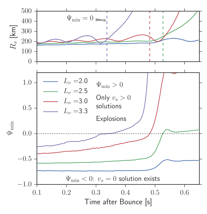
Figure 8: Nearness-to-explosion condition for one-dimensional hydrodynamic simulations: $\Psi_{\rm min}$ vs. time. For each time, we extract the important parameters of the problem ($L_{\nu}$, $T_{\nu}$, $R_{\nu}$, $M_{\rm NS}$, and $\dot{\mathcal{M}}$) from the one-dimensional hydrodynamic simulations and calculate the family of steady-state solutions. $\Psi_{\rm min}$ represents the minimum possible value of $\Psi$ over that family (see Figure 6). While $\Psi_{\rm min}<0$, there exists a stalled accretion shock solution ($\Psi=0$ and $v_{s}=0$). When $\Psi_{\rm min}>0$, all possible solutions have $v_{s}>0$, which we associate with explosion. Empirically, we find that before explosion $\Psi_{\rm min}<0$ and during explosion $\Psi_{\rm min}>0$. Most importantly, the value of $\Psi_{\rm min}$ offers an excellent indication of nearness-to-explosion.

6 Comparison with Other Explosion Conditions

In this section, we briefly compare the integral explosion diagnostic, $\Psi_{\rm min}$ with three other conditions: the critical neutrino luminosity condition (Burrows & Goshy, 1993), a timescale ratio condition (Janka & Keil, 1998; Thompson, 2000; Thompson et al., 2005; Buras et al., 2006a; Murphy & Burrows, 2008), and the antesonic condition (Pejcha & Thompson, 2012). In this manuscript, we mostly compare the effectiveness of these conditions with the integral condition; in a forthcoming paper (J. W. Murphy & J. C. Dolence, in preparation), we show that one can actually derive all three conditions from the integral condition by making various further approximations. For now, we simply compare the conditions.

Of these three, the most closely related condition is the critical luminosity condition of Burrows & Goshy (1993). In fact, a primary motivation in deriving the integral condition is to derive a condition that shows that the solutions above the critical neutrino luminosity curve correspond to $v_{s}>0$. In section 3, we derived the integral condition for $v_{s}>0$, and now, in the bottom left panel of Figure 9, we show that this same integral condition reproduces the critical neutrino luminosity curve of Burrows & Goshy (1993).

To reproduce the critical neutrino luminosity curve in the lower left panel of Figure 9, we first fix three of the five important parameters of the problem, $R_{\nu}$, $M_{\rm NS}$, and $T_{\nu}$. In other words, we restrict the dimensionality of the integral condition to the $L_{\nu}$-$\dot{\mathcal{M}}$ plane. Then we find the solutions to the steady-sate equations (eqs. 25-27) and select the solutions in the $L_{\nu}$-$\dot{\mathcal{M}}$ plane that have $\Psi_{\rm min}=0$. The locus of these specific solutions forms the solid curve that we show in Figure 9. Above this curve, $\Psi_{\rm min}>0$ and therefore all solutions have $v_{s}>0$. Below this curve, $\Psi_{\rm min}<0$, and therefore a steady-state stalled-shock solution exists. This curve is exactly the same critical neutrino luminosity curve that Burrows & Goshy (1993) and others have derived. The difference is in the way that it is derived. Burrows & Goshy (1993) solved the steady-state equations looking for solutions for which the shock and $\tau=2/3$ conditions are satisfied. There is no statement about the behavior of $v_{s}$ above the curve. Rather than highlighting $\tau$, we instead use the $\Psi_{\rm min}=0$ condition, that one readily sees that $v_{s}>0$ above the curve.

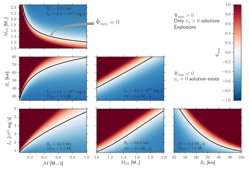
Figure 9: “Critical curves” defined by the $\Psi_{\rm min}=0$ condition. These plots show that the $\Psi_{\rm min}=0$ is another way to define the critical curve, the solutions above the critical curve have positive shock velocity, and the $L_{\nu}$-$\dot{\mathcal{M}}$ curve is merely a slice of a critical hypersurface. Each panel represents a two-dimensional slice through the five-dimensional parameter space. In all panels, $T_{\nu}$ is fixed to 4 MeV. The two other fixed parameters are labeled in each panel. The color map shows the value of $\Psi_{\rm min}$ as a function of the two remaining parameters, and the solid black line shows where $\Psi_{\rm min}=0$. In the lower left panel, we show that the $\Psi_{\rm min}=0$ condition produces the critical $L_{\nu}-\dot{\mathcal{M}}$ curve of Burrows & Goshy (1993). Note that above this curve $\Psi_{\rm min}>0$, which implies that solutions above the curve have $v_{s}>0$. In the context of our assumptions, this suggests that the solutions above the critical curve are explosive, as Burrows & Goshy (1993) initially suggested. Finally, with these panels, we show that the critical neutrino luminosity curve is a slice of a more general critical hypersurface. Most importantly, this critical hypersurface is represented by one dimensionless condition, $\Psi_{\rm min}=0$.

In addition to showing that $v_{s}>0$ above the critical neutrino luminosity curve, we also show that $\Psi_{\rm min}>0$ is a more general explosion condition than the critical $L_{\nu}$-$\dot{\mathcal{M}}$ curve. In fact, in the important parameters, $\Psi_{\rm min}=0$ represents a critical hypersurface, and the critical $L_{\nu}$-$\dot{\mathcal{M}}$ curve is just one slice of this more general critical condition. To help illustrate this, we use in Figure 9 the $\Psi_{\rm min}=0$ to derive other critical curves, where each is just a different slice of the critical hypersurface. Each critical curve is constructed in the same way as the $L_{\nu}$-$\dot{\mathcal{M}}$ critical curve, except that a different set of three parameters is fixed. In all panels, $T_{\nu}$ is fixed to 4 MeV; each panel shows the values for the other two parameters. In the past, the literature has focused on the $L_{\nu}$-$\dot{\mathcal{M}}$ critical curve, mostly because that is how this useful critical curve was discovered and presented (Burrows & Goshy, 1993). However, Figure 9 clearly shows that there are many other critical curves, one for each pair of the five parameters.

By focusing on one critical curve, one runs the danger of overemphasizing two of the parameters and underemphasizing the other three parameters. For example, the $L_{\nu}$-–$\dot{\mathcal{M}}$ critical curve suggests that one should pay attention to the evolution of $L_{\nu}$ and $\dot{\mathcal{M}}$. When it comes to the equations, however, there is nothing special about $L_{\nu}$ or $\dot{\mathcal{M}}$; all parameters are potentially important. Depending upon the evolution of the parameters, it might therefore be more instructive to consider the evolution of, for example, $R_{\nu}$ and $\dot{\mathcal{M}}$.

The $\Psi_{\rm min}=0$ critical condition suggests another way to view the nearness-to-explosion that does not overemphasize any one parameter. The five parameters define a five-dimensional hyperspace, and the $\Psi_{\rm min}=0$ condition defines a hypersurface within the five-dimensional space. Below the $\Psi_{\rm min}=0$ hypersurface, steady-state solutions exist, and above this hypersurface we show that the solutions are likely explosive. As a simulation evolves, it will trace out a path in this 5-dimensional hyperspace, and in general, it will move toward or away from the $\Psi_{\rm min}=0$ hypersurface. Therefore, a generalized distance to this surface would be an excellent measure of nearness-to-explosion. In a future paper, we will present discussions of this generalized distance. For now, we merely introduce this new concept, and propose that since the value of $\Psi_{\rm min}$ defines the hypersurface, it is a good proxy for the generalized distance to the bounding hypersurface. This definition is useful for two reasons. One, since the hypersurface is defined by $\Psi_{\rm min}=0$, we are able to define the critical condition by one dimensionless parameter and not five. Two, this dimensionless parameter is intimately related to a fundamental question of CCSN theory. $\Psi$ is proportional to $v_{s}$, and a fundamental question of CCSN theory is “what are the conditions for $v_{s}>0$?” Hence a single dimensionless parameter, $\Psi_{\rm min}$, that defines the condition for explosion is also intimately related to an important question in CCSN theory.

To help illustrate the critical hypersurface, Figure 10 shows two slices of this hypersurface. Since it is difficult to visualize a five-dimensional hypersurface, we instead show two slices of the hypersurface. In the top panel of Figure 10, we fix $T_{\nu}$ to 4 MeV and $R_{\nu}=63$ km. The resulting surface is a two-dimensional surface defined by three dimensions. In each of the axis planes, we also show critical curves, with each curve corresponding to a specific value of the third axis. The bottom panel shows an equivalent slice, but this time the slices are at $T_{\nu}=4$ MeV and $L_{\nu}=3\times 10^{52}$ erg/s. While it is impossible to show the full hypersurface, we hope to illustrate with these two-dimensional slices that the critical condition is not only a critical curve, but a critical hypersurface defined by $\Psi_{\rm min}=0$. Below the hypersurface, $\Psi_{\rm min}<0$, and steady-state solutions exist; above the hypersurface, $\Psi_{\rm min}>0$ and all solutions likely have $v_{s}>0$.

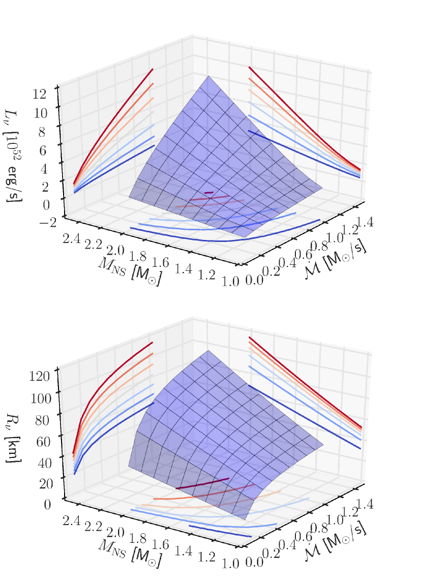
Figure 10: Critical hypersurface for explosion. The $\Psi_{\rm min}=0$ condition defines a hypersurface in the five-dimensional parameter space. Below the hypersurface, $\Psi_{\rm min}<0$, and steady-state solutions exist; above the hypersurface, $\Psi_{\rm min}>0$. Therefore, only solutions with $v_{s}>0$ exist. It is difficult to visualize the full hypersurface; therefore we present two slices that are themselves two-dimensional surfaces. In both plots, we fixed $T_{\nu}$ to 4 MeV. In the top plot, we also fixed $R_{\nu}$ to 63 km, and in the bottom plot we fixed $L_{\nu}$ to $3\times 10^{52}$ erg s^-1. We also show “critical curves,” for which we specify the value for the third dimension.

Another common class of explosion metrics are the timescale ratios in which one compares an advection timescale ($\tau_{\rm adv}$) to a heating timescale ($\tau_{\rm heat}$). Roughly, neutrino heating might be expected to significantly modify the internal energy of the accreting material only when $\tau_{\rm heat}\lesssim\tau_{\rm adv}$. Based on this, many have used the ratio $\tau_{\rm adv}/\tau_{\rm heat}$ as a diagnostic to indicate how close a model is to explosion for a given snapshot (Janka & Keil, 1998; Thompson, 2000; Thompson et al., 2005; Buras et al., 2006a; Murphy & Burrows, 2008). While this may seem sensible at face value, the timescale ratio arguments all neglect important aspects of the CCSN problem — cooling that occurs below the gain region, for example. Meanwhile, Murphy & Burrows (2008) and others more recently (Dolence et al., 2013; Takiwaki et al., 2014; Hanke et al., 2012) have shown that the turbulent dynamics of multidimensional lead to longer advection times on average, speculating that this may be an important effect vis-à-vis 1D vs. multi-D.

There are many approximate definitions of $\tau_{\rm adv}$ and $\tau_{\rm heat}$ (Janka & Keil, 1998; Murphy & Burrows, 2008; Fernández, 2012) . Early definitions of the advection time include $\tau_{\rm adv}=\int_{r_{\rm gain}}^{r_{\rm shock}}dr/v_{r}$, but the most recent definitions use the mass in the gain region and the mass-accretion rate

$$\tau_{\rm adv}=\frac{M_{\rm gain}}{\dot{\mathcal{M}}}\,.$$ (36)

For the rest of this paper, we adopt this most recent definition. For the heating timescale, the generic approach is to compare a total energy with an integrated heating rate $\tau_{\rm heat}=E/Q$. Generically, many define the heating rate as $Q=\int_{\rm gain}(H-C)\rho\,dV$. The total energy has several definitions, and since none are derived from a firm explosion condition, all are arbitrary. We highlight and use one condition; we consider the total internal energy in the gain region $E=\int_{\rm gain}\varepsilon\rho\,dV$. The choice of both the energy scale and the region are completely arbitrary and not derived from an actual explosion condition. In a forthcoming paper (J. W. Murphy & J. C. Dolence, in preparation), we will derive a timescale ratio condition from the integral condition, but for now we just compare to the arbitrary definitions from the past. We pick one example, the total internal energy in the gain region,

$$\tau_{\rm heat}=\frac{E_{\rm int}}{Q}\,.$$ (37)

Figure 11 compares our derived integral condition, $\Psi_{\rm min}$, with the approximate timescale ratio condition, $\tau_{\rm adv}/\tau_{\rm heat}$. As one might expect, the rough heuristic condition does not perform as well at predicting explosions. Indeed, $\tau_{\rm adv}/\tau_{\rm heat}$ is $\mathcal{O}(1)$ before explosion and increases dramatically after explosion. However, the ratio has serious problems as an explosion metric. For example, one might be tempted to conclude that the sharp upward trend in this ratio would be a good indicator of explosion. However, careful inspection of $\tau_{\rm adv}/\tau_{\rm heat}$ and the shock radii in Figure 11 shows that $\tau_{\rm adv}/\tau_{\rm heat}$ just follows $R_{s}$. Therefore, using $\tau_{\rm adv}/\tau_{\rm heat}$ is not much more useful than $R_{s}$. One might be tempted to use the simulations to calibrate a “critical” value for $\tau_{\rm adv}/\tau_{\rm heat}$. However, the results in the literature as well as those shown here indicate that no such “critical” value exists (Müller et al., 2012b; Hanke et al., 2012; Dolence et al., 2013).

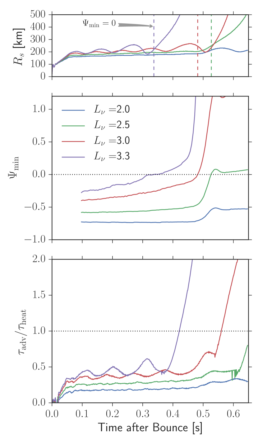
Figure 11: A comparison of the explosion diagnostic, $\Psi_{\rm min}>0$, and a timescale ratio condition, $\tau_{\rm adv}/\tau_{\rm heat}$. The top plot shows $\Psi_{\rm min}$ and the bottom plot shows the ratio of the advection time ($\tau_{\rm adv}$) to the heating time ($\tau_{\rm heat}$). The advection timescale is defined as $\tau_{\rm adv}=M_{\rm gain}/\dot{\mathcal{M}}$, where $M_{\rm gain}$ is the mass in between the gain radius and the shock. We adopt a heating timescale that is a ratio of energy and heating rate in the gain region: $\tau_{\rm heat}=E/Q_{\rm gain}$, where $Q_{\rm gain}=\int_{r_{\rm gain}}^{R_{s}}(H-C)\rho\,dV$, and $E=\int_{\rm gain}\varepsilon\rho\,dV$ is the total internal energy in the gain region. The $\tau_{\rm adv}/\tau_{\rm heat}$ is an approximate heuristic explosion diagnostic. The choice of the terms to define the timescales and the region over which to integrate are arbitrary. The timescale ratio is $\mathcal{O}(1)$ but it shows no sign of a reliable “critical” value or utility in predicting explosion. In fact, it is only as good as using the shock radius as an explosion diagnostic. On the other hand, $\Psi_{\rm min}$ works quite well as an explosion diagnostic.

The final comparison is between $\Psi_{\rm min}$ and the antesonic condition of Pejcha & Thompson (2012); see Figure 12. Similar to our motivation, Pejcha & Thompson (2012) were motivated to explain the origin of the critical luminosity curve and possibly derive a more general condition. They took a slightly different tack. Pejcha & Thompson (2012) considered the family of accretion and wind solutions and hypothesized that explosion occurs at the intersection between steady-state accretion solutions and steady-state wind solutions. By considering isothermal profiles, they were able to define an analytic condition that divides these solutions. For $c_{T}^{2}/v_{\rm esc}^{2}>3/16$, only wind solutions are possible, which they attributed to the transition between steady-state accretion and explosion. Given the great deal of neutrino heating and neutrino cooling, the post-shock profile is certainly not isothermal. Therefore, they were unable to derive a similar analytic condition in a more realistic CCSN context. Instead, they solved the steady-state equations and empirically searched for a similar condition that would be appropriate for the core-collapse case. The resulting explosion condition that they proposed is the antesonic condition, $\max(c_{s}/v_{\rm esc})^{2}\gtrsim 0.19$, where $\max()$ denotes the maximum in between the NS and the shock. Empirically, our one-dimensional simulations indicate that a value of $\sim$0.19 is about right. In multidimensional simulations, Müller et al. (2012a) and Burrows (2013) found a much higher value of $\sim$0.3. However, given that the antesonic condition was derived and discussed in the context of one-dimensional spherical symmetry, it is no surprise that the multidimensional simulations do not match. After all, we derive an integral condition in the same spherically symmetric context. In a forthcoming paper, we rederive the integral condition including turbulence, and find that the new integral condition is consistent with simulations. We suspect that one could do the same for the antesonic condition. However, to use the antesonic condition in practice, one must measure the “critical” condition in simulations ex post facto. While the antesonic condition, which is analytically derived in the isothermal case and empirically derived in the nonisothermal case, is imperfect, Figure 12 shows that it fairs a little better than the timescale ratio condition.

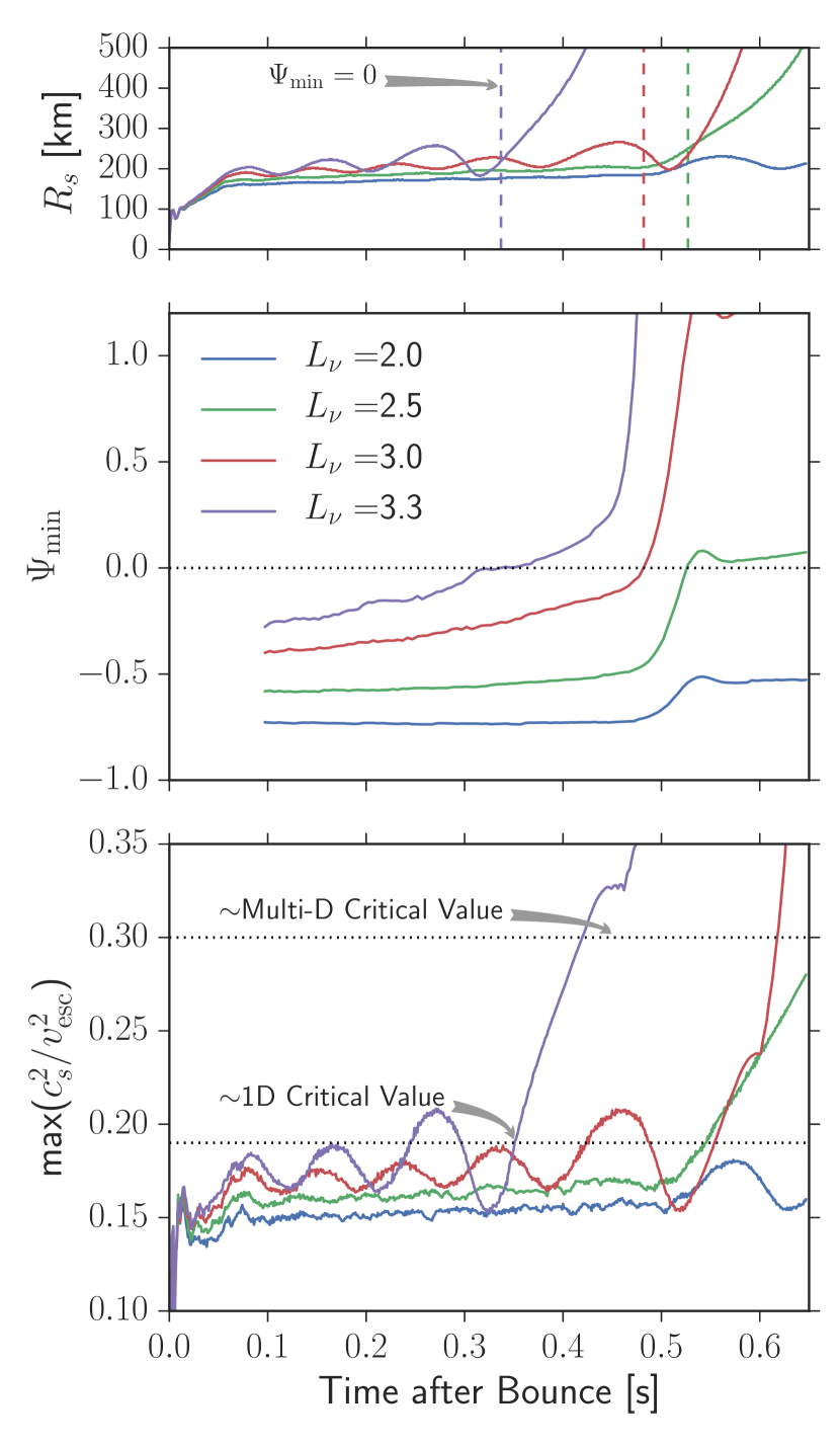
Figure 12: The $\Psi_{\rm min}$ explosion diagnostic in comparison with the antesonic condition of Pejcha & Thompson (2012). For an isothermal flow in one dimension, Pejcha & Thompson (2012) show that there are no steady-state accretion solutions that match the pre-shock flow for $c_{T}^{2}/v_{\rm esc}^{2}>3/16$. By analogy, they propose that a similar condition exists for the nonisothermal situation of the core-collapse problem. By numerically exploring the steady-state solutions in one-dimensional approximations, they propose that $\max(c_{s}^{2}/v_{\rm esc}^{2})\gtrsim 0.19$ divides steady-state accretion from explosion. In multidimensional simulations, Müller et al. (2012a) and Dolence et al. (2013) empirically find that $\max(c_{s}^{2}/v_{\rm esc}^{2})\gtrsim 0.3$ is a better “critical” value. The bottom panel of this figure shows that the one-dimensional “critical” value is a decent indicator of explosion. It certainly performs better than the timescale ratio seen in Figure 11. Still, the $\Psi_{\rm min}>0$ condition has some practical advantages. For one, $\Psi_{\rm min}>0$ is an integral condition derived from the supposition that $v_{s}>0$ corresponds to explosion. Second, the dynamic range of $\Psi_{\rm min}$ illustrates more clearly which simulations are far from explosion. Third, while the lowest luminosity model appears to always approach explosion for the $\max(c_{s}^{2}/v_{\rm esc}^{2})$ condition, the $\Psi_{\rm min}$ condition clearly shows that the $L_{\nu}=2.0$ model moves away from explosion, except when the density shelf accretes through the shock, but then again it moves away from explosion. Fourth, $\max(c_{s}^{2}/v_{\rm esc}^{2})\gtrsim 0.19$ does not predict explosion: the actual antesonic condition overshoots the proposed critical value by 10% before it actually explodes, which is half of the full dynamic range of the antesonic condition ($\sim 20$%); when the antesonic condition looks as if it indicates explosion, it does so well after the initiation of explosion.

While the antesonic condition fares slightly better than the timescale ratio at predicting explosion, it still remains less favorable compared to the integral condition (middle panel of Figure 12). For one, like the timescale ratio, the dramatic upward trend in the antesonic ratio that might be attributed to explosion actually occurs well after explosion; this means that one can rule out using the upward trend as an explosion diagnostic. One of the useful features of the integral condition, $\Psi_{\rm min}>0$ is that one can tell even before explosion that a model is unlikely to explode. There are two features that enable this: 1) the closeness of $\Psi_{\rm min}$ to zero, and 2) the trend toward or away from zero; for example, $\Psi_{\rm min}$ for the $L_{\nu}=3.0$ model marches toward explosion, while $\Psi_{\rm min}$ for the $L_{\nu}=2.0$ model marches away from explosion. Similar to point 1) for the integral condition, the antesonic condition is indeed closer to the “critical” value before explosion. However, even the antesonic diagnostic for the $L_{\nu}=2.0$ marches toward the “critical” value even though it never explodes. Furthermore, the antesonic diagnostic overshoots the “critical” value by $\sim$10% of the “critical” value. This may seem like a triumph of estimating the “critical” value, but the dynamic range of the antesonic diagnostic is only $\sim$20% of the “critical” value, making the estimate only $\sim$50% accurate when considering the dynamic range of the antesonic diagnostic.

7 Discussion and Conclusions

For many years, the critical neutrino luminosity curve has been the most impactful model for understanding successful explosion conditions. However, no one had demonstrated analytically that the solutions above the curve are explosive, nor had anyone successfully used the critical neutrino luminosity as an explosion diagnostic for core-collapse simulations. In this manuscript, we took steps to show that the solutions above the critical neutrino luminosity have $v_{s}>0$, and we used this derivation to propose an explosion diagnostic for core-collapse simulations. When we began this project, our primary goal was to merely show that the solutions above the critical neutrino luminosity curve are explosive. We have partially done so by deriving an integral condition, $\Psi_{\rm min}\geq 0$, for $v_{s}\geq 0$ and showing that the solutions above the critical neutrino luminosity curve have $v_{s}>0$. Along the way to deriving this integral condition, we discovered that the neutrino luminosity curve is a projection of a more general critical hypersurface. Most strikingly, this critical hypersurface is represented by a single dimensionless parameter, $\Psi_{\rm min}\geq 0$, and it promises to be a useful explosion diagnostic for core-collapse simulations.

In deriving the integral condition $\Psi\geq 0$, we made two simple but profound approximations: (1) we considered steady-state solutions, and (2) we considered that $v_{s}>0$ corresponds to explosion. With these two approximations, we derived an integral condition for $v_{s}\geq 0$ and recast it in a dimensionless form, $\Psi\geq 0$. We verified this integral condition using one-dimensional parameterized simulations and found that during the stalled-shock phase $\Psi\approx 0$ and during explosion $\Psi>0$. Although the comparisons with simulations successfully verified the integral condition, they also demonstrated that simply calculating $\Psi$ from the simulations is not a useful explosion diagnostic. Because the simulations always find a stalled-shock solution before explosion, $\Psi$ is always zero before explosion. Such a diagnostic fails to indicate a distance to explosion. If, on the other hand, we extract the important parameters from the simulations and calculate all of the possible steady-state solutions, then a better diagnostic emerges.

The steady-state solutions fall into one of two broad categories: in one category, a stalled-shock solution exists, and in the other, only $v_{s}>0$ solutions exist. To understand the origin of these categories, one must first understand that there are five important parameters that characterize each steady-state solution: $L_{\nu}$ (neutrino luminosity), $T_{\nu}$ (neutrino temperature), $R_{\nu}$ (neutrino-sphere radius or proto-neutron star radius), $M_{\rm NS}$ (proto-neutron star mass), and $\dot{M}$ (accretion rate). For a fixed set of parameters, there is a family of solutions, and each solution in this family has a different value of $\Psi$. In general, $\Psi$ may be negative, zero, or positive, and because $\Psi\propto v_{s}$, each solution may have $v_{s}<0$, $v_{s}=0$, or $v_{s}>0$. If a $v_{s}=0$ solutions exists, it represents the preferred quasi-equilibrium solution. Generically, for each family of solutions, there is a minimum $\Psi$ that we denote $\Psi_{\rm min}$, and it is this parameter that determines whether a solution belongs to the stalled-shock category or to the explosive category. If $\Psi_{\rm min}<0$, then the family of solutions has solutions with $v_{s}<0$, $v_{s}=0$, and $v_{s}>0$ with the $v_{s}=0$ being the preferred quasi-equilibrium solution. If on the other hand, $\Psi_{\rm min}>0$, then only $v_{s}>0$ solutions exist. If we attribute $v_{s}>0$ to explosions, then $\Psi_{\rm min}$ is a useful explosion diagnostic.

We calculated $\Psi_{\rm min}$ for several one-dimensional parameterized simulations (see Figure 8) and find that the time evolution of $\Psi_{\rm min}$ makes an excellent explosion diagnostic. From the time that we track $\Psi_{\rm min}$, one can tell whether a simulation is near explosion. For those that are near explosion, $\Psi_{\rm min}$ tends to march toward explosion throughout much of the simulation. The model that does not explode shows a general evolution of $\Psi_{\rm min}$ away from explosion. Next, we need to explore $\Psi_{\rm min}$ in the context of multidimensional and self-consistent neutrino radiation hydrodynamic simulations to see if these promising behaviors remain.

In section 6 and Figures 11 & 12, we compared this new integral condition with explosion conditions that have been defined previously. Specifically, we compared $\Psi_{\rm min}>0$ to a timescale ratio condition and the antesonic condition. In contrast to the integral condition, the $\tau_{\rm adv}/\tau_{\rm heat}$ condition is heuristic, only good to order unity, shows no obvious “critical” value, and is no better than simply using $R_{s}$ as an explosion diagnostic. The antesonic condition fares better than the timescale ratio condition. Even so, it lacks the accuracy and predictive attributes of the integral condition.

To derive the integral condition, we made two approximations that must be investigated further: we assumed that $v_{s}>0$ corresponds to explosion, and we assumed steady-state throughout our derivation. These are two very strong assumptions that could have invalidated our derivation. For example, $v_{s}>0$ does not necessarily equate to explosion, especially when we relax the steady-state condition. Oscillations of the shock are one example in which $v_{s}>0$ may manifest but not lead to explosion. In order to make progress, we decided to see where these approximations led. In the end, we were able to derive an integral explosion diagnostic that successfully describes the explosion conditions of parameterized one-dimensional simulations. However, we did not show that once $\Psi_{\rm min}>0$ and the shock begins to move outward that it continues to move outward. In some sense, one expects the shock to continue to move out, because once $\Psi_{\rm min}>0$ the only steady-state solutions are solutions with $v_{s}>0$, but this does not preclude the possibility of a dynamic (non-steady-state) solution that is oscillatory. A next step in confirming our derivation is to show that once $\Psi_{\rm min}>0$, the dynamic solution is a solution in which $v_{s}>0$ continues.

We found the integral condition to be a successful explosion diagnostic for one-dimensional parameterized explosions, but we suspect that it can do much more. We suspect that the integral condition may be an excellent explosion diagnostic for self-consistent three-dimensional CCSN simulations. One may even be able to predict whether a certain progenitor model will explode without even performing core-collapse simulations. This hope will only be realized with further model developments, replacing parameters currently measured from simulations with parameters calculated by other means.

Before we can even pursue such bold endeavors, however, we must adapt the integral condition to include the appropriate physics. For one, we derived the integral condition using Newtonian gravity; general relativistic considerations are important, therefore we will need to take the straightforward steps in deriving the condition in GR. Second, we need to incorporate a more self-consistent neutrino heating and cooling. Third, we need to incorporate multidimensional effects. Turbulence seems to reduce the critical neutrino luminosity for explosion; we suspect that one can easily use a turbulence model to derive a new integral condition for explosion including turbulence.

In summary, we derived an integral condition for explosion and verified it with one-dimensional parameterized simulations. When combined with simple steady-state models, it suggests a new explosion diagnostic, $\Psi_{\rm min}$, that we argue may be a more predictive measure of a models explodability than other diagnostics. Finally, we point out that our integral formulation can be extended with better physics, and we are hopeful that this approach may prove useful in disentangling the complicated interactions of various physical effects and in understanding the mechanism of CCSNe in Nature.

Appendix A Steady-State Equations

Identifying the steady-state solution with the minimum $\Psi$ is key in developing the explosion diagnostic in section 5 and Figure 8. In this appendix, we therefore present the steady-state equations that we used to obtain the family of solutions.

To accommodate the analytic EOS described in the next appendix, we recast the steady-state equations in terms of the natural independent variables. Because the analytic EOS in appendix B is most naturally written as a function of density and temperature, $P=P(\rho,T)$, we rewrite the steady-state equations as differential equations for $v$, $\rho$, and $T$.

$$\frac{d\ln v}{d\ln r}=-\left(2+\frac{d\ln\rho}{d\ln r}\right)\,$$ (A1)

$$\frac{d\ln\rho}{d\ln r}\left(yP_{\rho}-\frac{v^{2}}{\phi}\right)=-yP_{T}\frac{d\ln T}{d\ln r}-1+\frac{2v^{2}}{\phi}\,$$ (A2)

and

$$e_{T}\frac{d\ln T}{d\ln r}=(\gamma_{4}-1-e_{\rho})\frac{d\ln\rho}{d\ln r}-\frac{L_{\nu}\kappa\rho r}{\dot{\mathcal{M}}\varepsilon}+\frac{\rho C_{0}(T/T_{0})^{6}}{\dot{\mathcal{M}}\varepsilon}\,,$$ (A3)

where $P_{\rho}=(\partial\ln P/\partial\ln\rho)_{T}$ is the partial derivative of $P$ with respect to $\rho$ at constant $T$. Equivalently, $P_{T}=(\partial\ln P/\partial\ln T)_{\rho}$, $e_{\rho}=(\partial\ln\varepsilon/\partial\ln\rho)_{T}$, and $e_{T}=(\partial\ln\varepsilon/\partial\ln T)_{\rho}$.

Appendix B Equation of State

For the one-dimensional parameterized simulations, we use the tabulated EOS provided by Hempel et al. (2012). The microphysics includes a distribution of nuclei that satisfy nuclear statistical equilibrium; the individual components are, broadly, a dense nuclear component, ideal gas for the nucleons and isotopes, photon gas, and relativistic electrons and positrons with arbitrary degeneracy. The tabulated EOS and driver are available at http://www.stellarcollapse.org/equationofstate.

For the steady-state solutions we use an analytic EOS that does remarkably well in reproducing the microphysics in the region between the neutrino sphere and the shock. Bethe (1990), Janka (2001), and Fernández & Thompson (2009) were useful guides in developing this analytic EOS. First, we assume nuclear statistical equilibrium for three species only: neutrons, protons, and $\alpha$s; their respective mass fractions are $X_{n}$, $X_{p}$, and $X_{\alpha}$. Conservation of baryonic mass implies

$$X_{n}+X_{p}+X_{\alpha}=1\,,$$ (B1)

and conservation of charge implies

$$X_{p}+\frac{1}{2}X_{\alpha}=Y_{e}\,$$ (B2)

where $Y_{e}$ is the number of electrons per baryon. In our steady-state solutions we simply set $Y_{e}=0.5$. In NSE, the Saha equation provides the remaining equation to find a solution for the abundance of these three species.

$$X_{n}^{2}X_{p}^{2}=\frac{1}{2}X_{\alpha}\left(\frac{m_{p}n_{q}}{\rho}\right)^{3}\exp(\frac{-Q_{\alpha}}{k_{B}T})\,,$$ (B3)

with

$$n_{q}=\left(\frac{m_{p}k_{B}T}{2\pi\hbar^{2}}\right)^{3/2}\,,$$ (B4)

and $Q_{\alpha}=28$ MeV is the binding energy of the $\alpha$.

We construct the pressure and internal energy under the assumptions that the photons, positrons, and electrons are relativistic and the partial pressure due to the nucleons and $\alpha$s is given by the ideal gas law. In addition, we consider the electrons and positrons with an arbitrary degeneracy $\eta=\mu_{e}/(k_{B}T)$. The expression for the degeneracy parameter is

$$\rho=\frac{m_{u}}{3\pi^{2}Y_{e}}\left(\frac{k_{B}T}{\hbar c}\right)^{3}\eta(\pi^{2}+\eta^{2})\,.$$ (B5)

The pressure and internal energy may both be divided into partial pressures due to relativistic ($R$) particles and nonrelativistic ($NR$) particles

$$P=P_{R}+P_{NR}\,,$$ (B6)

and

$$\varepsilon=\varepsilon_{R}+\varepsilon_{NR}\,.$$ (B7)

The partial pressure due to the relativistic constituents is

$$P_{R}=\frac{1}{12}\frac{(k_{B}T)^{4}}{(\hbar c)^{3}}\left(\frac{11\pi^{2}}{15}+2\eta^{2}+\frac{\eta^{4}}{\pi^{2}}\right)\,,$$ (B8)

and the partial pressure due to the nonrelativistic constituents is

$$P_{NR}=\left(1-\frac{3}{4}X_{\alpha}\right)\frac{\rho k_{B}T}{m_{u}}\,.$$ (B9)

The resulting internal energy is

$$\varepsilon=3\frac{P}{\rho}-\frac{3}{2}\frac{P_{NR}}{\rho}+(1-X_{\alpha})\frac{Q_{\alpha}}{4}\,,$$ (B10)

where the last term is there to account for the transfer of binding energy per nucleon from $X_{\alpha}$ to the gas.

References

- Bethe (1990) Bethe, H. A. 1990, Reviews of Modern Physics, 62, 801
- Bethe & Wilson (1985) Bethe, H. A., & Wilson, J. R. 1985, ApJ, 295, 14
- Bruenn et al. (2016) Bruenn, S. W., Lentz, E. J., Hix, W. R., et al. 2016, ApJ, 818, 123
- Buras et al. (2006a) Buras, R., Janka, H.-T., Rampp, M., & Kifonidis, K. 2006a, A&A, 457, 281
- Buras et al. (2003) Buras, R., Rampp, M., Janka, H.-T., & Kifonidis, K. 2003, Physical Review Letters, 90, 241101
- Buras et al. (2006b) —. 2006b, A&A, 447, 1049
- Burrows (2013) Burrows, A. 2013, Reviews of Modern Physics, 85, 245
- Burrows et al. (2007) Burrows, A., Dessart, L., & Livne, E. 2007, in American Institute of Physics Conference Series, Vol. 937, Supernova 1987A: 20 Years After: Supernovae and Gamma-Ray Bursters, ed. S. Immler & R. McCray, 370–380
- Burrows & Goshy (1993) Burrows, A., & Goshy, J. 1993, ApJ, 416, L75
- Burrows et al. (1995) Burrows, A., Hayes, J., & Fryxell, B. A. 1995, ApJ, 450, 830
- Colgate & White (1966) Colgate, S. A., & White, R. H. 1966, ApJ, 143, 626
- Couch (2012) Couch, S. M. 2012, ArXiv e-prints, arXiv:1206.4724
- Couch (2013) —. 2013, ApJ, 775, 35
- Dolence et al. (2013) Dolence, J. C., Burrows, A., Murphy, J. W., & Nordhaus, J. 2013, ApJ, 765, 110
- Dolence et al. (2015) Dolence, J. C., Burrows, A., & Zhang, W. 2015, ApJ, 800, 10
- Fernández (2012) Fernández, R. 2012, ApJ, 749, 142
- Fernández & Thompson (2009) Fernández, R., & Thompson, C. 2009, ApJ, 703, 1464
- Fischer et al. (2009) Fischer, T., Whitehouse, S. C., Mezzacappa, A., Thielemann, F.-K., & Liebendörfer, M. 2009, A&A, 499, 1
- Fryer et al. (2012) Fryer, C. L., Belczynski, K., Wiktorowicz, G., et al. 2012, ApJ, 749, 91
- Hanke et al. (2012) Hanke, F., Marek, A., Müller, B., & Janka, H.-T. 2012, ApJ, 755, 138
- Hanke et al. (2013) Hanke, F., Müller, B., Wongwathanarat, A., Marek, A., & Janka, H.-T. 2013, ApJ, 770, 66
- Hempel et al. (2012) Hempel, M., Fischer, T., Schaffner-Bielich, J., & Liebendörfer, M. 2012, ApJ, 748, 70
- Herant et al. (1994) Herant, M., Benz, W., Hix, W. R., Fryer, C. L., & Colgate, S. A. 1994, ApJ, 435, 339
- Hillebrandt & Mueller (1981) Hillebrandt, W., & Mueller, E. 1981, A&A, 103, 147
- Horiuchi et al. (2011) Horiuchi, S., Beacom, J. F., Kochanek, C. S., et al. 2011, ApJ, 738, 154
- Janka (2001) Janka, H.-T. 2001, A&A, 368, 527
- Janka (2012) —. 2012, Annual Review of Nuclear and Particle Science, 62, 407
- Janka & Keil (1998) Janka, H.-T., & Keil, W. 1998, in Supernovae and cosmology, ed. L. Labhardt, B. Binggeli, & R. Buser, 7
- Janka & Müller (1995) Janka, H.-T., & Müller, E. 1995, ApJ, 448, L109
- Janka & Müller (1996) —. 1996, A&A, 306, 167
- Lattimer & Prakash (2016) Lattimer, J. M., & Prakash, M. 2016, Phys. Rep., 621, 127
- Lentz et al. (2015) Lentz, E. J., Bruenn, S. W., Hix, W. R., et al. 2015, ArXiv e-prints, arXiv:1505.05110
- Li et al. (2010) Li, W., Leaman, J., Chornock, R., et al. 2010, ArXiv e-prints, arXiv:1006.4612
- Liebendörfer et al. (2001a) Liebendörfer, M., Mezzacappa, A., & Thielemann, F.-K. 2001a, Phys. Rev. D, 63, 104003
- Liebendörfer et al. (2001b) Liebendörfer, M., Mezzacappa, A., Thielemann, F.-K., et al. 2001b, Phys. Rev. D, 63, 103004
- Liebendörfer et al. (2005) Liebendörfer, M., Rampp, M., Janka, H.-T., & Mezzacappa, A. 2005, ApJ, 620, 840
- Mabanta et al. (in prep. 2017) Mabanta, Q., Murphy, J. W., & Dolence, J. C. in prep. 2017
- Mazurek (1982) Mazurek, T. J. 1982, ApJ, 259, L13
- Mazurek et al. (1982) Mazurek, T. J., Cooperstein, J., & Kahana, S. 1982, in NATO Advanced Science Institutes (ASI) Series C, Vol. 90, NATO Advanced Science Institutes (ASI) Series C, ed. M. J. Rees & R. J. Stoneham, 71–77
- Melson et al. (2015) Melson, T., Janka, H.-T., & Marek, A. 2015, ApJ, 801, L24
- Müller et al. (2012a) Müller, B., Janka, H.-T., & Heger, A. 2012a, ApJ, 761, 72
- Müller et al. (2012b) Müller, B., Janka, H.-T., & Marek, A. 2012b, ApJ, 756, 84
- Murphy & Bloor (in prep. 2017) Murphy, J. W., & Bloor, E. in prep. 2017
- Murphy & Burrows (2008) Murphy, J. W., & Burrows, A. 2008, ApJ, 688, 1159
- Murphy et al. (2013) Murphy, J. W., Dolence, J. C., & Burrows, A. 2013, ApJ, 771, 52
- Murphy & Meakin (2011) Murphy, J. W., & Meakin, C. 2011, ApJ, 742, 74
- O’Connor & Ott (2011) O’Connor, E., & Ott, C. D. 2011, ApJ, 730, 70
- Ohnishi et al. (2006) Ohnishi, N., Kotake, K., & Yamada, S. 2006, ApJ, 641, 1018
- Ott et al. (2008) Ott, C. D., Burrows, A., Dessart, L., & Livne, E. 2008, ApJ, 685, 1069
- Pejcha & Thompson (2012) Pejcha, O., & Thompson, T. A. 2012, ApJ, 746, 106
- Rampp & Janka (2002) Rampp, M., & Janka, H.-T. 2002, A&A, 396, 361
- Roberts et al. (2016) Roberts, L. F., Ott, C. D., Haas, R., et al. 2016, ArXiv e-prints, arXiv:1604.07848
- Suwa et al. (2014) Suwa, Y., Yamada, S., Takiwaki, T., & Kotake, K. 2014, ArXiv e-prints, arXiv:1406.6414
- Takiwaki et al. (2014) Takiwaki, T., Kotake, K., & Suwa, Y. 2014, ApJ, 786, 83
- Thompson (2000) Thompson, C. 2000, ApJ, 534, 915
- Thompson et al. (2003) Thompson, T. A., Burrows, A., & Pinto, P. A. 2003, ApJ, 592, 434
- Thompson et al. (2005) Thompson, T. A., Quataert, E., & Burrows, A. 2005, ApJ, 620, 861
- Woosley & Heger (2007) Woosley, S. E., & Heger, A. 2007, Phys. Rep., 442, 269
- Yamasaki & Foglizzo (2008) Yamasaki, T., & Foglizzo, T. 2008, ApJ, 679, 607
- Yamasaki & Yamada (2005) Yamasaki, T., & Yamada, S. 2005, ApJ, 623, 1000
- Yamasaki & Yamada (2006) —. 2006, ApJ, 650, 291