Exponential Bounds for the Hypergeometric Distribution

Abstract

We establish exponential bounds for the hypergeometric distribution which include a finite sampling correction factor, but are otherwise analogous to bounds for the binomial distribution due to León and Perron (2003) and Talagrand (1994). We also extend a convex ordering of Kemperman’s (1973) for sampling without replacement from populations of real numbers between zero and one: a population of all zeros or ones (and hence yielding a hypergeometric distribution in the upper bound) gives the extreme case.

and label=u1,url]http://www.stat.washington.edu/jaw/

t1Supported in part by NSF Grant DMS-1104832 t2Supported in part by NSF Grant DMS-1104832 and NI-AID grant 2R01 AI291968-04

1 Introduction and overview

In this paper we derive several exponential bounds for the tail of the hypergeometric distribution. This distribution emerges as an extreme case in the setting of sampling without replacement from a finite population. We begin with a description of this setting. Consider a population $C$ containing $N$ elements, $C:=\left\{c_{1},\dots,c_{N}\right\}$, with $c_{i}\in\mathbb{R}$. Let $N=|C|$ denote the cardinality of this set, $a$ the value of the minimum element, $b$ the value of the maximum element, and $\mu:=(N^{-1})(\sum_{i=1}^{N}c_{i})$, the population mean. Let $1\leq i\leq n\leq N$, and $X_{i}$ denote the $i^{th}$ draw without replacement from this population. Finally, let $S_{n}:=\sum_{i=1}^{n}X_{i}$ denote the sum of this sampling procedure, and let $\bar{X}_{n}:=S_{n}/n$ denote the sample mean.

R. J. Serfling obtained the following bound.

Finite Sampling Bound 1.

(Serfling [19]) For $1\leq n\leq N$, $S_{n}$ the sum in sampling without replacement, and $\lambda>0$:

$$P\left(\sqrt{n}(\bar{X}_{n}-\mu)\geq\lambda\right)\leq\exp\left(-\frac{2\lambda^{2}}{(1-f_{n}^{*})(b-a)^{2}}\right)$$ (1.1)

where $f_{n}^{*}:=(n-1)/N$.

This result applies to sampling without replacement from any finite bounded population. Let $D,N\in\mathbb{N}$ such that $D<N$. Then as a special case we may apply the bound to a population of $N$ elements containing $D$ $1$’s and $N-D$ $0$’s. Note that in this specific case $S_{n}=:S_{n,D,N}\sim\text{Hypergeometric}(n,D,N)$.

For the hypergeometric distribution, the following facts are well known:

$$P(S_{n}=k) = \frac{{D\choose k}{N-D\choose n-k}}{{N\choose n}},\ \ \ \max\{0,n-(N-D)\}\leq k\leq\min\{D,n\},$$

$$E(S_{n}) = n\left(\frac{D}{N}\right),$$

$$Var(S_{n}) = n\left(\frac{D}{N}\right)\left(1-\frac{D}{N}\right)\left(1-\frac{n-1}{N-1}\right)=:n\mu_{D,N}(1-\mu_{D,N})(1-f_{n})$$ (1.2)

with the final line defining $\mu_{D,N}:=D/N$ and $f_{n}:=(n-1)/(N-1)$. Applying Serfling’s result to the case of the hypergeometric distribution immediately gives

$$P\left(\sqrt{n}(\bar{X}_{n}-\mu_{D,N})\geq\lambda\right)\leq\exp\left(-\frac{2\lambda^{2}}{(1-f_{n}^{*})}\right)$$ (1.3)

since $(b-a)^{2}=(1-0)^{2}=1$. Comparison of the factor $1-f_{n}^{*}$ in Serfling’s bound to the factor $1-f_{n}$ in (1.2) suggests the following question: can Serfling’s bound be improved to

$$P\left(\sqrt{n}(\bar{X}_{n}-\mu)\geq\lambda\right)\leq\exp\left(-\frac{2\lambda^{2}}{(1-f_{n})(b-a)^{2}}\right)$$ (1.4)

in general, or at least in the special case of the hypergeometric distribution?

To date, the improvement conjectured in (1.4) has not been obtained. For the special case of the hypergeometric, Hush and Scovel derived the following bound by extending an argument given by Vapnik. See [12] and [23].

Hypergeometric Bound 1.

(Hush and Scovel, [12]) Suppose $S_{n}\sim\text{Hypergeometric(n,D,N)}$. Then for all $\lambda>0$ we have

$$P\left(\sqrt{n}(\bar{X}_{n}-\mu_{D,N})\geq\lambda\right)\leq\exp\left(-2\alpha_{n,D,N}(n\lambda^{2}-1)\right)$$ (1.5)

where

$$\alpha_{n,D,N}:=\left(\frac{1}{n+1}+\frac{1}{N-n+1}\right)\vee\left(\frac{1}{D+1}+\frac{1}{N-D+1}\right)\ .$$

More recently, Bardenet and Maillard have improved a deficiency in Serfling’s inequality that occurs when more than half the population is sampled without replacement by using a reverse-martingale argument. The statement here is a specialization of their Theorem 2.4 to the hypergeometric case. See [1] for additional discussion.

Hypergeometric Bound 2.

(Bardenet and Maillard [1]) Suppose $S_{n}\sim\text{Hypergeometric(n,D,N)}$. Then for all $\lambda>0$ and $n<N$ we have

$$P\left(\sqrt{n}(\bar{X}_{n}-\mu_{D,N})\geq\lambda\right)\leq\exp\left(-\frac{2\lambda^{2}}{(1-n/N)(1+1/n)}\right)\ .$$

We will justify the special consideration given to the hypergeometric distribution relative to the goal of obtaining (1.4) by adapting a result of Kemperman [14] to derive a convex order between samples without replacement from populations consisting of elements in $[0,1]$ and the hypergeometric distribution. We will then demonstrate how one may use this convex order to obtain exponential bounds for the more general problem of sampling without replacement from a bounded, finite population. In doing so, we return to the setting of Serfling. In this setting we will consider the variance of the population as well. Anticipating this, we conclude the introduction with a specialization of a bound of Bardenet and Maillard which incorporates information about the population variance into the bound.

Finite Sampling Bound 2.

(Bardenet and Maillard [1]) For $1\leq n<N$, $S_{n}$ the sum in sampling without replacement from a population $\mathbb{c}:=\left\{c_{1},\dots,c_{N}\right\}$, $\delta\in[0,1]$, and $\lambda>0$, we have

$$P\left(\sqrt{n}(\bar{X}_{n}-\mu)\geq\lambda\right)\leq\exp\left(-\frac{\lambda^{2}}{2(\gamma^{2}+(2/3)(b-a)(\lambda/\sqrt{n}))}\right)+\delta$$ (1.6)

where

$$a :=\min_{1\leq i\leq N}c_{i}\ ,\ b:=\max_{1\leq i\leq N}c_{i}\ ,\ f_{n}^{*}:=(n-1)/N\ ,\ \mu:=(1/N)\sum_{i=1}^{N}c_{i}\ ,\ \sigma^{2}:=(1/N)\sum_{i=1}^{N}(c_{i}-\mu)^{2}\ ,$$

$$\gamma^{2} :=(1-f_{n}^{*})\sigma^{2}+f_{n}^{*}c_{n-1}(\delta)\ ,\text{ and }\ c_{n}(\delta):=\sigma(b-a)\sqrt{\frac{2\log(1/\delta)}{n}}\ .$$

2 Exponential Bounds

Binomial distributions arise when sampling with replacement from a population consisting only of $0$’s and $1$’s. As we saw in the introduction, hypergeometric distributions arise when sampling without replacement from such populations. Intuitively, sampling without replacement is more informative than sampling with replacement: when items are not replaced, eventually, when $n=N$, the entire population is sampled. This being the case, it is natural to guess that upper bounds which apply to binomial tail probabilities will also apply to the hypergeometric tail probabilities.

Hoeffding [10] proved that this guess is true for exponential bounds derived via the Cramér - Chernoff method. This is because a convex order exists between samples with and without replacement (Hoeffding proves this order in his Theorem 4). Convex orders between a variety of sampling plans were subsequently explored by Kemperman [14] and Karlin [13].

Note that by Ehm (Theorem 2 [4]; see also Holmes, Theorem 3.2 [11]), the total variation distance between the hypergeometric distribution $P_{n,D,N}^{hyper}$ and the binomial distribution $P_{n,D/N}^{bin}$ satisfies

$$d_{TV}(P_{n,D,N}^{hyper},P_{n,D/N}^{bin})\leq\frac{n}{n+1}(1-(D/N)^{n+1}-(1-D/N)^{n+1})\frac{n-1}{N-1}\leq\frac{n-1}{N-1},$$

so we expect that the binomial bounds will be essentially optimal when $(n-1)/(N-1)\rightarrow 0$.

Here we are interested in sampling scenarios in which $(n-1)/(N-1)\not\rightarrow 0$. Given the similarity in scenarios that produce binomial and hypergeometric probabilities, one might expect that the binomial exponential bounds provide a clue to the form that hypergeometric exponential bounds will take: hypergeometric bounds look like binomial bounds, with a finite sampling correction factor included. Indeed, this is the case when we compare the bound of Serfling (1.1) to Hoeffding’s uniform bound (Theorem 2.1 [10]), since the only difference between the two is the quantity $1-f_{n}^{*}$. We therefore state several exponential bounds which apply to the binomial distribution.

Binomial Bound 1.

(León and Perron [15]) Let $n\geq 1$, $p\in(0,1)$, $\lambda<\sqrt{n}/2$, and $X_{1},\dots,X_{n}$ be independent Bernoulli$(p)$ random variables. Then

$$P(\sqrt{n}(\bar{X}_{n}-p)\geq\lambda)\leq\sqrt{\frac{1}{2\pi\lambda^{2}}}\left(\frac{1}{2}\right)\sqrt{\frac{\sqrt{n}+2\lambda}{\sqrt{n}-2\lambda}}e^{-\left(2\lambda^{2}\right)}\ .$$ (2.1)

The second bound was established by Talagrand [21, pp. 48–50]. The statement here is taken from van der Vaart and Wellner [22, pp. 460–462]):

Binomial Bound 2.

(Talagrand [21]) Fix $p_{0}$ and consider $p$ such that $0<p_{0}\leq p\leq 1-p_{0}<1$. Suppose for $n\in\mathbb{N}$ that $X_{1},\dots,X_{n}$ are i.i.d. Bernoulli$(p)$ random variables. Then there exist constants $K_{1}$ and $K_{2}$ depending only on $p_{0}$, such that:

$$(i)\ \text{For all }\lambda>0,\ \ \ P\left(\sqrt{n}(\bar{X}_{n}-p)=\lambda\right)\leq\frac{K_{1}}{\sqrt{n}}\exp\left(-\left[2\lambda^{2}+\frac{\lambda^{4}}{4n}\right]\right)\ .$$

$$(ii)\ \text{For all }0<t<\lambda,\ \ \ P\left(\sqrt{n}(\bar{X}_{n}-p)\geq t\right)\leq\frac{K_{2}}{\lambda}\exp\left(-\left[2\lambda^{2}+\frac{\lambda^{4}}{4n}\right]\right)\exp\left(5\lambda[\lambda-t]\right)\ .$$

$$(iii)\ \text{For all }\lambda>0,\ \ \ P\left(\sqrt{n}(\bar{X}_{n}-p)\geq\lambda\right)\leq\frac{K_{2}}{\lambda}\exp\left(-\left[2\lambda^{2}+\frac{\lambda^{4}}{4n}\right]\right)\ .$$ (2.2)

Another well-known exponential bound which applies to sums of independent random variables (and consequently the binomial distribution) was discovered by Bennett [2]. Bennett’s bound incorporates information about the population variance, and so obtains notable improvements when the population variance is small. This statement of Bennett’s inequality specialized to the binomial setting is adapted from Shorack and Wellner [20].

Binomial Bound 3.

(Bennett [2]) Let $X_{1},\dots,X_{n}$ i.i.d. $\text{Bernoulli}(\mu)$, with $0<\mu\leq 1/2$. Then for all $\lambda\geq 0$

$$P(\sqrt{n}(\bar{X}_{n}-\mu)\geq\lambda)\leq\exp\left(-\frac{\lambda^{2}}{2\mu(1-\mu)}\psi\left(\frac{\lambda}{\sqrt{n}\mu(1-\mu)}\right)\right)$$ (2.3)

where $\psi(\lambda):=(2/\lambda^{2})h(1+\lambda)$ where $h(\lambda):=\lambda(\log\lambda-1)+1$.

Inspecting the form of (2.1), (2.2), and (2.3), we notice that when these bounds are compared to the hypergeometric tail bound (1.3) obtained from Serfling’s bound they do not take advantage of the finite sampling setting. Our hope then is we can derive probability bounds which look like the preceding binomial expressions, but improved by a finite-sampling correction factor. Such improved bounds exist and are the main results of this paper. Their statements follow.

Theorem 1.

Suppose $S_{n}\sim Hypergeometric(n,D,N)$. Define $\mu:=D/N$, and suppose $N>4$ and $2\leq n<D\leq N/2$. Then for all $0<\lambda<\sqrt{n}/2$ we have

$$P\left(\sqrt{n}(\bar{X}_{n}-\mu)\geq\lambda\right)\leq \sqrt{\frac{1}{2\pi\lambda^{2}}}\left(\frac{1}{2}\right)\sqrt{\left(\frac{N-n}{N}\right)\left(\frac{\sqrt{n}+2\lambda}{\sqrt{n}-2\lambda}\right)\left(\frac{N-n+2\sqrt{n}\lambda}{N-n-2\sqrt{n}\lambda}\right)}$$

$$\cdot\ \ \exp\left(-\frac{2}{1-\frac{n}{N}}\lambda^{2}\right)\exp\left(-\frac{1}{3}\left(1+\frac{n^{3}}{(N-n)^{3}}\right)\frac{\lambda^{4}}{n}\right)\ .$$ (2.4)

Theorem 2.

Suppose $\sum_{i=1}^{n}X_{i}\sim Hypergeometric(n,D,N)$. Define $\psi:=n/N$ and $\mu:=D/N$, and let $n<D$. Fix $\mu_{0},\psi_{0}>0$ such that $0<\mu_{0}\leq\mu\leq 1-\mu_{0}<1$ and $0<\psi_{0}\leq\psi\leq 1-\psi_{0}<1$. Then there exist constants $K_{1},K_{2}$ depending only on $\mu_{0}$ and $\psi_{0}$ such that:

$$(i)\ \text{For all }\lambda>0,\ \ \ P(\sqrt{n}(\overline{X}_{n}-\mu)=\lambda)\leq\frac{K_{1}}{\sqrt{n}}\exp\left(-\frac{2\lambda^{2}}{1-\frac{n}{N}}\right)\exp\left(-\left(\frac{1}{4}+\frac{1}{3}\left(\frac{n}{N-n}\right)^{3}\right)\frac{\lambda^{4}}{n}\right)\ .$$

$$(ii)\ \text{For all }0<t<\lambda,\ \ \ P(\sqrt{n}(\overline{X}_{n}-\mu)\geq t)\leq\frac{K_{2}}{\lambda}\begin{pmatrix}\exp\left(-\frac{2\lambda^{2}}{1-\frac{n}{N}}\right)\exp\left(-\left(\frac{1}{4}+\frac{1}{3}\left(\frac{n}{N-n}\right)^{3}\right)\frac{\lambda^{4}}{n}\right)\\ \ \ \cdot\exp\left(\lambda(\lambda-t)\left(\frac{4}{1-\frac{n}{N}}+1+\frac{4n^{3}}{3(N-n)^{3}}\right)\right)\end{pmatrix}\ .$$

$$(iii)\ \text{For all }\lambda>0,\ \ \ P(\sqrt{n}(\overline{X}_{n}-\mu)\geq\lambda)\leq\frac{K_{2}}{\lambda}\exp\left(-\frac{2\lambda^{2}}{1-\frac{n}{N}}\right)\exp\left(-\left(\frac{1}{4}+\frac{1}{3}\left(\frac{n}{N-n}\right)^{3}\right)\frac{\lambda^{4}}{n}\right)\ .$$ (2.5)

We are also able to obtain an analogue of Bennett’s inequality by using an important representation of the hypergeometric distribution as a sum of independent Bernoulli random variables with different means. This representation results from a special case of results established by Vatutin and Mikhaĭlov [24] (also see Ehm [4], Theorem A, and Pitman [17]).

Hypergeometric Representation Theorem 1.

If $1\leq n\leq D\wedge(N-D)$, then

$$S_{n,D,N}=_{d}\sum_{i=1}^{n}Y_{i}$$ (2.6)

where $Y_{i}\sim\mbox{Bernoulli}(\pi_{i})$ are independent.

We may use this representation along with Bennett’s inequality to obtain a Bennett-type exponential bound for Hypergeometric random variables (this bound was also discussed earlier in [7], though without proof). The proof of this claim is short, so we will provide it here.

Theorem 3.

Suppose $S_{n,D,N}\sim\text{Hypergeometric}(n,D,N)$ with $1\leq n\leq D\wedge(N-D)$. Define $\mu_{N}:=D/N$, $\sigma_{N}^{2}:=\mu_{N}(1-\mu_{N})$, and $1-f_{n}:=1-(n-1)/(N-1)$ is the finite-sampling correction factor. Then for all $\lambda>0$

$$P(\sqrt{n}(\bar{X}_{n,D,N}-\mu_{N})>\lambda)\leq\exp\left(-\frac{\lambda^{2}}{2\sigma_{N}^{2}(1-f_{n})}\psi\left(\frac{\lambda}{\sqrt{n}\sigma_{N}^{2}(1-f_{n})}\right)\right)$$ (2.7)

where $\psi(\lambda):=(2/\lambda^{2})h(1+\lambda)$ and $h(\lambda):=\lambda(\log\lambda-1)+1$.

Proof.

Under the hypotheses it follows from (2.6) that

$$P\left(\sqrt{n}(\bar{X}_{n,D,N}-\mu_{N})>\lambda\right) =P\left(n^{-1/2}\sum_{i=1}^{n}(Y_{i}-\mu_{i})>\lambda\right)$$

$$\leq\exp\left(-\frac{\lambda^{2}}{2\left(\frac{\sum_{1}^{n}\pi_{i}(1-\pi_{i})}{n}\right)}\psi\left(\frac{\lambda\cdot n^{-1/2}}{\left(\frac{\sum_{1}^{n}\pi_{i}(1-\pi_{i})}{n}\right)}\right)\right)$$ (2.8)

$$=\exp\left(-\frac{\lambda^{2}}{2\left(\frac{n\mu_{N}(1-\mu_{N})(1-f_{n})}{n}\right)}\psi\left(\frac{\lambda\cdot n^{-1/2}}{\left(\frac{n\mu_{N}(1-\mu_{N})(1-f_{n})}{n}\right)}\right)\right)$$

$$=\exp\left(-\frac{\lambda^{2}}{2\sigma_{N}^{2}(1-f_{n})}\psi\left(\frac{\lambda}{\sqrt{n}\sigma_{N}^{2}(1-f_{n})}\right)\right)\ .$$

Note that (2.8) follows by applying Bennett’s inequality (his general inequality, rather than the binomial specialization), which is applicable since each $Y_{i}$ is independent $Bernoulli(\mu_{i})$ and hence $Y_{i}-\mu_{i}\leq 1$ a.s. for $1\leq i\leq n$. This gives the bound. ∎

Since $\psi(v)\geq 1/(1+v/3)$ for all $v\geq 0$ (Shorack and Wellner [20], proposition 1, page 441), Theorem 3 immediately yields following Bernstein type tail bound.

Corollary 1.

With the same assumptions and notation as in Theorem 3,

$$P(\sqrt{n}(\bar{X}_{n,D,N}-\mu_{N})>\lambda)\leq\exp\left(-\frac{\lambda^{2}/2}{\sigma_{N}^{2}(1-f_{n})+\frac{\lambda}{3\sqrt{n}}}\right).$$ (2.9)

Detailed proofs of the bounds (2.4) and (2.5) are provided in section 4. The proofs of these two bounds are complicated and do not proceed by the Cramér - Chernoff method. The proof of (2.4) adapts the argument of León and Perron for the binomial distribution to the hypergeometric case. In adapting the argument, we derive an analogue of a well known binomial tail probability bound going back to at least Feller [5, pp. 150-151]: see Lemma 7 for details. The proof of (2.5) adapts Talagrand’s argument to the hypergeometric setting. The tools developed in the course of the proofs are specialized to the analysis of binomial coefficients. As such, they may prove useful in understanding how to analyze the tail of distributions such as the multinomial and multivariate hypergeometric by providing guidance for parametrizations which could appear in those settings after the application of Stirling’s formula.

Note that if $N\nearrow\infty$ with $n$ fixed, (2.4) yields a slight improvement of (2.1), the bound of León and Perron, since it contains a quartic term in the exponential. Recovery of this sort is exactly the behavior we would expect in the limit, since (2.1) bounds binomial probabilities and as $N\nearrow\infty$ with $n/N\rightarrow 0$ the hypergeometric law converges to the binomial. A similar limiting argument shows we may recover (2.2) from (2.5) as well as (2.3) from (2.7).

Also observe that the bounds (2.4) and (2.5) contain terms involving $1-n/N$, which incorporates information about the proportion of the population sampled into the bound. This sampling fraction is sharper than the improvement conjectured in Serfling’s bound: $1-n/N<1-(n-1)/(N-1)<1-(n-1)/N$. For $\lambda>(\sqrt{n}(N-n))/(2(2N-n))$, the expression outside the exponential terms in (2.4) exceeds the non-exponential expression in (2.1). However, for such $\lambda$ the increase in magnitude is compensated for by the $1-n/N$ term appearing in the exponent.

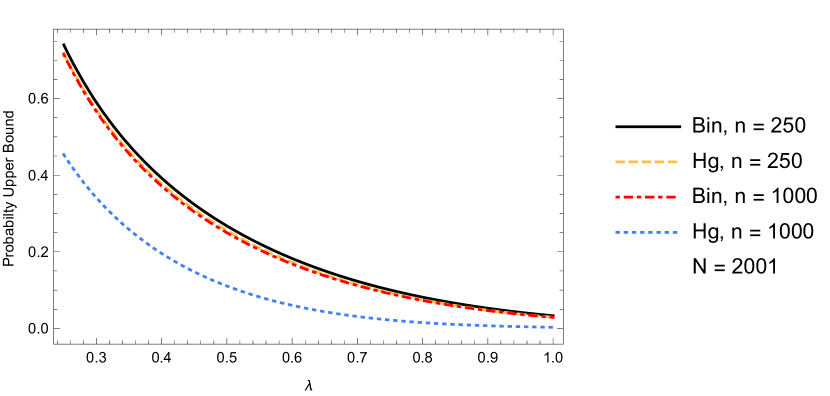
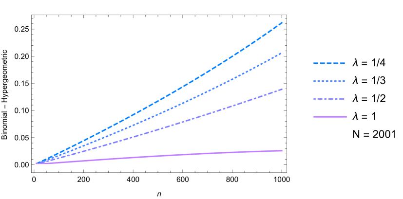
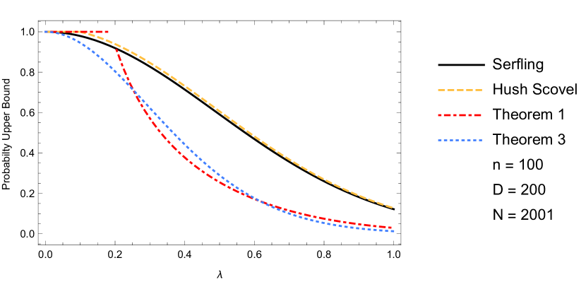
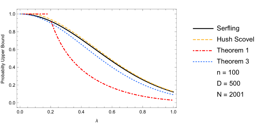
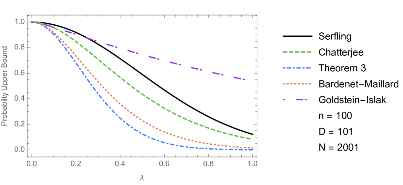
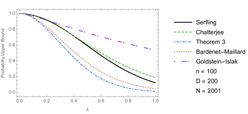
Figure 1 demonstrates the benefit of including a finite-sampling correction factor inside the exponential term: when enough of the the population is sampled, the difference between the binomial and hypergeometric bounds can differ by as much as $1/4$ for specific deviation values. Figure 2 compares the performance of the new hypergeometric bounds to each other and to the bounds of Serfling (1.1) and Hush and Scovel (1.5). It also provides some insight as to when (2.4) out-performs (2.7) and vice-versa. The finite-but-unspecified constants appearing in (2.5) prevent its inclusion in the figures. Additionally, the constants are not immediately comparable to those in (2.2) because they depend on how one chooses to truncate the sampling fraction and population proportion. The bound (2.5) demonstrates that the factor $1-n/N$ in the exponential may apply for all $\lambda>0$ as long as a suitable leading constant is selected.

Chatterjee [3] used Stein’s method to derive very general concentration bounds for statistics based on random permutations. For example, here is a restatement of his Proposition 1.1: let $\{a_{i,j}:1\leq i,j\leq N\}$ be a collection of numbers in $[0,1]$ and let $S\equiv\sum_{i=1}^{N}a_{i,\pi(i)}$ where $\pi\sim\$uniformly on all permutations of $\{1,\ldots,N\}$. Then

$$P(|S-E(S)|\geq t)\leq 2\exp\left(-\frac{t^{2}}{4E(S)+2t}\right)\ \ \ \mbox{for all}\ \ t>0.$$

The statistic $S$ was first studied by Hoeffding [9]. The special case which yields the setting of Serfling’s inequality is $a_{i,j}:=1_{[i\leq n]}c_{j}$ for $1\leq i,j\leq N$ where $1\leq n<N$. Then $S=\sum_{i=1}^{n}c_{\pi(i)}\stackrel{{\scriptstyle d}}{{=}}S_{n}$ where $S_{n}=\sum_{i=1}^{n}X_{i}$ is as defined in the first paragraph of section 1 above. In this special case $E(S)=n\overline{c}_{N}=n\mu$ and Chatterjee’s (Bernstein type) bound becomes

$$P(n^{-1/2}(S_{n}-n\mu)\geq\lambda)\leq\exp\left(-\frac{\lambda^{2}}{4\overline{c}_{N}+2\lambda/\sqrt{n}}\right)$$ (2.10)

for all $\lambda>0$.

Goldstein and Işlak [6] recently used a variant of Stein’s method to give another inequality for the tails of Hoeffding’s statistic $S$:

$$P(|S-E(S)|>t)\leq 2\exp\left(-\frac{t^{2}}{2(\sigma_{A}^{2}+8\|a\|t)}\right)$$ (2.11)

where $\|a\|\equiv\max_{i,j\leq N}|a_{i,j}-a_{i\cdot}|$,

$$a_{i\cdot} = \frac{1}{N}\sum_{j=1}^{N}a_{ij},\ \ \ a_{\cdot j}=\frac{1}{N}\sum_{i=1}^{N}a_{ij},\ \ \ a_{\cdot\cdot}=\frac{1}{N^{2}}\sum_{i,j=1}^{N}a_{ij},\ \ \mbox{and}$$

$$\sigma_{A}^{2} = \frac{1}{N-1}\sum_{i,j\leq N}(a_{ij}-a_{i\cdot}-a_{\cdot j}+a_{\cdot\cdot})^{2}.$$

Specializing (2.11) to the setting of Serfling’s inequality (with $a_{i,j}:=1_{[i\leq n]}c_{j}$) yields

$$P(n^{-1/2}|S_{n}-n\overline{c}_{N}|>\lambda)\leq 2\exp\left(-\frac{\lambda^{2}/2}{\sigma_{c}^{2}(1-f_{n})+8\|c\|\lambda/\sqrt{n}}\right)$$ (2.12)

where $\sigma_{c}^{2}=N^{-1}\sum_{j=1}^{N}(c_{j}-\overline{c}_{N})^{2}$ and $\|c\|\equiv\max_{j\leq N}|c_{j}-\overline{c}_{N}|$. This Bernstein type bound is in the same setting as Serfling’s inequality, but the bound has an explicit dependence on $\sigma_{c}^{2}$. This is similar to the bound of Bardenet and Maillard (1.6) which incorporates variance information through the parameter $\gamma^{2}$.

Further specialization of (2.12) to the (one-sided) hypergeometric setting (with $c_{j}=1\{j\leq D\}$ for $j=1,\ldots,N$) yields

$$P(n^{-1/2}(S_{n}-n(D/N))>\lambda)$$

$$\leq \exp\left(-\frac{\lambda^{2}/2}{(D/N)(1-D/N)(1-f_{n})+8\{(D/N)\vee(1-D/N)\}\lambda/\sqrt{n}}\right)$$

$$= \exp\left(-\frac{\lambda^{2}/2}{\sigma_{N}^{2}(1-f_{n})+8\{\mu_{N}\vee(1-\mu_{N})\}\lambda/\sqrt{n}}\right).$$

This bound differs from the bound given in (2.9) (the Bernstein type corollary of Theorem 3) only through the second term in the denominator inside the exponential: note that $8\{\mu_{N}\vee(1-\mu_{N})\}\geq 4>1/3$.

Comparing the Bernstein type bounds (2.12) and (2) to Serfling’s inequality (1.3) with $b=1$ and $a=0$, we see that the bound of Goldstein and Işlak is smaller than Serfling’s bound when $\lambda\leq\sqrt{n}/(32(\overline{c}_{N}\vee(1-\overline{c}_{N})))(1-4\sigma_{N}^{2}+4\sigma_{N}^{2}f_{n}-f_{n}^{*})$. Similarly, we see that Chatterjee’s bound (2.10) is smaller than Serfling’s bound only if $\overline{c}_{N}\leq(1-(n-1)/N)/8$ and then $\lambda\leq\sqrt{n}(1-(n-1)/N-8\overline{c}_{N})/4$. Figure 3 gives a comparison of Serfling’s bound, Chatterjee’s bound, Bardenet and Maillard’s bound (1.6), Goldstein and Işlak’s bound (2), and the Bennett type bound (2.7) in the further hypergeometric special case with $n=100$, $N=2001$, and $D\in\left\{101,200\right\}$; note that in the case $D=200$, $\overline{c}_{N}=D/N\approx.10$ so $8\overline{c}_{N}\approx.8$ while $1-(n-1)/N)\approx 1-.05$ so the first condition holds and then Chatterjee’s bound should win approximately when $\lambda\leq\sqrt{n}(.15)/4\approx 1.5/4$.

Comparing (2) to (2.10), we find the Goldstein-Işlak bound improves Chatterjee’s bound when $\lambda\leq\sqrt{n}(2\overline{c}_{N}-\sigma_{N}^{2}(1-f_{n}))/(8(\overline{c}_{N}\vee(1-\overline{c}_{N}))-1)$. In figure 3, this region is approximately equal to $\lambda\leq 0.08$ when $D=101$ and $\lambda\leq 0.18$ when $D=200$. From Figure 3(b) we see that the improvement of Goldstein and Işlak’s bound to those of Chatterjee and Serfling is very small in this region. From Figure 3(a) we see that Chatterjee’s bound is smaller than both the Goldstein and Işlak bound (2) as well as Serfling’s bound, when $D/N$ is small and $0.08\leq\lambda\leq\sqrt{n}(.55)/4\approx 1.37$, but that all three are improved by Bardenet and Maillard’s bound (1.6) and the Bennett type bound (2.7).

(a) 1a

(b) 1b

Figure 1: Comparison of León and Perron’s binomial bound (2.1) to the new hypergeometric bound (2.4). In sub-figure 1(a), the sample size $n$ is set to $250$ and $1000$ for both bounds. The population size $N$ is taken to be $2001$ in both cases. In the legend, lines with the description “Bin” correspond to the binomial bound of León and Perron (2.1), while lines with the description “Hg” correspond to the new hypergeometric bound (2.4). In sub-figure 1(b), we plot the difference between León and Perron’s binomial bound (2.1) to the new hypergeometric bound (2.4) at the fixed deviation-values $\lambda\in\left\{1/4,1/3,1/2,1\right\}$. We let $n$ vary between $10$ and $1000$ to illustrate the impact of introducing the finite-sampling correction factor into the exponential term of the probability bound.

(a) 2a

(b) 2b

Figure 2: These plots compare the various exponential bounds for the Hypergeometric distribution. In these plots we fix the population to $N=2001$, and the sample size to $n=100$. The plots consider a setting with smaller variances by setting $D=200$ in the first plot (so $D/N=1/10$) and $D=500$ in the second (so $D/N=1/4$). We see that the bound of Theorem 1 (2.4) performs comparably with the bound of Theorem 3 (2.7) in the setting $D=200$ (2a), and surpasses it when $D=500$ (2b). This suggests that when $D/N<1/10$, the bound of Theorem 3 will perform better than the bound of Theorem 1, and when $1/10\leq D/N<1/2$, the converse.

(a) 1a

(b) 1b

Figure 3: Comparison of Serfling’s bound (1.3), Chatterjee’s bound (2.10), and the bound of Goldstein and Işlak (2), Bardenet and Maillard’s bound (1.6), and Theorem 3. In sub-figure 3(a), the sample size is $n=100$, the population size is $N=2001$, and the number of successes is $D=101$. In sub-figure 3(b), the sample size remains $n=100$, the population size remains $N=2001$, but $D=200$.

3 Convex Order for the Hypergeometric Distribution

When sampling without replacement from a finite population concentrated on $[0,1]$, the hypergeometric distribution occupies an extreme position with respect to convex order. This extreme position offers additional reason to give the hypergeometric distribution special consideration, since we might hope to adapt bounds for its tail to the tails of the random variables it dominates through the convex order.

The extreme position of the hypergeometric distribution was essentially proved by Kemperman [14]. In his paper Kemperman studied (among many other things) finite populations majorized by nearly Rademacher populations; through transformation, this describes the hypergeometric setting. We say nearly Rademacher since Kemperman’s analysis resulted in majorizing populations consisting entirely of $-1^{\prime}s$ and $1^{\prime}s$ with the exception of a single exceptional element $\alpha$ with $-1<\alpha<1$.

Here, we revisit his argument, modified so it applies to a population with elements between $0$ and $1$. We then provide an extension of the argument in order to obtain a hypergeometric population which sub-majorizes this initial population. Since the extension follows naturally from Kemperman’s majorization result, we begin with his procedure here. We start with relevant definitions from Marshall, Olkin, and Arnold [16].

Definition 1.

For a vector $\mathbb{x}=(x_{1},\dots,x_{N})\in\mathbb{R}^{N}$, let

$$x_{[1]}\geq x_{[2]}\geq\dots\geq x_{[N]}$$

denote the components of $\mathbb{x}$ in decreasing order.

Definition 2.

For $\mathbb{x},\mathbb{y}\in\mathbb{R}^{N}$,

$$\mathbb{x}\prec\mathbb{y}\ \text{ if }\ \begin{cases}\sum_{i=1}^{k}x_{[i]}\leq\sum_{i=1}^{k}y_{[i]},\ k=1,\dots,N-1,\\ \sum_{i=1}^{N}x_{[i]}=\sum_{i=1}^{N}y_{[i]}\\ \end{cases}$$

where $\mathbb{x}\prec\mathbb{y}$ is read as “$\mathbb{x}$ is majorized by $\mathbb{y}$”.

Definition 3.

For $\mathbb{x},\mathbb{y}\in\mathbb{R}^{N}$,

$$\mathbb{x}\prec_{w}\mathbb{y}\ \text{ if }\ \sum_{i=1}^{k}x_{[i]}\leq\sum_{i=1}^{k}y_{[i]},\ k=1,\dots,N$$

where $\mathbb{x}\prec_{w}\mathbb{y}$ is read as “$\mathbb{x}$ is weakly sub-majorized by $\mathbb{y}$” or, more briefly, “$\mathbb{x}$ is sub-majorized by $\mathbb{y}$”.

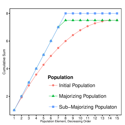
Figure 4 provides an illustration of these definitions. In the following Lemma, we re-state Kemperman’s procedure so it constructs a majorizing hypergeometric population. See section 4, pages 165–168 in [14] for the original Rademacher argument.

Figure 4: The initial population line in the display coresponds to $\mathbb{c}=\left\{0,1/14,2/14,\dots,13/14,1\right\}$. The majorizing population contains seven $0^{\prime}s$, seven $1^{\prime}s$, and a single exceptional element of $1/2$. The sub-majorizing population contains seven $0^{\prime}s$ and eight $1^{\prime}s$. In the display, each population is sorted in decreasing order; the corresponding lines show the cumulative sum of the ordered population elements.

Lemma 1.

(Kemperman [14]) For any finite population $\mathbb{x}\in\mathbb{R}^{N}$, such that $0\leq x_{i}\leq 1$ for all $1\leq i\leq N$, there exists a population $\mathbb{c}\in\mathbb{R}^{N}$, consisting only of $0$’s, $1$’s, and at most a single element between $0$ and $1$, which majorizes the original population. In fact, $\mathbb{c}$ consists of $D$ $1$’s, $N-D-1$ $0$’s, and a number $\alpha\in[0,1)$ where $D$ and $\alpha$ are determined by $D=\lfloor N\bar{\mathbb{x}}_{N}\rfloor$, and $\alpha=N\bar{\mathbb{x}}_{N}-D$.

Algorithm 1 Kemperman’s majorization algorithm

1:function Majorize($ipop$)$\triangleright$ $ipop$ is the input population

2:     $plen\leftarrow\text{length}(ipop)$

3:     $mpop\leftarrow ipop$ $\triangleright$ Make a copy of the input population to transform

4:     for $i\in\left\{1,\dots,plen-1\right\}$ do

5:         $csum\leftarrow mpop[i]+mpop[i+1]$

6:         if $csum>1$ then

7:              $mpop[i]\leftarrow 1$

8:              $mpop[i+1]\leftarrow(csum-1)$

9:         else

10:              $mpop[i]\leftarrow 0$

11:              $mpop[i+1]\leftarrow csum$               

12:     return $mpop$$\triangleright$ mpop is now transformed into the desired population

Proof.

We update Kemperman’s argument, and demonstrate his modified algorithm described in the display produces the population claimed by Lemma 1. Suppose first that $\mathbb{x}\in\mathbb{R}^{2}$, and $0\leq x_{1},x_{2}\leq 1$. Identify $ipop=\mathbb{x}$ in the algorithm description. Then $mpop=\mathbb{x}$, $plen=2$, and $plen-1=1$. Hence, the “for” loop executes exactly once.

Consider the operations in the “for” loop. We compute $csum=mpop[1]+mpop[2]=x_{1}+x_{2}$. If $csum>1$, the first condition is met, and we set $mpop[1]=1$ and $mpop[2]=csum-1$. Since $csum=x_{1}+x_{2}$, and $0\leq x_{1},x_{2}\leq 1$ by assumption, we have $1<csum\leq 2$. Hence $0<csum-1\leq 1$, and so $0<mpop[2]\leq 1$. Observe, that $mpop[1]=1\geq x_{1}\vee x_{2},$ $mpop[1]+mpop[2]=1+(x_{1}+x_{2}-1)=x_{1}+x_{2}$, so that mpop now majorizes $\mathbb{x}$ as claimed. If $csum\leq 1$, the algorithm sets $mpop[2]=x_{1}+x_{2}$, and $mpop[1]=0$. Again, this satisfies the description in the lemma, since $0\leq csum=x_{1}+x_{2}\leq 1$. Moreover, $mpop[2]=x_{1}+x_{2}\geq x_{1}\vee x_{2}$ and $mpop[2]+mpop[1]=x_{1}+x_{2}+0=x_{1}+x_{2}$, and so again $mpop$ majorizes the population $\mathbb{x}$. This completes the base case. Observe that the exceptional element is in the final index of the vector.

For the inductive case, suppose Kemperman’s algorithm works when $n=N$. We will show it holds for $n=N+1$. Let $\mathbb{x}\in\mathbb{R}^{N+1}$ be a population whose elements are all between $0$ and $1$. Let $\mathbb{y}\in\mathbb{R}^{N}$ be constructed so that $y_{i}=x_{i}$ for $1\leq i\leq N$. Run the algorithm on $\mathbb{y}$. By the induction hypothesis, this produces a vector $\mathbb{m}\in\mathbb{R}^{N}$, such that $m_{i}\in\left\{0,1\right\}$ for $1\leq i\leq N-1$. Moreover, $0\leq m_{N}\leq 1$ by the induction hypothesis, and also $\mathbb{m}$ majorizes $\mathbb{y}$.

Next, construct a vector $\mathbb{a}\in\mathbb{R}^{2}$ such that $a_{1}=m_{N}$ and $a_{2}=x_{N+1}$. Run the algorithm on $\mathbb{a}$. By the base case, this produces a new vector $\mathbb{b}\in\mathbb{R}^{2}$ such that $b_{1}\in\left\{0,1\right\}$ and $0\leq b_{2}\leq 1$. Note also that $\mathbb{b}$ majorizes $\mathbb{a}$.

Finally, construct a vector $\mathbb{c}\in\mathbb{R}^{N+1}$ such that $c_{i}=m_{i}$ for $1\leq i\leq N-1$, $c_{N}=b_{1}$ and $c_{N+1}=b_{2}$. By construction, we have that $c_{i}\in\left\{0,1\right\}$ for $1\leq i\leq N$ and $0\leq c_{N+1}\leq 1$. Hence, if we can show that $\mathbb{c}$ majorizes $\mathbb{x}$ we are done. We first show that

$$\sum_{i=1}^{N+1}c_{i}=\sum_{i=1}^{N+1}x_{i}\ .$$

Using the constructions, we have

$$\sum_{i=1}^{N+1}c_{i} =\left[\sum_{i=1}^{N-1}c_{i}\right]+c_{N}+c_{N+1}=\left[\sum_{i=1}^{N-1}m_{i}\right]+b_{1}+b_{2}=\left[\sum_{i=1}^{N-1}m_{i}\right]+m_{N}+x_{N+1}$$

$$=\left[\sum_{i=1}^{N}m_{i}\right]+x_{N+1}=\left[\sum_{i=1}^{N}y_{i}\right]+x_{N+1}=\left[\sum_{i=1}^{N}x_{i}\right]+x_{N+1}=\sum_{i=1}^{N+1}x_{i}\ ,$$

and so the summation claim holds. Next, pick $1\leq k\leq N+1$. Then

$$\sum_{i=1}^{k}c_{[i]}\geq\sum_{i=1}^{k}x_{[i]}$$

since by construction, $c_{i}\in\left\{0,1\right\}$ for $1\leq i\leq N$. As $0\leq x_{i}\leq 1$ for $1\leq i\leq N+1$, if $k$ is small enough so that

$$\sum_{i=1}^{k}c_{[i]}<\sum_{i=1}^{N+1}c_{[i]}=\sum_{i=1}^{N+1}c_{i}\ ,$$

then all terms in the summation

$$\sum_{i=1}^{k}c_{[i]}$$

must be $1$, and so are greater than or equal to the corresponding $x$’s. If $k$ is large enough so that

$$\sum_{i=1}^{k}c_{[i]}=\sum_{i=1}^{N+1}c_{i}$$

(which means the remaining $N+1-k$ elements are all $0$), then we also have

$$\sum_{i=1}^{k}c_{[i]}\geq\sum_{i=1}^{k}x_{[i]}$$

since we have already seen that the sum over all the $x$’s equals the sum over all the $c$’s. As all the $x$’s are between $0$ and $1$ by assumption, this proves the claim. ∎

Lemma 2.

For any finite population $\mathbb{x}\in\mathbb{R}^{N}$, such that $0\leq x_{i}\leq 1$ for all $1\leq i\leq N$, there exists a population $\mathbb{z}\in\mathbb{R}^{N}$, consisting only of $0$’s and $1$’s, which sub-majorizes the original population.

Proof.

Consider a finite population $\mathbb{x}\in\mathbb{R}^{N}$ which obeys the hypotheses. Using Lemma 1, we may construct a population $\mathbb{y}\in\mathbb{R}^{N}$ which majorizes $\mathbb{x}$. By Lemma 1, we know that $\mathbb{y}$ consists only of $0$’s, $1$’s, and at most a single exceptional element $y_{N}$ between $0$ and $1$.

If the exceptional element is either exactly $0$ or exactly $1$, we are done. So, suppose $0<y_{N}<1$. Create a new population $\mathbb{z}\in\mathbb{R}^{N}$ such that $z_{i}=y_{i}$ for $1\leq i\leq N-1$, and $z_{N}=1$. This population $\mathbb{z}$ then sub-majorizes $\mathbb{y}$ and hence sub-majorizes $\mathbb{x}$, completing the proof.∎

Lemma 3.

Suppose $\mathbb{x}\in\mathbb{R}^{N}$ is a population consisting only of $0$’s, $1$’s, and a single exceptional element, $x_{1}$, such that $0<x_{1}<1$. Suppose $\mathbb{y}\in\mathbb{R}^{N}$ is a population whose elements are the same as those in $\mathbb{x}$, except $y_{1}=1$ and so $y_{1}>x_{1}$. Let $X_{1},\dots,X_{n}$ denote a sample without replacement from $\mathbb{x}$, and $Y_{1},\dots,Y_{n}$ denote a sample without replacement from $\mathbb{y}$, $1\leq n\leq N$. Finally, suppose $\phi$ is a continuous convex increasing function on $\mathbb{R}$. Then

$$E\phi\left(\sum_{i=1}^{n}X_{i}\right)\leq E\phi\left(\sum_{i=1}^{n}Y_{i}\right)\ .$$ (3.1)

Proof.

We adapt Kemperman’s (1973) argument for Rademacher populations to the current setting of hypergeometric sub-majorization.

Observe that

$$E\phi\left(\sum_{i=1}^{n}X_{i}\right)=\frac{1}{{N\choose n}}\sum\phi\left(x_{i_{1}}+\dots+x_{i_{n}}\right)$$

where the sum is over all sets of indices $1\leq i_{1}<i_{2}<\dots<i_{n}\leq N$. Note the same holds for sampling without replacement from $\mathbb{y}$, with suitable substitution. Therefore

$${{N\choose n}}\left[E\phi\left(\sum_{i=1}^{n}Y_{i}\right)-E\phi\left(\sum_{i=1}^{n}X_{i}\right)\right] =\sum\begin{pmatrix}\phi\left(y_{1}+y_{i_{2}}+\dots+x_{i_{n}}\right)-\phi\left(x_{1}+x_{i_{2}}+\dots+x_{i_{n}}\right)\\ \end{pmatrix}$$

where the sum is over all distinct indices $2\leq i_{2}<i_{3}<\dots<i_{n}\leq N$. Note that sets of indices with $i_{1}>1$ cancel out by definition of the two populations. Since $\phi$ is assumed convex increasing, each term of the sum is non-negative. Hence, the entire sum is non-negative as well. This gives the claim. ∎

We next specialize a proposition stated in Marshall, Olkin, and Arnold [16, p. 455] to the current problem. Proof of the general statement given in the text is credited to Karlin; proof for the specific cases of sampling with and without replacement to Kemperman. As proof is given in Marshall, Olkin, and Arnold, we simply state the result here.

Lemma 4.

Let $\mathbb{x}\in\mathbb{R}^{N}$ be an arbitrary finite population. Let $\mathbb{y}\in\mathbb{R}^{N}$ be a finite population which majorizes $\mathbb{x}$. Let $X_{1},\dots,X_{n}$ denote a sample without replacement from $\mathbb{x}$, and $Y_{1},\dots,Y_{n}$ denote a sample without replacement from $\mathbb{y}$, $1\leq n\leq N$. Finally, suppose $\phi$ is a continuous convex increasing function on $\mathbb{R}$. Then

$$E\phi\left(\sum_{i=1}^{n}X_{i}\right)\leq E\phi\left(\sum_{i=1}^{n}Y_{i}\right)\ .$$

Note that Lemma 4 requires majorization between populations. We may combine the preceding lemmas to demonstrate the following claim.

Theorem 4.

For any finite population $\mathbb{x}\in\mathbb{R}^{N}$, such that $0\leq x_{i}\leq 1$ for all $1\leq i\leq N$, there exists a population $\mathbb{y}\in\mathbb{R}^{N}$, consisting only of $0$’s and $1$’s which sub-majorizes the original population. Let $X_{1},\dots,X_{n}$ denote a sample without replacement from $\mathbb{x}$, and $Y_{1},\dots,Y_{n}$ denote a sample without replacement from $\mathbb{y}$, $1\leq n\leq N$. Finally, suppose $\phi$ is a continuous convex increasing function on $\mathbb{R}$. Then

$$E\phi\left(\sum_{i=1}^{n}X_{i}\right)\leq E\phi\left(\sum_{i=1}^{n}Y_{i}\right)\ .$$

Proof.

Suppose $\mathbb{x}\in\mathbb{R}^{N}$ is a finite population which satisfies the hypotheses. We may use Lemma 1 to construct a population $\mathbb{z}\in\mathbb{R}^{N}$ such that $\mathbb{z}$ majorizes $\mathbb{x}$, and $\mathbb{z}$ consists only of $0$’s, $1$’s, and at most a single exceptional element between $0$ and $1$. For $1\leq n\leq N$, let $Z_{1},\dots,Z_{n}$ denote a sample without replacement from $\mathbb{z}$. By Lemma 4, we then have the order

$$E\phi\left(\sum_{i=1}^{n}X_{i}\right)\leq E\phi\left(\sum_{i=1}^{n}Z_{i}\right)\ .$$ (3.2)

Next, by Lemma 2 we may construct a population $\mathbb{y}\in\mathbb{R}^{N}$ consisting only of $0$’s and $1$’s that sub-majorizes $\mathbb{z}$. Then by (3.1) we have

$$E\phi\left(\sum_{i=1}^{n}Z_{i}\right)\leq E\phi\left(\sum_{i=1}^{n}Y_{i}\right)\ .$$ (3.3)

Combining (3.2) and (3.3) proves the claim. ∎

Inequality (2.7) provides an opportunity to apply Theorem 4. Recalling the notation of the introduction, let $\mathbb{c}:=\left\{c_{1},\dots,c_{N}\right\}$ be a population such that $0\leq c_{i}\leq 1$ for $1\leq i\leq N$, $a=0$, $b=1$, and $\overline{c}_{N}+1/N\leq 1/2$. Using Kemperman’s algorithm, as stated in Lemma 1, there exists a population $\mathbb{m}:=\left\{m_{1},\dots,m_{N}\right\}$ which majorizes $\mathbb{c}$ such that $m_{i}\in\left\{0,1\right\}$ for $1\leq i\leq N-1$, and $0\leq m_{N}\leq 1$. In the following, suppose $0<m_{N}<1$, since if $m_{N}=0$ or $m_{N}=1$ we can apply (2.7) directly.

Since $\mathbb{c}\prec\mathbb{m}$, we have $\overline{m}_{N}=\overline{c}_{N}$. Using Lemma 2, there is a population $\left\{h_{1},\dots,h_{N}\right\}$ with $h_{i}\in\left\{0,1\right\}$ for $1\leq i\leq N$ that sub-majorizes $\mathbb{c}$. By the preceding construction, we have $h_{i}=m_{i}$ for $1\leq i\leq N-1$, and $h_{N}\equiv 1>m_{N}$.

Without loss of generality, re-label $\mathbb{m}$ and $\mathbb{h}$ so that: for $1\leq i\leq D-1$ we have $h_{i}=m_{i}=1$; for $i=D$ we have $h_{D}=1>m_{D}>0$; for $D+1\leq i\leq N$ we have $h_{i}=m_{i}=0$. Denote the exceptional element of $\mathbb{m}$ by $\alpha:=m_{D}$. With the populations so modified, we derive bounds for the difference between the populations means:

$$\frac{1}{N}\geq\overline{h}_{N}-\overline{m}_{N}=\frac{h_{D}-m_{D}}{N}=\frac{1-\alpha}{N}\geq 0\ .$$ (3.4)

By construction, we thus have

$$\overline{m}_{N}\leq\overline{h}_{N}\leq\overline{m}_{N}+\frac{1}{N}\leq\frac{1}{2}\ .$$

Suppose then that we sample $n<D$ items without replacement from $\mathbb{c}$. Let $X_{i}$ denote the sample without replacement from $\mathbb{c}$, and let $H_{i}$ denote a corresponding sample without replacement from $\mathbb{h}$. Then for $t>0$

$$P\left(\sum_{i=1}^{n}X_{i}-n\mu_{c}\geq t\right)\leq\ \inf_{r>0}\frac{E\exp\left(r\sum_{i=1}^{n}X_{i}\right)}{\exp\left(rt+rn\mu_{c}\right)}$$

$$\leq\ \inf_{r>0}\frac{E\exp\left(r\sum_{i=1}^{n}H_{i}\right)}{\exp\left(rt+rn\mu_{c}\right)}$$ (3.5)

$$=\ \inf_{r>0}\exp\left(rn(\mu_{h}-\mu_{c})\right)\frac{E\exp\left(r\sum_{i=1}^{n}(H_{i}-\mu_{h})\right)}{\exp\left(rt\right)}$$

$$\leq\ \inf_{r>0}\exp\left(r\frac{n}{N}\right)\frac{E\exp\left(r\sum_{i=1}^{n}(H_{i}-\mu_{h})\right)}{\exp\left(rt\right)}$$ (3.6)

$$=\ \inf_{r>0}\exp\left(r\frac{n}{N}\right)\frac{E\exp\left(r\sum_{i=1}^{n}(Y_{i}-\pi_{i})\right)}{\exp\left(rt\right)}$$

$$\leq\ \inf_{r>0}\exp\left(r\frac{n}{N}-rt+n\left(\frac{\sum_{i=1}^{n}\pi_{i}(1-\pi_{i})}{n}\right)\left(e^{r}-1-r\right)\right)$$ (3.7)

$$=\ \inf_{r>0}\exp\left(r\frac{n}{N}-rt+n\gamma^{2}\left(e^{r}-1-r\right)\right)$$ (3.8)

where in the final line we write $\gamma^{2}:=(1/n)\sum_{i=1}^{n}\pi_{i}(1-\pi_{i})$. The inequality at (3.6) follows by (3.4). The inequality at (3.5) follows by Theorem 4. The inequality at line (3.7) follows by Shorack and Wellner page 852, display (b) [20].

At this point we may continue from (3.8) and optimize over $r$. Doing so yields an optimal choice of

$$r^{*}=\log\left(1+\frac{Nt-n}{nN\gamma^{2}}\right)\ .$$

Using this value, however, yields an exponential bound that is somewhat difficult to compare to (2.7). If instead we simply choose

$$r^{*}_{2}=\log\left(1+\frac{t}{n\gamma^{2}}\right)\ ,$$

we obtain a bound similar in performance to the bound we find using $r^{*}$, but has the benefit of easy comparison to (2.7). The choice $r_{2}^{*}$ corresponds to the optimal value of $r$ when the original population is majorized by a hypergeometric population. We continue from (3.8) using $r_{2}^{*}$, and obtain

$$P\left(\sum_{i=1}^{n}X_{i}-n\mu_{c}\geq t\right)\leq \exp\left(\frac{n}{N}\log\left(1+\frac{t}{n\gamma^{2}}\right)\right)\cdot\exp\left(-t\left[\left(1+\frac{n\gamma^{2}}{t}\right)\log\left(1+\frac{t}{n\gamma^{2}}\right)-1\right]\right)$$

$$= \exp\left(\frac{n}{N}\log\left(1+\frac{t}{n\gamma^{2}}\right)\right)\cdot\exp\left(-\frac{t^{2}}{2n\gamma^{2}}\psi\left(\frac{t}{n\gamma^{2}}\right)\right)\ .$$ (3.9)

Writing $\lambda=t/\sqrt{n}$ , and substituting $\gamma^{2}=(D/N)(1-D/N)(1-f_{n})\equiv\sigma_{N}^{2}(1-f_{n})$, we obtain the following bound:

$$P(\sqrt{n}(\overline{X}_{n}-\mu_{c})\geq\lambda)\leq\left(1+\frac{\lambda}{\sqrt{n}\sigma_{N}(1-f_{n})}\right)^{n/N}\exp\left(-\frac{\lambda^{2}}{2\sigma_{N}^{2}(1-f_{n})}\psi\left(\frac{\lambda}{\sqrt{n}\sigma_{N}^{2}(1-f_{n})}\right)\right)\ .$$

In this form, the cost of sub-majorization is clear when compared to (2.7): we incur the leading term outside the exponent. By shifting and scaling the population, we may use this bound to obtain the following theorem for the general problem of sampling without replacement:

Theorem 5.

Let $\mathbb{c}:=\left\{c_{1},\dots,c_{N}\right\}$ be a population with $a=\min_{1\leq i\leq N}c_{i}$ and $b=\max_{1\leq i\leq N}c_{i}$ both finite. Let $\mathbb{d}:=\left\{(c_{1}-a)/(b-a),\dots,(c_{N}-a)/(b-a)\right\}$. Suppose first that $\mathbb{d}$ is majorized by a Hypergeometric population such that $D/N\leq 1/2$. From this Hypergeometric population define $\sigma_{N}^{2}:=(D/N)(1-D/N)$. Then the following bound holds for a sample without replacement of $n<D$ items from $\mathbb{c}$:

$$P(\sqrt{n}(\overline{X}_{n}-\mu_{c})\geq\lambda)\leq\exp\left(-\frac{\lambda^{2}}{2(b-a)^{2}\sigma_{N}^{2}(1-f_{n})}\psi\left(\frac{\lambda}{\sqrt{n}(b-a)\sigma_{N}^{2}(1-f_{n})}\right)\right)\ .$$ (3.10)

If instead $\overline{d}_{N}+1/N\leq 1/2$, then the following bound holds for a sample without replacement of $n<D$ items from $\mathbb{c}$:

$$P(\sqrt{n}(\overline{X}_{n}-\mu_{c})\geq\lambda)$$

$$\leq\ \ \left(1+\frac{\lambda}{\sqrt{n}(b-a)\sigma_{N}(1-f_{n})}\right)^{n/N}\cdot\exp\left(-\frac{\lambda^{2}}{2(b-a)^{2}\sigma_{N}^{2}(1-f_{n})}\psi\left(\frac{\lambda}{\sqrt{n}(b-a)\sigma_{N}^{2}(1-f_{n})}\right)\right)\ .$$ (3.11)

Two-sample rank tests provide an opportunity to explore the behavior of the bounds of Theorem 5. Following the exposition in Chapter 4 of Hájek, Šidák, and Sen [8] (with the notation modified), let $Y_{1},\dots,Y_{n}$ and $Z_{1},\dots,Z_{m}$ be random samples with continuous distributions $F_{Y}$ and $F_{Z}$. Form the pooled sample $Y_{n+j}=Z_{j}$, $j=1,\dots,m$, and $N=n+m$. Let $R_{i}\ (i=1,\dots,N)$ denote the rank of the observation $Y_{i}$ in the ordered sequence $Y_{(1)}<Y_{(2)}<\dots<Y_{(N)}$. To test the null hypothesis $H_{0}:F_{Y}=F_{Z}$ against alternatives of shifts in location, one may use the Wilcoxon test (see page 96 [8]). The test statistic, expectation under the null, and variance under the null are

$$S_{W}:=\sum_{i=1}^{n}R_{i}\ ,ES_{W}=\frac{1}{2}n(n+m+1)\ ,\text{ and }Var(S_{W})=\frac{1}{12}nm(n+m+1)\ .$$

Under the null, $S_{W}$ may be viewed as the sum in a sample without replacement from the population $\mathbb{c}_{W}:=\left\{1,2,\dots,N\right\}$, where $a=1$ and $b=N$. Shifting and scaling the population produces $\mathbb{d}_{W}:=\left\{0,1/(N-1),\dots,(N-2)/(N-1),1\right\}$ . If $N$ is even, then $\mathbb{d}_{W}$ is majorized by a Hypergeometric population containing $N/2\ 1^{\prime}s$ and $N/2\ 0^{\prime}s$, and hence $\sigma^{2}_{N}=(D/N)(1-D/N)=1/4$. If we additionally assume $n\leq m$, we may use (3.10) to study its finite sample behavior. Doing so we find for $\lambda>0$

$$P\left(\sqrt{n}\left(\overline{X}_{n}-\frac{(N+1)}{2}\right)\geq\lambda\right)\leq\exp\left(-\frac{2\lambda^{2}}{(n+m-1)^{2}(1-f_{n})}\psi\left(\frac{2\lambda}{\sqrt{n}(n+m-1)(1-f_{n})}\right)\right)\ .$$

Serfling’s bound (1.1) may be applied in this case as well; through its application we find

$$P\left(\sqrt{n}\left(\overline{X}_{n}-\frac{(N+1)}{2}\right)\geq\lambda\right)\leq\exp\left(-\frac{2\lambda^{2}}{(n+m-1)^{2}(1-\frac{n-1}{n+m})}\right)\ .$$

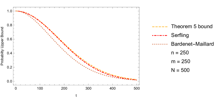
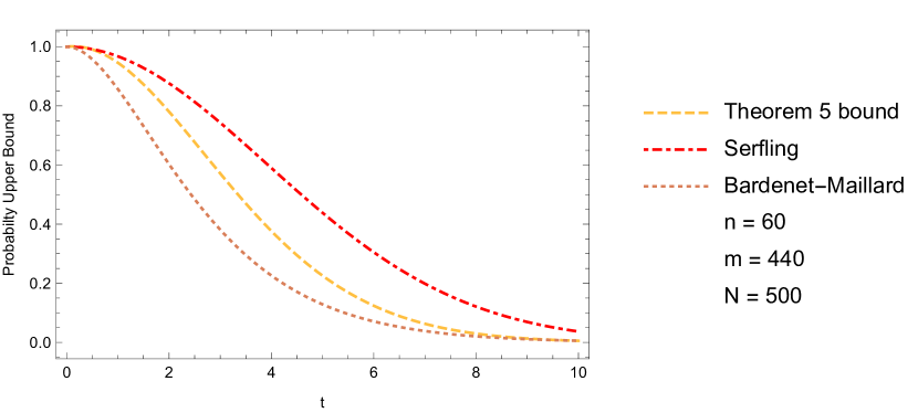
Finally, we may use Bardenet and Maillard’s bound (1.6) with $\delta=\delta_{f}=1\times 10^{-7}$ to analyze the situation as well. Figure 5 compares the performance of these three bounds when $n=m=250$. In this case, we see that the bounds are comparable, with Bardenet and Maillard’s bound performing the best, and Serfling’s performance superior to (3.10). This occurs because the variance component $(D/N)(1-D/N)$ (which is close to $1/4$ when $n=m=250$) that appears in the bound is the variance of the majorizing hypergeometric population rather than the variance of the shifted and scaled population $\mathbb{d}_{w}$ (which is close to $1/12$ when $n=m=250$). Bardenet and Maillard’s bound performs well because it incorporates information about the variance of the untransformed population into its bound.

Another example is found in the Klotz test, which is used to test the null $H_{0}:F_{Y}=F_{Z}$ against alternatives of differences in scale (see page 104 [8]). Recalling $N:=n+m$, the test statistic, expectation under the null, and variance under the null are

$$S_{K}:=\sum_{i=1}^{n}\left[\Phi^{-1}\left(\frac{R_{i}}{N+1}\right)\right]^{2}\ ,\ ES_{K}=\frac{n}{N}\sum_{i=1}^{N}\left[\Phi^{-1}\left(\frac{i}{N+1}\right)\right]^{2}\ ,$$

and

$$VarS_{K}=\frac{nm}{N(N-1)}\sum_{i=1}^{N}\left[\Phi^{-1}\left(\frac{i}{N+1}\right)\right]^{4}-\frac{m}{n(N-1)}(ES_{K})^{2}\ .$$

Defining the population

$$\mathbb{c}_{K}:=\left\{c_{i}:=\left[\Phi^{-1}\left(\frac{i}{N+1}\right)\right]^{2}\ ,\ 1\leq i\leq N\right\}\ ,$$

we may view $S_{K}$ under the null as the sum in a sample without replacement from $\mathbb{c}_{K}$. If $n+m=500$, we may compute $\mathbb{c}_{K}$, and find $a\approx 6.26\times 10^{-6}$ and $b\approx 8.29$. Shifting and scaling the population produces $\mathbb{d}_{K}$, which is bounded by $0$ and $1$. This population is majorized by a population containing $59$ $1^{\prime}s$, $440$ $0^{\prime}s$, and a single exceptional element approximately equal to $0.044$. Hence, it is sub-majorized by a population containing $60$ $1^{\prime}s$ and $440$ $0^{\prime}s$. Supposing that $n=60$ and $m=440$, we may use (3.11) to analyze this scenario since the mean of the sub-majorizing population is $3/25$ (also note $(D/N)(1-D/N)=66/625$ in this case). Doing so (with the conservative approximation that $b-a\approx 8.29$), we find for $\lambda\geq 0$ that

$$P(\sqrt{60}(\overline{X}_{60}-\mu_{K})\geq\lambda)$$

$$\leq\ \ \left(1+\frac{\lambda}{\sqrt{60}(8.29)(66/625)(440/499)}\right)^{3/25}\cdot\exp\left(-\frac{\lambda^{2}}{2(8.29)^{2}(66/625)(440/499)}\psi\left(\frac{\lambda}{\sqrt{60}(8.29)(66/625)(440/499)}\right)\right)\ .$$

Once again, we may apply Serfling’s uniform bound. Doing so here, we find

$$P\left(\sqrt{60}(\bar{X}_{60}-\mu_{K})\geq\lambda\right)\leq\exp\left(-\frac{2\lambda^{2}}{(441/500)(8.29)^{2}}\right)\ .$$

As in the Wilcoxon example, we may use Bardenet and Maillard’s bound (1.6) with $\delta=\delta_{f}=1\times 10^{-7}$ to analyze the situation. Figure 5 also compares the performance of these three bounds for the special case $n=60$ and $m=440$. In this case, we again see that Bardenet and Maillard’s bound performs the best, but that the bound obtained via sub-majorization now improves on Serfling’s result. This is because the variance component of the sub-majorizing hypergeometric population, $(D/N)(1-D/N)=66/625=0.1056<1/4$ reflects some of the variability of the untransformed population. However, the untransformed population $d_{K}$ has variance $\sigma^{2}\approx 0.0258$; this variability is captured in the bound of Bardenet and Maillard, and so we see the improved performance.

Thus we see that (sub-)majorization, as a strategy for finding exponential bounds which incorporate information about the population variance in the problem of sampling without replacement from a bounded finite population, can produce sub-optimal results. As we saw, this is because the (sub-)majorizing hypergeometric population can be more variable than the underlying population from which we sample. However, if our goal is to find uniform exponential bounds, this information loss is immaterial: such bounds apply to all underlying populations, regardless of their variability. Hence the analysis of the hypergeometric distribution which produced Theorems 1 and 2. We turn to the proofs of these bounds in the concluding section.

(a) 1a

(b) 1b

Figure 5: Comparison of the bounds of Theorem 5 to Bardenet and Maillard’s bound (1.6) and Serfling’s bound. The first sub-figure (5(a)), corresponds to the Wilcoxon example. The second sub-figure (5(b)), corresponds to the Klotz example.

4 Proofs of the Bounds

Our proofs depend on a version of Stirling’s formula from Robbins [18].

Lemma 5.

For $n\in\mathbb{N}_{0}$

$$\sqrt{2\pi n}\left(\frac{n}{e}\right)^{n}e^{\frac{1}{12n+1}}\leq n!\leq\sqrt{2\pi n}\left(\frac{n}{e}\right)^{n}e^{\frac{1}{12n}}\ .$$ (4.1)

To prove (2.4), we will need some additional tools. We start with the following lemma.

Lemma 6.

Suppose $S_{n}\sim\text{Hypergeometric}(n,D,N)$ with $1\leq n<D\leq\lfloor N/2\rfloor$ and $1\leq k\leq n-1$. Then for $k\geq n(D/N)$ we have

$$P(S_{n}=k) \leq\frac{1}{\sqrt{2\pi}}\frac{\sqrt{D(N-D)n(N-n)}}{\sqrt{k(D-k)(n-k)(N-D-(n-k))N}}$$

$$\ \ \ \cdot\exp\left(-\frac{2nN}{N-n}u^{2}\right)\exp\left(-\frac{n}{3}\left(1+\frac{n^{3}}{(N-n)^{3}}\right)u^{4}\right)\ .$$ (4.2)

Proof.

The proof follows by direct analysis. Using Stirling’s formula (4.1), we have

$$P(S_{n}=k) =\frac{{D\choose k}{N-D\choose n-k}}{{N\choose n}}$$

$$\leq\frac{1}{\sqrt{2\pi}}\frac{\sqrt{D(N-D)n(N-n)}}{\sqrt{k(D-k)(n-k)(N-D-(n-k))N}}$$

$$\ \ \ \cdot\frac{D^{D}(N-D)^{N-D}n^{n}(N-n)^{N-n}}{k^{k}(D-k)^{D-k}(n-k)^{n-k}(N-D-(n-k))^{N-D-(n-k)}N^{N}}$$

$$\ \ \ \cdot\frac{\exp\left(\frac{1}{12D}+\frac{1}{12(N-D)}+\frac{1}{12n}+\frac{1}{12(N-n)}\right)}{\exp\left(\frac{1}{12k+1}+\frac{1}{12(D-k)+1}+\frac{1}{12(n-k)+1}+\frac{1}{12(N-D-(n-k))+1}+\frac{1}{12N+1}\right)}$$

$$=:A\cdot B\cdot C\ .$$ (4.3)

We consider the $B$ term first. Define $u:=k/n-\mu$, recalling $\mu:=D/N$. We then have

$$B =\frac{D^{D}(N-D)^{N-D}/N^{N}}{\left(\frac{k}{n}\right)^{k}\cdot\left(1-\frac{k}{n}\right)^{n-k}\cdot\left(\frac{D-k}{N-n}\right)^{D-k}\left(1-\frac{D-k}{N-n}\right)^{N-n-(D-k)}}$$

$$=\frac{\left(\frac{D}{N}\right)^{D}\left(1-\frac{D}{N}\right)^{N-D}}{\left(\frac{k}{n}\right)^{k}\left(1-\frac{k}{n}\right)^{n-k}\left(\frac{D-k}{N-n}\right)^{D-k}\left(1-\frac{D-k}{N-n}\right)^{N-n-(D-k)}}$$

$$=\frac{\left(\frac{D}{N}\right)^{D}}{\left(\frac{k}{n}\right)^{k}\left(\frac{D-k}{N-n}\right)^{D-k}}\cdot\frac{\left(1-\frac{D}{N}\right)^{N-D}}{\left(1-\frac{k}{n}\right)^{n-k}\left(1-\frac{D-k}{N-n}\right)^{N-n-(D-k)}}$$

$$=\frac{\left(\frac{D}{N}\right)^{k}\left(\frac{D}{N}\right)^{D-k}}{\left(\frac{k}{n}\right)^{k}\left(\frac{D-k}{N-n}\right)^{D-k}}\cdot\frac{\left(1-\frac{D}{N}\right)^{n-k}\left(1-\frac{D}{N}\right)^{N-D-(n-k)}}{\left(1-\frac{k}{n}\right)^{n-k}\left(1-\frac{D-k}{N-n}\right)^{N-n-(D-k)}}$$

$$=\left(\frac{\mu}{u+\mu}\right)^{k}\left(\frac{\frac{N-n}{N}}{\frac{D-k}{D}}\right)^{D-k}\cdot\left(\frac{1-\mu}{1-(u+\mu)}\right)^{n-k}\left(\frac{\frac{N-n}{N}}{\frac{N-n-(D-k)}{N-D}}\right)^{N-D-(n-k)}$$

$$=\exp(-n\Psi(u,\mu))\cdot\frac{\left(\frac{N-n}{N}\right)^{N-n}}{\left(\frac{D-k}{D}\right)^{D-k}\left(\frac{N-D-(n-k)}{N-D}\right)^{N-D-(n-k)}}$$

$$=\exp(-n\Psi(u,\mu))\cdot B_{2}$$

where the first factor corresponds to the same function as in Talagrand’s argument for the binomial distribution [21, pp. 48–50] and we recall

$$\Psi(u,\mu):=(u+\mu)\log\left(\frac{u+\mu}{\mu}\right)+\left(1-(u+\mu)\right)\log\left(\frac{1-(u+\mu)}{1-\mu}\right).$$

Now, we can further re-write $B_{2}$ as

$$B_{2}=\left(\frac{\frac{N-n}{N}}{\frac{D-k}{D}}\right)^{D-k}\cdot\left(\frac{\frac{N-n}{N}}{\frac{N-n-(D-k)}{N-D}}\right)^{N-D-(n-k)}=:\exp(-\Gamma)$$

where

$$\Gamma =-\log(B_{2})$$

$$=(D-k)\log\left[\frac{\left(\frac{D-k}{D}\right)}{\left(\frac{N-n}{N}\right)}\right]+\left[N-n-(D-k)\right]\log\left[\frac{\left(\frac{N-n-(D-k)}{N-D}\right)}{\left(\frac{N-n}{N}\right)}\right]$$

$$=(N-n)\left(\frac{D-k}{N-n}\right)\log\left[\frac{(D-k)/D}{(N-n)/N}\right]+\left(1-\frac{D-k}{N-n}\right)\log\left[\frac{[N-n-(D-k)]/(N-D)}{(N-n)/N}\right]\ .$$

Now $k=n(u+\mu)$, so

$$\frac{D-k}{N}=\mu-\frac{n}{N}(u+\mu)=\mu(1-n/N)-(n/N)u\ .$$

and

$$\frac{(D-k)/N}{(N-n)/N}=\frac{\mu(1-(n/N))-(n/N)u}{1-n/N}=\mu-\frac{n/N}{1-n/N}u\ .$$

Thus we also have

$$1-\frac{(D-k)/N}{(N-n)/N}=1-\mu+\frac{n/N}{1-(n/N)}u\ .$$

Thus it follows that, with $f=f_{N}:=n/N$, $\overline{f}=\overline{f}_{N}:=1-f_{N}$,

$$\frac{\Gamma}{N-n} =\left(\mu-\frac{f}{\overline{f}}u\right)\log\left[\left(\mu-\frac{f}{\overline{f}}u\right)\frac{1}{\mu}\right]+\ \left(1-\mu+\frac{f}{\overline{f}}u\right)\log\left[\left(1-\mu+\frac{f}{\overline{f}}u\right)\frac{1}{1-\mu}\right]$$

$$=\Psi\left(\frac{f}{\overline{f}}u,1-\mu\right)$$

where $\Psi$ is as defined above. Thus the $B$ term can be rewritten as

$$B=\exp\left(-n\Psi(u,\mu)-(N-n)\Psi\left(\frac{f}{\overline{f}}u,1-\mu\right)\right)\ .$$

Now $\Psi$ satisfies $\Psi(0,\mu)=0$, $\frac{\partial}{\partial u}\Psi(0,\mu)=0$, and, as in Talagrand (as well as van der Vaart and Wellner [22, pp. 460-461]),

$$\frac{\partial^{2}}{\partial u^{2}}\Psi(u,\mu)=\frac{4}{1-4(u-(1/2-\mu))^{2}}\geq 4\left(1+4(u-(1/2-\mu))^{2}\right)\ .$$

Thus

$$\frac{\partial^{2}}{\partial u^{2}}\left[n\Psi(u,\mu)+(N-n)\Psi\left(\frac{f}{\overline{f}}u,1-\mu\right)\right]$$

$$=n\frac{4}{1-4(u-(1/2-\mu))^{2}}+(N-n)\frac{4(f/\overline{f})^{2}}{1-4\left(\frac{f}{\overline{f}}u-(\mu-1/2)\right)^{2}}$$

$$\geq 4n\left(1+4(u-(1/2-\mu))^{2}\right)+4(N-n)(f/\overline{f})^{2}\left(1+4\left(\frac{f}{\overline{f}}u-(\mu-1/2)\right)^{2}\right)\ .$$

Integration across this inequality yields

$$\frac{\partial}{\partial u}\left[n\Psi(u,\mu)+(N-n)\Psi\left(\frac{f}{\overline{f}}u,1-\mu\right)\right] \geq 4n\left(u+\frac{1}{3}u^{3}\right)+4(N-n)\left(\frac{f}{\overline{f}}\right)^{2}\left(u+\frac{1}{3}\left(\frac{f}{\overline{f}}\right)^{2}u^{3}\right)$$

$$=4\left(n+(N-n)\left(\frac{n}{N-n}\right)^{2}\right)u$$

$$\ \ \ +\ \frac{4}{3}\left(n+(N-n)\left(\frac{n}{N-n}\right)^{4}\right)u^{3}$$

$$=\frac{4nN}{N-n}u+\frac{4}{3}n\left(1+\frac{n^{3}}{(N-n)^{3}}\right)u^{3}\ .$$ (4.4)

Here we used

$$\int_{0}^{u}(1+4(v-(1/2-\mu))^{2})dv =u+\frac{4}{3}(v-(1/2-\mu))^{3}\bigg{|}_{0}^{u}$$

$$=u+\frac{4}{3}\left[u-(1/2-\mu)^{3}-(-(1/2-\mu))^{3}\right]$$

$$=u+\frac{4}{3}\left[(u-(1/2-\mu))^{3}+(1/2-\mu)^{3}\right]$$

$$\geq u+\frac{4}{3}\left[(u/2)^{3}+(u/2)^{3}\right]$$

$$=u+(1/3)u^{3}$$

where the inequality follows since the function $\beta\mapsto(u-\beta)^{3}+\beta^{3}$ is minimized by $\beta=u/2$: with $h_{u}(\beta)\equiv(u-\beta)^{3}+\beta^{3}$,

$$h_{u}^{\prime}(\beta) =3(u-\beta)^{2}(-1)+3\beta^{2}=3\{\beta^{2}-(\beta^{2}-2u\beta+u^{2})\}$$

$$=3u\{2\beta-u\}=0\ \ \ \mbox{if}\ \ \beta=u/2,$$

while $h_{u}^{\prime\prime}(\beta)=6u>0$. Similarly,

$$\int_{0}^{u}\left(1+4\left(\frac{f}{\overline{f}}v-(\mu-1/2)\right)^{2}\right)dv =u+\frac{4}{3}\left(\frac{f}{\overline{f}}v-(\mu-1/2)\right)^{3}\frac{\overline{f}}{f}\bigg{|}_{0}^{u}$$

$$=u+\frac{4}{3}\frac{\overline{f}}{f}\left[\frac{f}{\overline{f}}u-(\mu-1/2)^{3}-\left(-(\mu-1/2)\right)^{3}\right]$$

$$=u+\frac{4}{3}\frac{\overline{f}}{f}\left[\left(\frac{f}{\overline{f}}u-(\mu-1/2)\right)^{3}+(\mu-1/2)^{3}\right]$$

$$\geq u+\frac{4}{3}\frac{\overline{f}}{f}\left[\left(\frac{fu}{\overline{f}2}\right)^{3}+\left(\frac{fu}{\overline{f}2}\right)^{3}\right]$$

$$=u+\frac{1}{3}\left(\frac{f}{\overline{f}}\right)^{2}u^{3}\ .$$

Integrating across (4.4) yields

$$n\Psi(u,\mu)+(N-n)\Psi\left(\frac{f}{\overline{f}}u,1-\mu\right)\geq\frac{2nN}{N-n}u^{2}+(1/3)n\left(1+\frac{n^{3}}{(N-n)^{3}}\right)u^{4}\ .$$

Thus the $B$ term in (4.3) has the following bound:

$$B \leq\exp\left(-\frac{2nN}{N-n}u^{2}\right)\exp\left(-\frac{n}{3}\left(1+\frac{n^{3}}{(N-n)^{3}}\right)u^{4}\right)\ .$$ (4.5)

We next analyze the $C$ term in (4.3). We have

$$C =\frac{\exp\left(\frac{1}{12D}+\frac{1}{12(N-D)}+\frac{1}{12n}+\frac{1}{12(N-n)}\right)}{\exp\left(\frac{1}{12k+1}+\frac{1}{12(D-k)+1}+\frac{1}{12(n-k)+1}+\frac{1}{12(N-D-(n-k))+1}+\frac{1}{12N+1}\right)}$$

$$=\exp\left(\frac{1}{12D}-\frac{1}{12(D-k)+1}\right)\exp\left(\frac{1}{12(N-D)}-\frac{1}{12(N-D-(n-k))+1}\right)$$

$$\ \cdot\exp\left(\frac{1}{12n}-\frac{1}{12k+1}\right)\exp\left(\frac{1}{12(N-n)}-\frac{1}{12(n-k)+1}\right)\exp\left(-\frac{1}{12N+1}\right)$$

$$=\exp\left(\frac{-12k+1}{[12D][12(D-k)+1]}\right)\exp\left(\frac{-12[n-k]+1}{[12(N-D)][12([N-D]-[n-k])+1]}\right)$$

$$\ \ \ \cdot\exp\left(\frac{1-12(n-k)}{12(12k+1)n}\right)\exp\left(\frac{1-12(N-2n+k)}{12(12(n-k)+1)(N-n)}\right)\exp\left(-\frac{1}{12N+1}\right)$$

$$\leq 1$$ (4.6)

where the final inequality follows since $k\in[\lceil n\mu\rceil,\dots,n-1]$ and $n\leq D\leq\lfloor N/2\rfloor$ which implies that each exponential argument preceding the inequality is negative. This gives a bound of $1$ on the product. As the $A$ term in (4.3) is already in the claimed form, combining (4.5) and (4.6) proves the claim. ∎

Next we develop an upper bound for hypergeometric tail probabilities. This bound is similar to that discussed by Feller for the binomial [5, pp. 150-151]. To our knowledge this result is new.

Lemma 7.

Suppose $S_{n,D,N}\sim Hypergeometric(n,D,N)$, $N>4$ and $1\leq n,D\leq N-1$. For $k>(nD)/N$, we have

$$P\left(S_{n,D,N}\geq k\right)\leq P\left(S_{n,D,N}=k\right)\left(\frac{k(N-D-n+k)}{Nk-nD}\right).$$ (4.7)

Proof.

Suppose first that $n\leq D$ and $k=n$. Then (4.7) becomes

$$P\left(S_{n,D,N}\geq n\right)\leq P\left(S_{n,D,N}=n\right)\left(\frac{n(N-D-n+n)}{Nn-nD}\right)=P\left(S_{n,D,N}=n\right)\left(\frac{n(N-D)}{n(N-D)}\right)=P\left(S_{n,D,N}=n\right)\ .$$

Since $P\left(S_{n,D,N}\geq n\right)=P\left(S_{n,D,N}=n\right)$, the result holds in this case. Next, suppose $D<n$ and $k=D$. Then (4.7) becomes

$$P(S_{n,D,N}\geq D)\leq P(S_{n,D,N}=D)\left(\frac{D(N-D-n+D)}{ND-nD}\right)=P(S_{n,D,N}=D)\left(\frac{D(N-n)}{D(N-n)}\right)=P(S_{n,D,N}=D)\ .$$

Since $P(S_{n,D,N}\geq D)=P(S_{n,D,N}=D)$, the result holds in this case too.

If $(n,D,N)$ is a population such that $\lfloor(nD)/N\rfloor+1=n\wedge D$, we are done. Supposing this is not the case, let $\lfloor(nD)/N\rfloor+1\leq(j-1)<j\leq n\wedge D$. Assume the result holds when $k=j$. We will show this implies the result holds for $k=j-1$. We have

$$P\left(S_{n,D,N}\geq j-1\right) =P\left(S_{n,D,N}=j-1\right)+P\left(S_{n,D,N}\geq j\right)$$

$$\leq P\left(S_{n,D,N}=j-1\right)+P\left(S_{n,D,N}=j\right)\left[\frac{j(N-D-n+j)}{Nj-nD}\right]\text{(by induction hypothesis)}$$

$$=P\left(S_{n,D,N}=j-1\right)\left[1+\frac{P\left(S_{n,D,N}=j\right)}{P\left(S_{n,D,N}=j-1\right)}\left[\frac{j(N-D-n+j)}{Nj-nD}\right]\right]$$

$$=P\left(S_{n,D,N}=j-1\right)\left[1+\frac{(D-j+1)(n-j+1)}{j(N-D-n+j)}\left[\frac{j(N-D-n+j)}{Nj-nD}\right]\right]$$

$$=P\left(S_{n,D,N}=j-1\right)\left[1+\frac{(D-j+1)(n-j+1)}{Nj-nD}\right]\ .$$

Under the current assumption, the right-hand side equals

$$P\left(S_{n,D,N}=j-1\right)\left[\left(\frac{(j-1)(N-D-n+j-1)}{N(j-1)-nD}\right)\right]\,$$

so we see it is enough to show

$$\left[\left(\frac{(j-1)(N-D-n+j-1)}{N(j-1)-nD}\right)\right]-\left[1+\frac{(D-j+1)(n-j+1)}{Nj-nD}\right]\geq 0\ .$$

Combining terms and simplifying, we find this equivalent to showing

$$\frac{N(D-j+1)(n-j+1)}{(Nj-nD)(N(j-1)-nD)}\geq 0\ .$$

Since we assume $\lfloor(nD)/N\rfloor+1\leq(j-1)<j\leq n\wedge D$, we see that each term in parentheses in the fraction is non-negative. In particular, since $j\geq\lfloor(nD)/N\rfloor+2>(nD)/N+1,$ we have

$$N(j-1)-nD>N((nD)/N)-nD=0\ .$$

Thus, the expression is non-negative. This implies the claim. ∎

We next prove a technical lemma.

Lemma 8.

Fix $N>4$. Suppose that $n<D\leq\lfloor N/2\rfloor$ and that $\gamma:=(N-n)/n$. For all triples

$$(\mu,u,\gamma)\in\left[\frac{n+1}{N},\frac{1}{2}\right]\times\bigg{(}0,\frac{1}{2}\bigg{]}\times(1,\infty)$$

we have

$$\frac{\mu(1-\mu)(u+\mu)(\gamma(1-\mu)+u)}{(1-u-\mu)(\gamma\mu-u)}\leq\frac{1}{4}\frac{(u+(1/2))(\gamma(1-(1/2))+u)}{(1-u-(1/2))(\gamma(1/2)-u)}\ .$$ (4.8)

We pause to outline the strategy used to prove this statement, since the proof requires a rather detailed algebraic argument. We break the quantity into two functions, $f$ and $g$, the second of which, $g$, is parabolic on $\mu\in[(n+1)/N,1/2]$. We demonstrate that $f$ is maximized at $\mu=1/2$. We do this by obtaining the only root which falls in the interval, determining that it yields a local minimum, and finally showing the function is larger at the upper boundary of $\mu=1/2$.

We then show that $g$ has a local maximum in the interior of the interval (for $0<u<1/2$). Using the quadratic $g$ function as a scaling function, we then define an upper envelope to the function of interest in terms of $f$, along with a second function that agrees with the function of interest at $\mu=1/2$. By defining the two new functions in terms of $f$ (scaled by positive numbers, which are obtained at fixed-points of $g$), we are still able to claim these functions are maximized at $\mu=1/2$.

We then demonstrate the function of interest increases monotonically between the value of $\mu$ where it intersects its envelope and $\mu=1/2$. We finally show that at the right endpoint of $\mu=1/2$, the quantity of interest exceeds its envelope at the left end-point. This will prove the claim; the details now follow.

Proof of Lemma 8.

With the previous comments in mind, define the following functions:

$$f(\mu) :=\frac{\mu\left(1-\mu\right)}{\left(1-u-\mu\right)(\gamma\mu-u)}$$

$$\text{ and }\ \ g(\mu) :=\left(u+\mu\right)\left(\gamma(1-\mu)+u\right)\ .$$ (4.9)

Note that the product $f(\mu)g(\mu)$ gives the quantity on the left-hand side of (4.8). We first analyze $f(\mu)$. Taking its derivative, we find

$$f^{\prime}(\mu)=\frac{u((\gamma-1)\mu^{2}+2\mu(1-u)-(1-u))}{(1-u-\mu)^{2}(u-\gamma\mu)^{2}}\ .$$

Seeking critical points, we find $f^{\prime}(\mu)$ has the following roots:

$$\frac{\pm\sqrt{(1-u)(\gamma-u)}+u-1}{\gamma-1}\ .$$

Since $\mu\in(0,1/2)$, only the positive root is of potential interest. Since $\gamma>1$ under the current restrictions, we have

$$\frac{\sqrt{(1-u)(\gamma-u)}+u-1}{\gamma-1}\geq\frac{\sqrt{(1-u)^{2}}+u-1}{\gamma-1}=0\ .$$

Additionally, we can see

$$\frac{\sqrt{(1-u)(\gamma-u)}+u-1}{\gamma-1}\leq\frac{1}{2}$$

since, after algebra, it is equivalent to showing

$$0\leq\frac{(\gamma-1)^{2}}{4}$$

which follows under the assumptions. A similar argument shows that the corresponding root with the negative radical is always negative, and therefore does not affect the current investigation. Next, differentiate again and evaluate the second derivative at the root. We then find

$$f^{\prime\prime}\left(\mu\right)\ \bigg{|}_{\left(\frac{\sqrt{(1-u)(\gamma-u)}+u-1}{\gamma-1}\right)} =\frac{\left[2(\gamma-1)^{4}(1-u)u(\gamma-u)\right]\left[\left(\gamma^{2}+1\right)u+2\gamma\sqrt{(1-u)(\gamma-u)}-\gamma^{2}-\gamma\right]}{\left[\sqrt{(1-u)(\gamma-u)}-\gamma(1-u)\right]^{3}\left[\gamma\left(\sqrt{(1-u)(\gamma-u)}-1\right)+u\right]^{3}}$$

$$=:\frac{[a(u,\gamma)][b(u,\gamma)]}{[c(u,\gamma)]^{3}[d(u,\gamma)]^{3}}\ .$$

We next show that this quantity is positive for any $(u,\gamma)\in(0,1/2)\times(1,\infty)$. It is clear that $a(u,\gamma)$ is always positive under the current assumption, since each term in the product is positive.

We next claim $b(u,\gamma)<0$ for all $(u,\gamma)\in(0,1/2)\times(1,\infty)$. This claim is equivalent to showing

$$2\gamma\sqrt{(1-u)(\gamma-u)}<\gamma^{2}(1-u)+(\gamma-u)\ .$$

Since both sides are positive, we square both sides and simplify to find that the claim is equivalent to showing

$$0<(\gamma-1)^{2}(-\gamma+\gamma u+u)^{2}\ .$$

As this last claim follows for any admissible pair, we conclude $b(u,\gamma)<0$ for all $(u,\gamma)\in(0,1/2)\times(1,\infty)$.

We next show that $c(u,\gamma)<0$ for all $(u,\gamma)\in(0,1/2)\times(1,\infty)$. This claim is equivalent to

$$(1-u)(\gamma-u)<\gamma^{2}(1-u)^{2}$$

which, after expanding and re-arranging, is equivalent to the claim

$$0<(\gamma-1)(1-u)(\gamma-\gamma u-u)$$

for all $(u,\gamma)\in(0,1/2)\times(1,\infty)$. On this set, it is clear $\gamma-1$ and $1-u$ are positive for any admissible pair. Hence, we need only show $(\gamma-\gamma u-u)>0$ on this set. But this is equivalent to claiming $\gamma(1-u)>u$ for any pair on this set, which is true because $\gamma>1$ and $u<1/2$. Thus we conclude $c(u,\gamma)<0$ for all $(u,\gamma)\in(0,1/2)\times(1,\infty)$.

We finish this sub-argument by showing $d(u,\gamma)>0$ for $(u,\gamma)\in(0,1/2)\times(1,\infty)$. This claim is equivalent to

$$\gamma\sqrt{(1-u)(\gamma-u)}>\gamma-u$$

for all admissible pairs. Since both sides are positive, we square and simplify to find the claim equivalent to

$$p(u):=\gamma^{2}-\gamma^{2}u-\gamma+u>0\ .$$

Viewing the left-hand side as a function of $u$, we differentiate to see $p^{\prime}(u)=1-\gamma^{2}<0$ for any choice of $\gamma>1$. So, $p(u)$ decreases in $u$ for any $\gamma>1$ Hence

$$p(u)>\gamma^{2}-\frac{\gamma^{2}}{2}-\gamma+\frac{1}{2}=\frac{\gamma^{2}-2\gamma+1}{2}=\frac{(\gamma-1)^{2}}{2}>0\ .$$

Thus we conclude $d(u,\gamma)>0$ for $(u,\gamma)\in(0,1/2)\times(1,\infty)$.

To summarize: we have shown that for all $(u,\gamma)\in(0,1/2)\times(1,\infty)$, $a(u,\gamma)>0$, $b(u,\gamma)<0$, $c(u,\gamma)<0$ and $d(u,\gamma)>0$. This means that

$$f^{\prime\prime}\left(\mu\right)\ \bigg{|}_{\left(\frac{\sqrt{(1-u)(\gamma-u)}+u-1}{\gamma-1}\right)}=\frac{[a(u,\gamma)][b(u,\gamma)]}{[c(u,\gamma)]^{3}[d(u,\gamma)]^{3}}>0\ .$$

Therefore we have found a local minimum of $f(\mu)$ that falls in $\left[(n+1)/N,1/2\right]$. Therefore, the maximum must be achieved at one of the endpoints.

We next show that the maximum is in fact achieved at $\mu=1/2$. To do this, we compare the difference. Plugging in the definition $\gamma=(N-n)/n$, and simplifying, we find:

$$f\left(\frac{1}{2}\right)-f\left(\frac{n+1}{N}\right)=\frac{nu(N-2n-2)(nu(N-2n-2)+N)}{(1-2u)(N(1-u)-n-1)(N-2nu-n)((n+1)(N-n)-nNu)}\ .$$

Each term in this expression is positive for all $u\in(0,1/2)$ and hence the entire expression is positive. To see this, first observe that the restriction $n<D\leq\lfloor N/2\rfloor$ means that the maximum value $n$ can attain is $\lfloor N/2\rfloor-1$. This implies $N-2n-2\geq 0$. Since we also restrict $u\in(0,1/2)$, we also have $(N(1-u)-n-1)\geq 0$ and $(N-2nu-n)\geq 0$. Finally note

$$(n+1)(N-n)-nNu\geq(n+1)(N-n)-\frac{nN}{2}=\frac{n(N-2n-2)}{2}+N\geq 0\ .$$

We conclude that $f(\mu)$ is maximized at $\mu=1/2$ over all choice of $(u,\gamma)\in(0,1/2)\times(1,\infty)$.

We next consider the function $g(\mu)$, defined in (4.9). We write it again, its first two derivatives, and its critical point $\mu^{*}$ for subsequent discussion. As this function is much simpler than $f(\mu)$, we present these quantities without comment.

$$g(\mu) =\left(u+\mu\right)\left(\gamma(1-\mu)+u\right)\ ,$$

$$g^{\prime}(\mu) =-2\gamma\mu+\gamma-\gamma u+u\ ,$$

$$g^{\prime\prime}(\mu) =-2\gamma\ ,$$

$$\text{ and }\ \mu^{*} =\frac{\gamma(1-u)+u}{2\gamma}\ .$$

Since $g^{\prime\prime}(\mu)<0$ for any choice of $(u,\gamma)\in(0,1/2)\times(1,\infty)$, we see that $\mu^{*}$ is a local maximum. For any $\gamma>1$, we also see the critical point decreases for $u\in(0,1/2)$, from a value of $1/2$ at $u=0$ to a value of $(1/4)+(1/(4\gamma))$. As $\gamma\nearrow\infty$, this approaches $1/4$ asymptotically. Hence for any $(u,\gamma)\in(0,1/2)\times(1,\infty)$, the maximum of the function is attained for $\mu\in(0,1/2)$. Since we are ultimately interested in understanding the product $f(\mu)g(\mu)$, we next show that the maximum of $g$ occurs at a value greater than the local minimum of $f$. We do this by comparing their difference to zero. The claim

$$\left[\frac{\gamma(1-u)+u}{2\gamma}\right]-\left[\frac{\sqrt{(1-u)(\gamma-u)}+u-1}{\gamma-1}\right]>0$$

is equivalent to the claim

$$(\gamma-1)(\gamma(1-u)+u)+2\gamma(1-u)>2\gamma\sqrt{(1-u)(\gamma-u)}\ .$$

Both sides of this inequality are positive. So, we square them and simplify to find that the claim is equivalent to the claim

$$(\gamma-1)^{2}(\gamma(1-u)-u)^{2}>0\ .$$

The claim follows by the final form, since the square each quantity positive. We now define three related functions.

$$ue(\mu) :=g\left(\frac{\gamma(1-u)+u}{2\gamma}\right)f(\mu)=\frac{(1-\mu)\mu(\gamma+\gamma u+u)^{2}}{4\gamma(1-\mu-u)(\gamma\mu-u)}\ ,$$

$$t(\mu) :=g(\mu)f(\mu)=\frac{\mu(1-\mu)(u+\mu)(\gamma(1-\mu)+u)}{(1-u-\mu)(\gamma\mu-u)}\ ,$$

$$\text{ and }ep(\mu) :=g(1/2)f(\mu)=\frac{(1-\mu)\mu(1+2u)(\gamma+2u)}{4(1-\mu-u)(\gamma\mu-u)}\ .$$

First notice that $t(\mu)$ is the quantity of interest, which we wish to show is maximized at $\mu=1/2$. As defined, the function $ue(\mu)$ is an upper envelope of $t(\mu)$, with agreement at $\mu=(\gamma(1-u)+u)/(2\gamma)$. $ep(\mu)$ is defined so that $ep(1/2)=t(1/2)$, that is $ep$ agrees with $t$ at the end-point of the $\mu$-interval. Consider the behavior of $t(\mu)$ on $\mu\in[(\gamma(1-u)+u)/(2\gamma),1/2]$. We have

$$t^{\prime}(\mu) =1-2\mu+\frac{(\gamma+1)u^{2}(\gamma\mu^{2}-\mu^{2}+2\mu-2\mu u+u-1)}{(1-\mu-u)^{2}(\gamma\mu-u)^{2}}\ .$$ (4.10)

Since $\mu\leq 1/2$, the sign of $t^{\prime}(\mu)$ may be determined by the behavior of the third term in the numerator. We consider its behavior separately. Let

$$a(\mu) :=\gamma\mu^{2}-\mu^{2}+2\mu-2\mu u+u-1\ ,$$

$$a^{\prime}(\mu) =2(1-u+\mu(\gamma-1))>0\ ,$$

$$\text{ and }\ \ a\left(\frac{\gamma(1-u)+u}{2\gamma}\right) =\frac{(\gamma-1)(u-\gamma(1-u))^{2}}{4\gamma^{2}}>0\ .$$

We see then that $a(\mu)$ will be non-negative for $\mu\in[(\gamma(1-u)+u)/(2\gamma),1/2]$. Therefore, $t^{\prime}(\mu)>0$ on the same interval. Hence, $t(\mu)$ is increasing on the same interval. Finally, consider the difference

$$ep\left(1/2\right)-ue\left(\frac{n+1}{N}\right)$$

$$=\frac{Nu\begin{pmatrix}2u^{2}(N-2n)(N-2n-1)(2n(N-n-1)+N)\\ +Nu(N-n)(N-2n-3)+(N-n)^{2}(N-2n-2)-4nNu^{3}(N-2n-1)\\ \end{pmatrix}}{4(1-2u)(N-n)(N-n-2nu)(N(1-u)-n-1)(N-n+nN(1-u)-n^{2})}$$ (4.11)

where we have again substituted the definition $\gamma=(N-n)/n$. We will now argue that this quantity is positive for all $n\in\left\{1,\dots,\lfloor N/2\rfloor-2\right\}$. This is sufficient to demonstrate $t(\mu)$ is maximized at $\mu=1/2$, since we are supposing $n<D\leq\lfloor N/2\rfloor$. This restriction is necessary to handle the sign-change implicit in the term $(N-2n-3)$. There, for $n=\lfloor N/2\rfloor-2$ it equals (for integer values of $N/2$) 1, while it flips signs for $N/2-1$. However, this sign-change is not problematic since our assumptions imply at $n=N/2-1$ that $D=N/2$, which is the value we are trying to demonstrate maximizes $t(\mu)$.

We will demonstrate positivity by analyzing the terms in the expression. For simplicity, we will assume $N/2$ is an integer, though the same analysis will hold for odd values of $N$. We will consider some of the denominator terms first. We have, using the assumptions,

$$(N-n)+(nN(1-u)-n^{2})\geq\frac{n(N-2n-2)}{2}+N>0\ .$$

We also have

$$N-n-2nu\geq N-2n\geq N-N+4>0\ .$$

So we see all terms in the denominator are positive for any choice of $(u,n)$. Hence, it is enough to show that under our assumptions

$$z(u):=2u^{2}(N-2n)(N-2n-1)(2n(N-n-1)+N)+Nu(N-n)(N-2n-3)-4nNu^{3}(N-2n-1)\geq 0\ .$$

First viewing the left-hand-side as a function of $u$, we observe the following computations:

$$z^{\prime}(u) =4u(N-2n)(N-2n-1)(2n(N-n-1)+N)+N(N-n)(N-2n-3)-12nNu^{2}(N-2n-1)\ ,$$

$$z^{\prime\prime}(u) =4(N-2n)(N-2n-1)(2n(N-n-1)+N)-24nNu(N-2n-1)\ ,$$

$$z^{\prime\prime\prime}(u) =-24nN(N-2n-1)\leq 0\ .$$

From the third derivative, we see $z^{\prime\prime}(u)$ is decreasing in $u$. Since $z^{\prime\prime}(0)=4(N-2n-1)(N+2n(N-n-1))(N-2n)>0$, we calculate the value of the second derivative at $u=1/2$ to find

$$z^{\prime\prime}(u)\bigg{|}_{u=1/2}=4(N-2n-1)(4n^{3}+4n^{2}+2nN^{2}+N^{2}-6n^{2}N-7nN)=:4(N-2n-1)\phi(n)\ ,$$

where we define the function $\phi(n)$ in-line. We analyze the sign of $\phi(n)$ for $n\in\left\{1,\dots,\lfloor N/2\rfloor-2\right\}$. Treating $n$ as continuous temporarily, we differentiate twice to find

$$\phi^{\prime\prime}(n) :=24n-12N+8\ .$$

Since we assume $n\in\left\{1,\dots,\lfloor N/2\rfloor-2\right\}$, we see

$$\phi^{\prime\prime}(n)=24n-12N+8\leq 24\left(\frac{N}{2}-2\right)-12N+8=-40\leq 0\ .$$

This implies $\phi(n)$ is concave in $n$. Evaluating at the admissible endpoints, we find

$$\phi(1) =8+N(3N-13)\ ,$$

$$\text{ and }\ \ \ \phi((N/2)-2) =\frac{N^{2}+12N-32}{2}\ .$$

For $N\geq 4$, both of these expressions are positive. By concavity we conclude $\phi(n)\geq 0$. Therefore, we have that

$$z^{\prime\prime}(u)\bigg{|}_{u=1/2}>0\ ,$$

and so we conclude $z^{\prime\prime}(u)>0$ for all $u\in(0,1/2]$. But since

$$z^{\prime}(u)\bigg{|}_{u=0}=N(N-n)(N-2n-3)>0\ ,$$

we infer that $z^{\prime}(u)>0$ for all $u\in(0,1/2]$. Finally, since $z(0)=0$, we conclude that $z(u)>0$ for all $u\in(0,1/2]$. But this implies that

$$ep\left(1/2\right)-ue\left(\frac{n+1}{N}\right)>0\ \ \ .$$ (4.12)

Therefore, we can define the following function

$$\text{maj}(\mu):=\begin{cases}ue(\mu)\text{ if }\mu\in\left[\frac{n+1}{N},\frac{\gamma(1-u)+u}{2\gamma}\right]\\ \ \\ t(\mu)\text{ if }\mu\in\bigg{(}\frac{\gamma(1-u)+u}{2\gamma},\frac{1}{2}\bigg{]}\ .\\ \end{cases}$$

Observe that for all $\mu\in[(n+1)/N,1/2]$, we have $\text{maj}(\mu)\geq t(\mu)$. Additionally, we know that $\text{maj}(\mu)$ is maximized at $\mu=1/2\$: the argument following (4.10) shows for $\mu$ such that $\text{maj}(\mu)=t(\mu)$, $\text{maj}(\mu)$ strictly increases; the argument following (4.12) shows $\text{maj}(\mu)$ increases to its maximum on the interval. Finally, since we know $\text{maj}(1/2)=ep(1/2)=t(1/2)$, we conclude $t(\mu)$ is maximized at $\mu=1/2$ for all choice of $(u,\gamma)\in(0,1/2]\times(1,\infty)$. This completes the proof. ∎

We are now ready to prove (2.4).

Proof of Theorem 1.

Pick $\lambda,k>0$ such that $k=\sqrt{n}\lambda+n\mu$, $k\geq n(D/N)$. We then have

$$P\left(\sqrt{n}(\bar{X}-\mu)\geq\lambda\right)$$

$$=P\left(\sum_{i=1}^{n}X_{i}\geq k\right)$$

$$\leq\left[P\left(\sum_{i=1}^{n}X_{i}=k\right)\right]\left(\frac{k(N-D-n+k)}{Nk-nD}\right)\$$ by (4.7)

$$\leq\left[\frac{1}{\sqrt{2\pi}}\frac{\sqrt{D(N-D)n(N-n)}}{\sqrt{k(D-k)(n-k)(N-D-(n-k))N}}\left(\frac{k(N-D-n+k)}{Nk-nD}\right)\right]$$

$$\ \cdot\ \left[\exp\left(-\frac{2nN}{N-n}u^{2}\right)\exp\left(-\frac{n}{3}\left(1+\frac{n^{3}}{(N-n)^{3}}\right)u^{4}\right)\right]$$ by (4.2)

$$=\left[A\right]\cdot\left[\exp\left(-\frac{2nN}{N-n}u^{2}\right)\exp\left(-\frac{n}{3}\left(1+\frac{n^{3}}{(N-n)^{3}}\right)u^{4}\right)\right]\ .$$ (4.13)

Recall that $u:=(k/n)-(D/N)$ in the previous bound. Define $f:=n/N$, $\overline{f}:=1-f_{N}=(N-n)/N$, $\mu:=D/N$, and Furthermore, define the ratio

$$\gamma:=\frac{\overline{f}}{f}=\frac{N-n}{n}\ .$$

We may then write:

$$D-k=\left(N\frac{D}{N}-n\frac{k}{n}\right)=n\left(\frac{N}{n}\mu-\frac{k}{n}\right)=n\left(\frac{N}{n}\mu-u-\mu\right)=n\left(\gamma\mu-u\right)\ .$$

Similarly we have

$$N-n-(D-k)=N-n-n\left(\gamma\mu-u\right)=n(\gamma-\gamma\mu+u)=n(\gamma[1-\mu]+u)\ .$$

Using these parametrizations, we may write

$$\left[A\right] =\frac{1}{\sqrt{2\pi}}\sqrt{\frac{D(N-D)n(N-n)}{k(D-k)(n-k)(N-D-(n-k))N}}\left(\frac{k(N-n-(D-k))}{Nn((k/n)-(D/N))}\right)$$

$$=\frac{1}{\sqrt{2\pi}}\sqrt{\frac{D(N-D)n(N-n)k^{2}(N-n-(D-k))^{2}}{k(D-k)(n-k)(N-n-(D-k))N^{3}n^{2}}}\left(\frac{1}{u}\right)$$

$$=\sqrt{\frac{(N-n)}{2\pi nNu^{2}}}\sqrt{\frac{D}{N}\left(1-\frac{D}{N}\right)\frac{\left(\frac{k}{n}\right)}{\left(1-\frac{k}{n}\right)}\frac{(N-n-(D-k))}{(D-k)}}$$

$$=\sqrt{\frac{(N-n)}{2\pi nNu^{2}}}\sqrt{\mu\left(1-\mu\right)\frac{\left(u+\mu\right)}{\left(1-u-\mu\right)}\frac{\gamma(1-\mu)+u}{\gamma\mu-u}}$$

$$\leq\sqrt{\frac{(N-n)}{2\pi nNu^{2}}}\sqrt{\frac{1}{4}\frac{(u+(1/2))(\gamma(1-(1/2))+u)}{(1-u-(1/2))(\gamma(1/2)-u)}}$$ (4.14)

with the last inequality following by (4.8) established in Lemma 8. Observe under these parametrizations $u=\lambda/\sqrt{n}$. Hence, if we use (4.14) to provide an upper bound for (4.13), substitute $\lambda/\sqrt{n}$ for $u$, and then simplify, the claim is proved. ∎

Some of the machinery developed in the preceding lemmas will be adapted to prove (2.5). The argument follows.

Proof of Theorem 2.

Suppose now that $1\leq n<D\leq N-1$. We consider $k$ such that $0\vee n+D-N<k\leq n$. The decomposition of a Hypergeometirc probability into $A$, $B$, and $C$ terms stated in (4.3) still applies. For $k\geq n(D/N)$, the bound on the $B$ term in (4.5) still holds. Thus we may write

$$B \leq\exp\left(-\frac{2nN}{N-n}u^{2}\right)\exp\left(-\frac{n}{3}\left(1+\frac{n^{3}}{(N-n)^{3}}\right)u^{4}\right)$$

$$=\exp\left(-\frac{2n}{1-\frac{n}{N}}u^{2}\right)\exp\left(-\frac{n}{4}u^{4}\right)\exp\left(-\frac{n}{12}u^{4}\right)\exp\left(-\left[\frac{n^{4}}{3(N-n)^{3}}\right]u^{4}\right)\ .$$ (4.15)

Also recall we showed that $C\leq 1$ at (4.6) when $n\leq D\leq N/2$. In fact, the expression at (4.6) shows $C\leq 1$ under the current assumptions. When $n\leq N/2$, all exponential arguments may be determined to be negative by inspection. When $n>N/2$, the only fraction whose sign is unclear is

$$\frac{1-12(N-2n+k)}{12(12(n-k)+1)(N-n)}\ .$$

However, this remains negative under the current assumptions since $n>N/2$ implies $k\geq n+D-N$. Therefore, $N+k\geq n+D$ and so $N+k-2n\geq D-N\geq 0$. We thus conclude $C\leq 1$. Here though, we provide a new analysis of the $A$ term under the current assumptions.

Case 1

First restrict $k$ so that $\mu_{0}<\frac{k}{n}<1-\frac{\mu_{0}}{2}$. We then have

$$A =\frac{1}{\sqrt{2\pi}}\sqrt{\frac{D(N-D)n(N-n)}{k(D-k)(n-k)(N-D-(n-k))N}}$$

$$=\frac{N}{\sqrt{2\pi n}}\sqrt{\frac{\frac{D}{N}(1-\frac{D}{N})(1-\frac{n}{N})}{\frac{k}{n}(D-k)(1-\frac{k}{n})(N-D-n+k)}}$$

$$\leq\frac{N}{\sqrt{2\pi n}}\sqrt{\frac{(1/4)(1-\psi_{0})}{\mu_{0}(D-n+n\frac{\mu_{0}}{2})(\frac{\mu_{0}}{2})(N-D-n+n\mu_{0})}}\leq\frac{N}{\sqrt{2\pi n}}\sqrt{\frac{(1/4)(1-\psi_{0})}{\mu_{0}(n\frac{\mu_{0}}{2})(\frac{\mu_{0}}{2})(n\mu_{0})}}$$

$$=\frac{1}{\frac{n}{N}\sqrt{n}}\sqrt{\frac{2(1/4)(1-\psi_{0})}{\pi\mu_{0}^{4}}}\leq\frac{1}{\sqrt{n}}\frac{\sqrt{(1-\psi_{0})}}{\psi_{0}\sqrt{2\pi\mu_{0}^{4}}}.$$ (4.16)

Combining (4.16) with (4.15) and (4.6), we have the bound

$$\frac{{D\choose k}{N-D\choose n-k}}{{N\choose n}}\leq\frac{K_{c1}}{\sqrt{n}}\exp\left(-\frac{2n}{1-\frac{n}{N}}u^{2}\right)\exp\left(-\frac{n}{4}u^{4}\right)\exp\left(-\frac{n}{12}u^{4}\right)\exp\left(-\left[\frac{n^{4}}{3(N-n)^{3}}\right]u^{4}\right)$$

where

$$K_{c1}=\left[\frac{\sqrt{(1-\psi_{0})}}{\psi_{0}\sqrt{2\pi\mu_{0}^{4}}}\right].$$

Case 2

Next, suppose that $1-\frac{\mu_{0}}{2}\leq\frac{k}{n}<1$. This implies that

$$u=\frac{k}{n}-\frac{D}{N}\geq 1-\frac{\mu_{0}}{2}-\frac{D}{N}\geq 1-\frac{\mu_{0}}{2}-(1-\mu_{0})=\frac{\mu_{0}}{2}.$$

We can bound the $A$ term by

$$A =\frac{1}{\sqrt{2\pi}}\sqrt{\frac{D(N-D)n(N-n)}{k(D-k)(n-k)(N-D-(n-k))N}}$$

$$=\frac{N}{\sqrt{2\pi}}\sqrt{\frac{\frac{D}{N}(1-\frac{D}{N})(1-\frac{n}{N})}{\frac{k}{n}(D-k)(n-k)(N-D-n+k)}}$$

$$\leq\frac{N}{\sqrt{2\pi}}\sqrt{\frac{(1/4)(1-\psi_{0})}{(1-\frac{\mu_{0}}{2})(D-n+1)(n-n+1)(N-D-n+n(1-\frac{\mu_{0}}{2}))}}$$

$$\leq\frac{N}{\sqrt{2\pi}}\sqrt{\frac{(1/4)(1-\psi_{0})}{(1-\frac{\mu_{0}}{2})(n(1-\frac{\mu_{0}}{2}))}}=\frac{n\frac{N}{n}}{\sqrt{n}}\sqrt{\frac{(1/4)(1-\psi_{0})}{2\pi(1-\frac{\mu_{0}}{2})^{2}}}$$

$$\leq\frac{n\frac{1}{\psi_{0}}}{\sqrt{n}}\sqrt{\frac{(1/4)(1-\psi_{0})}{2\pi(1-\frac{\mu_{0}}{2})^{2}}}=\frac{n}{\sqrt{n}}\sqrt{\frac{(1/4)(1-\psi_{0})}{2\pi\psi_{0}^{2}(1-\frac{\mu_{0}}{2})^{2}}}\ .$$

Taking the $\exp\left(-\frac{n}{12}u^{4}\right)$ term from (4.15) we have

$$n\exp\left(-\frac{n}{12}u^{4}\right)\leq n\exp\left(-\frac{n}{12}\left(\frac{\mu_{0}}{2}\right)^{4}\right)=n\exp\left(-\frac{\mu_{0}^{4}}{192}n\right)\ .$$

This is maximized at

$$n=\frac{192}{\mu_{0}^{4}},$$

and so

$$n\exp\left(-\frac{m}{12}u^{4}\right)\leq\frac{192}{\mu_{0}^{4}e}.$$

Combining the remaining terms in (4.5) together with this bound of the A term and the C bound of 1 yields

$$\frac{{D\choose k}{N-D\choose n-k}}{{N\choose n}}\leq\frac{K_{c2}}{\sqrt{n}}\exp\left(-\frac{2n}{1-\frac{n}{N}}u^{2}\right)\exp\left(-\frac{n}{4}u^{4}\right)\exp\left(-\left[\frac{n^{4}}{3(N-n)^{3}}\right]u^{4}\right)$$

where

$$K_{c2}=\sqrt{\frac{(1/4)(1-\psi_{0})}{2\pi\psi_{0}^{2}(1-\frac{\mu_{0}}{2})^{2}}}\left(\frac{192}{\mu_{0}^{4}e}\right)$$

Case: $k=n$

When $k=n$ there are only two binomial coefficients to consider in the hypergeometric probability. Therefore, we must derive a new bound via Stirling’s formula. Doing so yields

$$\frac{{D\choose n}{N-D\choose 0}}{{N\choose n}} =\frac{D!(N-n)!}{(D-n)!N!}$$

$$\leq\sqrt{\frac{D(N-n)}{(D-n)N}}\frac{D^{D}(N-n)^{(N-n)}}{(D-n)^{(D-n)}N^{N}}\exp\left(\frac{1}{12D}+\frac{1}{12(N-n)}-\frac{1}{12(D-n)+1}-\frac{1}{12N+1}\right)$$

$$=:A^{\prime}B^{\prime}C^{\prime}\ .$$

We can bound $C^{\prime}$ by

$$C^{\prime} =\exp\left(\frac{12(N-D)+1}{(12D)(12N+1)}-\frac{12(N-D)+1}{(12(N-n))(12(D-n)+1)}\right)$$

$$=\exp\left(\frac{[12(N-D)+1]([(12(N-n))(12(D-n)+1)]-[(12D)(12N+1)])}{[(12D)(12N+1)][(12(N-n))(12(D-n)+1)]}\right)$$

$$\leq 1$$

with the final bound following since $(N-D)>0$ and $[(12(N-n))(12(D-n)+1)]<[(12D)(12N+1)]$. Continuing with $B^{\prime}$ we have

$$B^{\prime} =\frac{D^{D}(N-n)^{(N-n)}}{(D-n)^{(D-n)}N^{N}}=\frac{\left(\frac{D}{N}\right)^{D}\left(\frac{N-n}{N}\right)^{(N-D)}}{\left(\frac{D-n}{N-n}\right)^{D-n}}$$

$$=\left(\frac{\frac{N-n}{N}}{\frac{D-n}{D}}\right)^{D-n}\left(\frac{\frac{N-n}{N}}{\frac{N-n-(D-n)}{N-D}}\right)^{(N-D)}\left(\frac{D}{N}\right)^{n}$$

$$=\exp\left(-\Gamma+n\log(\mu)\right)$$

where, as before, we have

$$\Gamma=(N-n)\left[\left(\frac{D-n}{N-n}\right)\log\left(\frac{(D-n)/D}{(N-n)/N}\right)+\left(1-\frac{D-n}{N-n}\right)\log\left(\frac{[N-n-(D-n)]/(N-D)}{(N-n)/N}\right)\right]\ .$$

Using the previous analysis, we can write

$$B^{\prime}=\exp\left(-(N-n)\Psi\left(\frac{f}{\bar{f}}u,1-\mu\right)+n\log(\mu)\right)=\exp\left(-(N-n)\Psi\left(\gamma,u\right)+n\log(1-u)\right)$$

where we define $\gamma:=\frac{f}{\bar{f}}u$, $f:=f_{N}=\frac{n}{N}$ and $\bar{f}:=\bar{f}_{N}=1-f_{N}=\frac{N-n}{N}$ and use the equality $u=1-\mu$ under the current hypothesis. Using the analysis from van der Vaart and Wellner, page 461, re-parametrized to the situation at hand, we obtain

$$\Psi\left(\gamma,u\right)\geq 2\gamma^{2}+\gamma^{4}/3\ .$$

We also have the bound via the Taylor expansion:

$$\log(1-u)=-\left[\sum_{k=1}^{\infty}\frac{u^{k}}{k}\right]\leq-\left[\sum_{k=1}^{7}\frac{u^{k}}{k}\right]$$

Hence

$$B^{\prime} \leq\exp\left(-(N-n)\left[2\left(\frac{f}{\bar{f}}u\right)^{2}+\frac{\left(\frac{f}{\bar{f}}u\right)^{4}}{3}\right]+n\log(1-u)\right)$$

$$=\exp\left(-2\left(\frac{n^{2}}{N-n}\right)u^{2}-\frac{1}{3}\left(\frac{n^{4}}{(N-n)^{3}}\right)u^{4}+n\log(1-u)\right)$$

$$\leq\exp\left(-2\left(\frac{n^{2}}{N-n}\right)u^{2}-\frac{1}{3}\left(\frac{n^{4}}{(N-n)^{3}}\right)u^{4}-n\left[\sum_{k=1}^{7}\frac{u^{k}}{k}\right]\right)$$

$$=\exp\left(-\left(\frac{2nN}{N-n}\right)u^{2}-\frac{1}{3}\left(\frac{n^{4}}{(N-n)^{3}}\right)u^{4}-nu+\frac{3nu^{2}}{2}-\frac{nu^{3}}{3}-\frac{nu^{6}}{6}-\frac{nu^{7}}{7}\right)$$

$$\ \cdot\exp\left(-\frac{nu^{4}}{4}\right)\exp\left(-\frac{nu^{5}}{5}\right)$$

$$\leq\exp\left(-\frac{2n}{1-\frac{m}{N}}u^{2}\right)\exp\left(-\frac{1}{3}\left(\frac{n^{4}}{(N-n)^{3}}\right)u^{4}\right)\exp\left(-\frac{nu^{4}}{4}\right)\exp\left(-\frac{nu^{5}}{5}\right)\ ,$$

where the last inequality follows since for $x>0$

$$x+\frac{x^{3}}{3}+\frac{x^{6}}{6}+\frac{x^{7}}{7}-\frac{3}{2}x^{2}>0\ .$$

For $x\geq 0$ this polynomial has a global minimum at $0$ and local minimum at $x\approx 0.851662$ with a value of approximately $0.0796078$. Finally we have

$$A^{\prime}=\sqrt{\frac{D(N-n)}{(D-n)N}}=\frac{n}{\sqrt{n}}\sqrt{\frac{\frac{D}{N}(1-\frac{n}{N})}{(D-n)\frac{n}{N}}}\leq\frac{n}{\sqrt{n}}\sqrt{\frac{(1-\mu_{0})(1-\psi_{0})}{\psi_{0}}}$$

where the final inequality uses the fact that $D-n\geq 1$ in this case. Taking the expression $\exp\left(-\frac{nu^{5}}{5}\right)$ from the bound on $B^{\prime}$, and observing $u=1-\frac{D}{N}\geq\mu_{0}$ we have

$$n\exp\left(-\frac{nu^{5}}{5}\right)\leq n\exp\left(-\frac{\mu_{0}^{5}}{5}n\right)\leq\frac{5}{\mu_{0}^{5}e}$$

since $xe^{-x}\leq e^{-1}$ for $x>0$. Combining the bounds on $A^{\prime}$,$B^{\prime}$, and $C^{\prime}$, we have shown

$$\frac{{D\choose n}{N-D\choose 0}}{{N\choose n}}\leq\frac{K_{c3}}{\sqrt{n}}\exp\left(-\frac{2n}{1-\frac{n}{N}}u^{2}\right)\exp\left(-\frac{1}{3}\left(\frac{n^{4}}{(N-n)^{3}}\right)u^{4}\right)\exp\left(-\frac{nu^{4}}{4}\right)$$

where

$$K_{c3}=\sqrt{\frac{(1-\mu_{0})(1-\psi_{0})}{\psi_{0}}}\left(\frac{5}{\mu_{0}^{5}e}\right)\ .$$

Hence if we set $K_{1}=\max(K_{c1},K_{c2},K_{c3})$ we have the bound

$$\frac{{D\choose k}{N-D\choose n-k}}{{N\choose n}} \leq\frac{K_{1}}{\sqrt{n}}\exp\left(-\frac{2n}{1-\frac{n}{N}}u^{2}\right)\exp\left(-\frac{1}{3}\left(\frac{n^{4}}{(N-n)^{3}}\right)u^{4}\right)\exp\left(-\frac{nu^{4}}{4}\right)\ .$$ (4.17)

Plugging in the definitions $k=\sqrt{n}\lambda+n\mu$ and $u=k/n-\mu$

$$P\left(\sum_{i=1}^{n}X_{i}=k\right) =P\left(\sqrt{n}(\bar{X}-\mu)=\lambda\right)$$

$$\leq\frac{K_{1}}{\sqrt{n}}\exp\left(-\frac{2\lambda^{2}}{1-\frac{n}{N}}\right)\exp\left(-\frac{1}{3}\left(\frac{n}{N-n}\right)^{3}\frac{\lambda^{4}}{n}\right)\exp\left(-\frac{\lambda^{4}}{4n}\right)\ .$$

This gives inequality (i). To obtain inequality (ii), define, for any $n,N$ pair subject to our conditions,

$$h(x)=\left(\frac{2}{1-\frac{n}{N}}\right)x^{2}+\left(\frac{1}{3}\left(\frac{n}{N-n}\right)^{3}+\frac{1}{4}\right)x^{4}=:ax^{2}+bx^{4}$$

with $a,b>0$ since $N>n$. Hence $h$ is convex. Therefore, as in the Talagrand argument, we also have $h(x)\geq h(u)-(x-u)h^{\prime}(u)$ for all $x$. Also for $0\leq x\leq 1$ we see $h^{\prime}(x)=2ax+4bx^{3}$ has linear envelopes

$$2ax\leq h^{\prime}(x)\leq(2a+4b)x\,.$$

Let $0<t<\lambda\leq\sqrt{n}$. Let $k_{0}=\lceil n\frac{D}{N}+\sqrt{n}t\rceil=\lceil n\mu+\sqrt{n}t\rceil$. Using the bound at (4.17) we have

$$\sum_{k\geq k_{0}}\frac{{D\choose k}{N-D\choose n-k}}{{N\choose n}} \leq\sum_{k\geq k_{0}}\frac{K_{1}}{\sqrt{n}}\exp\left(-nh(u)-n\left[\frac{k}{n}-\frac{D}{N}-u\right]h^{\prime}(u)\right)$$

$$=\frac{K_{1}}{\sqrt{n}}\exp\left(-nh(u)\right)\sum_{k\geq k_{0}}\exp\left(\left[nu-(k-n\mu)\right]h^{\prime}(u)\right)$$

$$\leq\frac{K_{1}}{\sqrt{n}}\exp\left(-nh(u)\right)\left[\frac{\exp\left(\left[nu-(k_{0}-n\mu)\right]h^{\prime}(u)\right)}{1-\exp(-h^{\prime}(u))}\right]$$

$$\leq\frac{K_{1}}{\sqrt{n}}\exp\left(-nh(u)\right)\left[\frac{K_{ab}}{h^{\prime}(u)}\exp\left(\left[nu-(k_{0}-n\mu)\right]h^{\prime}(u)\right)\right]$$

$$\leq\frac{K_{1}}{\sqrt{n}}\exp\left(-nh(u)\right)\left[\frac{K_{ab}}{2au}\exp\left(\left[nu-\sqrt{n}t\right][2a+4b]u\right)\right]$$

$$=\frac{K_{2}}{\sqrt{n}u}\exp\left(-nh(u)\right)\left[\exp\left(nu\left(u-\frac{t}{\sqrt{n}}\right)[2a+4b]\right)\right]$$

where $K_{ab}$ is a constant that depends on $a$ and $b$, and hence $n$ and $N$, (which we further explain below), and

$$K_{2}=\frac{K_{1}K_{ab}}{2}\ .$$

We determine $K_{ab}$ by observing $1-e^{-v}\geq v/M$ for $0\leq v\leq v_{0}$ where $M=M_{v_{0}}=v_{0}/(1-e^{-v_{0}})$ together with

$$h^{\prime}(u) \leq(2a+4b)u\leq 2a+4b\ \ \ \ \ \ \ \ \ \ \ \ \ \ \ \ \ \ \ \text{(since }u\leq 1\text{)}$$

$$=\frac{4}{1-\frac{n}{N}}+\left(1+\frac{4}{3}\left(\frac{n/N}{1-\frac{n}{N}}\right)^{3}\right)\equiv v_{N}$$

$$\leq\frac{4}{\psi_{0}}+\frac{4}{3}\frac{(1-\psi_{0})^{2}}{\psi_{0}^{3}}\equiv v_{0}.$$

Therefore $K_{a,b}$ can be taken to be $M=v_{0}/(1-e^{-v_{0}})$ or $M_{N}=v_{N}/(1-e^{-v_{N}})$ depending on how much dependence on $n$ and $N$ we leave in the bounds. Again by definition we have that

$$2a+4b=\left(\frac{4}{1-\frac{n}{N}}\right)+\left(1+\frac{4}{3}\left(\frac{n}{N-n}\right)^{3}\right)$$

Therefore we have for all $0<t<\lambda$

$$P\left(\sqrt{n}(\overline{X}_{n}-\mu)\geq t\right) =\sum_{k\geq k_{0}}\frac{{D\choose k}{N-D\choose n-k}}{{N\choose n}}$$

$$\leq\frac{K_{2}}{\sqrt{n}u}\exp\left(-nh(u)\right)\exp\left(nu\left(u-\frac{t}{\sqrt{n}}\right)\left[\left(\frac{4}{1-\frac{n}{N}}\right)+\left(1+\frac{4}{3}\left(\frac{n}{N-n}\right)^{3}\right)\right]\right)$$

$$=\frac{K_{2}}{\lambda}\exp\left(-nh\left(\frac{\lambda}{\sqrt{n}}\right)\right)\exp\left(\lambda(\lambda-t)\left[\left(\frac{4}{1-\frac{n}{N}}\right)+\left(1+\frac{4}{3}\left(\frac{n}{N-n}\right)^{3}\right)\right]\right)$$

which gives inequality (ii). Inequality (iii) is obtained by setting $t=\lambda$. This completes the proof. ∎

Acknowledgement: The second author owes thanks to Werner Ehm for several helpful conversations and to Martin Wells for pointing out the Pitman reference. We also thank the referee and the editors for a number of constructive queries and suggestions, for pointing out the recent paper [6], and for encouraging the inclusion of several graphical comparisons of the bounds.

References

- Bardenet and Maillard [2015] Bardenet, R. and Maillard, O.-A. (2015). Concentration inequalities for sampling without replacement. Bernoulli, 21(3), 1361–1385.
- Bennett [1962] Bennett, G. (1962). Probability Inequalities for the Sum of Independent Random Variables. Journal of the American Statistical Association, 57(297), 33–45.
- Chatterjee [2007] Chatterjee, S. (2007). Stein’s method for concentration inequalities. Probab. Theory Related Fields, 138(1-2), 305–321.
- Ehm [1991] Ehm, W. (1991). Binomial approximation to the Poisson binomial distribution. Statist. Probab. Lett., 11(1), 7–16.
- Feller [1968] Feller, W. (1968). An Introduction to Probability Theory and Its Applications, volume I. John Wiley and Sons, Inc., third edition.
- Goldstein and Işlak [2014] Goldstein, L. and Işlak, Ü. (2014). Concentration inequalities via zero bias couplings. Statist. Probab. Lett., 86, 17–23.
- Greene and Wellner [2015] Greene, E. and Wellner, J. A. (2015). Finite sampling inequalities: an application to two-sample Kolmogorov-Smirnov statistics. arXiv preprint arXiv:1502.00342.
- Hájek et al. [1999] Hájek, J., Šidák, Z., and Sen, P. K. (1999). Theory of Rank Tests. Probability and Mathematical Statistics. Academic Press, Inc., San Diego, CA, second edition.
- Hoeffding [1951] Hoeffding, W. (1951). A combinatorial central limit theorem. Ann. Math. Statistics, 22, 558–566.
- Hoeffding [1963] Hoeffding, W. (1963). Probability Inequalities for Sums of Bounded Random Variables. Journal of the American Statistical Association, 58(301), pp. 13–30.
- Holmes [2004] Holmes, S. (2004). Stein’s method for birth and death chains. In Stein’s method: expository lectures and applications, volume 46 of IMS Lecture Notes Monogr. Ser., pages 45–67. Inst. Math. Statist., Beachwood, OH.
- Hush and Scovel [2005] Hush, D. and Scovel, C. (2005). Concentration of the hypergeometric distribution. Statist. Probab. Lett., 75(2), 127–132.
- Karlin [1974] Karlin, S. (1974). Inequalities for Symmetric Sampling Plans I. The Annals of Statistics, 2(6), 1065–1094.
- Kemperman [1973] Kemperman, J. (1973). Moment Problems for Sampling Without Replacement. I, II, III. Indagationes Mathematicae (Proceedings), 76(3), 149–188.
- León and Perron [2003] León, C. A. and Perron, F. (2003). Extremal properties of sums of Bernoulli random variables. Statistics & probability letters, 62(4), 345–354.
- Marshall et al. [2010] Marshall, A. W., Olkin, I., and Arnold, B. (2010). Inequalities: Theory of Majorization and its Applications. Springer Science & Business Media.
- Pitman [1997] Pitman, J. (1997). Probabilistic bounds on the coefficients of polynomials with only real zeros. J. Combin. Theory Ser. A, 77(2), 279–303.
- Robbins [1955] Robbins, H. (1955). A remark on Stirling’s formula. Amer. Math. Monthly, 62, 26–29.
- Serfling [1974] Serfling, R. J. (1974). Probability inequalities for the sum in sampling without replacement. Ann. Statist., 2, 39–48.
- Shorack and Wellner [1986] Shorack, G. R. and Wellner, J. A. (1986). Empirical Processes with Applications to Statistics. John Wiley & Sons Inc., New York.
- Talagrand [1994] Talagrand, M. (1994). Sharper bounds for Gaussian and empirical processes. Ann. Probab., 22(1), 28–76.
- van der Vaart and Wellner [1996] van der Vaart, A. W. and Wellner, J. A. (1996). Weak Convergence and Empirical Processes. Springer Series in Statistics. Springer-Verlag, New York.
- Vapnik [1998] Vapnik, V. N. (1998). Statistical Learning Theory. Adaptive and Learning Systems for Signal Processing, Communications, and Control. John Wiley & Sons, Inc., New York. A Wiley-Interscience Publication.
- Vatutin and Mikhaĭlov [1982] Vatutin, V. A. and Mikhaĭlov, V. G. (1982). Limit theorems for the number of empty cells in an equiprobable scheme for the distribution of particles by groups. Teor. Veroyatnost. i Primenen., 27(4), 684–692.