The resolution bias: low resolution feedback simulations are better at destroying galaxies.

Abstract

Feedback from super-massive black holes (SMBHs) is thought to play a key role in regulating the growth of host galaxies. Cosmological and galaxy formation simulations using smoothed particle hydrodynamics (SPH), which usually use a fixed mass for SPH particles, often employ the same sub-grid Active galactic nuclei (AGN) feedback prescription across a range of resolutions. It is thus important to ask how the impact of the simulated AGN feedback on a galaxy changes when only the numerical resolution (the SPH particle mass) changes. We present a suite of simulations modelling the interaction of an AGN outflow with the ambient turbulent and clumpy interstellar medium (ISM) in the inner part of the host galaxy at a range of mass resolutions. We find that, with other things being equal, degrading the resolution leads to feedback becoming more efficient at clearing out all gas in its path. For the simulations presented here, the difference in the mass of the gas ejected by AGN feedback varies by more than a factor of ten between our highest and lowest resolution simulations. This happens because feedback-resistant high density clumps are washed out at low effective resolutions. We also find that changes in numerical resolution lead to undesirable artefacts in how the AGN feedback affects the AGN immediate environment.

1 Introduction

Feedback from AGN is often invoked in galaxy formation and cosmological simulations (e.g., Springel et al., 2005; Schaye et al., 2010; Dubois et al., 2012; Schaye et al., 2015; Vogelsberger et al., 2014) as well as in semi-analytical models (e.g., Bower et al., 2006; Croton et al., 2006; Fanidakis et al., 2012) in order to quench star formation in galaxies at the high-mass end of the mass function and reproduce a number of observational correlations such as the $M_{\rm BH}-\sigma$ relation (Ferrarese & Merritt, 2000; Gebhardt et al., 2000; Tremaine et al., 2002; Kormendy & Ho, 2013). The general premise in such models is that the AGN provide a source of negative feedback, clearing gas from the host galaxy and inhibiting further star formation and AGN activity.

Outflows on kpc scales with velocities $\lower 2.15277pt\hbox{$\;\buildrel>\over{\sim}\;$}1000$ km s^-1 (e.g., Cano-Díaz et al., 2012; Maiolino et al., 2012; Cicone et al., 2014, 2015; Tombesi et al., 2015) and momentum fluxes exceeding the radiative output of the AGN, $\dot{P}_{\rm AGN}=L_{\rm AGN}/c$, by factors of upto $\sim 30$ (Dunn et al., 2010; Feruglio et al., 2010; Bautista et al., 2010; Rupke & Veilleux, 2011; Sturm et al., 2011; Faucher-Giguère et al., 2012; Faucher-Giguère & Quataert, 2012; Genzel et al., 2014; Tombesi et al., 2015) have been observed and are believed to be driven by AGN. Such observations provide compelling evidence that AGN can indeed have an impact on the host galaxy, playing an important role in establishing observed correlations and thus vindicating the use of AGN feedback in simulations and semi-analytic models (see also McNamara & Nulsen, 2007; Fabian, 2012; King & Pounds, 2015).

Observations of local ($z\lower 2.15277pt\hbox{$\;\buildrel<\over{\sim}\;$}0.1$) AGN have found that $\sim 40\%$ of systems host “ultra-fast” outflows (UFOs), with velocities of $v\sim 0.1$ c (Tombesi et al., 2010a, b) at small radii. Typically such outflows have mass outflow rates $\dot{M}_{\rm out}\sim 0.1{\,{\rm M}_{\odot}}$ yr^-1 and kinetic energy fluxes $\dot{M}_{\rm out}v^{2}/2\simeq 0.05L_{\rm Edd}$. Models (King, 2003, 2005) show that when these outflows impact upon the ISM, the wind shock can reach temperatures of order $\sim 10^{10}-10^{11}$ K. When radiative cooling of the wind is inefficient, it expands adiabatically and has the potential to drive the high velocity outflows discussed above and clear out significant fractions of gas from the host galaxy (Faucher-Giguère & Quataert, 2012; Zubovas & King, 2012).

Despite the success of cosmological simulations in reproducing large scale observations (e.g., Schaye et al., 2010; McCarthy et al., 2010; Fabjan et al., 2010; Planelles et al., 2013; Vogelsberger et al., 2014; Schaye et al., 2015), they are unable to resolve scales small enough to probe the “AGN-engine” and thus provide limited insight into the exact processes driving AGN feedback, see Schaye et al. (2015) and Crain et al. (2015) for a detailed discussion. Therefore simulations only model the effects of the feedback on the ISM, as opposed to the feedback mechanism itself. Typically such models have to be tuned, that is, free parameters of the feedback and other prescriptions have to be varied until a reasonable fit to a set of calibrating observations is found.

This unfortunate situation is unlikely to be drastically improved any time soon because the numerical and physical modelling challenges in AGN and star formation feedback in cosmological simulations are so great. Nevertheless, in the interests of the field, it is only fair to ask the question: does this approach create numerical artefacts that may influence predictions of the simulations in a systematic way?

To give an example, consider how the SMBH mass, $M_{\rm BH}$, can be limited by a feedback argument. Suppose that our model for SMBH feedback contains a parameter $\epsilon_{\rm BH}=\epsilon_{\rm f}\epsilon_{\rm r}$ that defines the fraction of SMBH rest mass energy that goes into the AGN outflow, $\epsilon_{\rm BH}M_{\rm BH}c^{2}$, where $\epsilon_{\rm r}$ is the radiative efficiency of the black hole and $\epsilon_{\rm f}$ is the efficiency with which the radiation couples to the surrounding gas. Some of this energy may be lost in the outflow-ISM interaction, for example to radiation in cooling shocks or by escaping the galaxy through low density voids (see below), so effectively only a fraction, $\epsilon_{\rm ISM}$, of the feedback energy impacts the host galaxy gas. In this scenario, the maximum SMBH mass is then limited by

$$\epsilon_{\rm ISM}\epsilon_{\rm BH}M_{\rm BH}c^{2}=M_{\rm gas}\sigma^{2}\;,$$ (1)

where $M_{\rm gas}$ is the mass of the gas in the host galaxy that AGN feedback needs to remove from the galaxy and $\sigma$ is the 1D velocity dispersion. From this simple analytical argument the black holes mass should be determined by the efficiency parameters such that $M_{\rm BH}\propto(\epsilon_{\rm ISM}\epsilon_{\rm BH})^{-1}$. A similar conclusion is found by Booth & Schaye (2010) who show that $M_{\rm BH}\propto(\epsilon_{\rm BH})^{-1}$, where $\epsilon_{\rm BH}$ is a free parameter of their feedback model.

AGN feedback is often implemented in galaxy formation simulations as a sub-grid model for which the black hole efficiency parameter, $\epsilon_{\rm BH}$, is set by hand. $\epsilon_{\rm BH}$ is often calibrated in order to reproduced the observed local black hole scaling relations (e.g. Di Matteo et al., 2005; Springel et al., 2005; Sijacki et al., 2007; Booth & Schaye, 2009), with typical values of $\epsilon_{\rm r}=0.1$ and $\epsilon_{\rm f}=0.05-0.15$. However, $\epsilon_{\rm ISM}$, which cannot be directly set by the simulator, is governed by the ISM modelling i.e. details of the hydrodynamics, radiative cooling and any other sub-grid ISM routines used in the simulation. This provides an explanation as to why values for $\epsilon_{\rm f}$ can differ between simulations. As noted in Booth & Schaye (2009) their value of $\epsilon_{\rm f}=0.15$ differs from the value of $\epsilon_{\rm f}=0.05$ used by Springel et al. (2005) due to compensating for differences between sub-grid ISM modelling. This suggests that the effective $\epsilon_{\rm ISM}$ is smaller in Booth & Schaye (2009) compared to Springel et al. (2005).

From the arguments above, when a simulation is compared to observations, a constraint is obtained not on $\epsilon_{\rm BH}$ directly but on the product $\epsilon_{\rm ISM}\epsilon_{\rm BH}$. The danger here is that $\epsilon_{\rm ISM}$ is dependent on the numerics and hence the value obtained for $\epsilon_{\rm BH}$ when calibrating simulations against observed black hole scaling relations does not actually directly tell us about the AGN physics (as already discussed by Schaye et al., 2015). We note that $\epsilon_{f}$ is never considered a prediction of the subgrid AGN feedback models and that the only requirement for self-regulation of the SMBH growth to occur is that $\epsilon_{f}$ is non-zero. Further, it is interesting to note that both the OWLS (Schaye et al., 2010) and EAGLE (Schaye et al., 2015) cosmological simulations had large differences in resolution and subgrid physics, but used the same value of $\epsilon_{\rm f}=0.15$. This choice did however require an increase in the temperature increment of particles heated by AGN feedback in higher resolution simulations (Schaye et al., 2015; Crain et al., 2015). This parameter is set by hand and effectively controls the value of $\epsilon_{\rm ISM}$. The intimate relationship between $\epsilon_{f}$ and $\epsilon_{ISM}$, evidenced by these large-scale simulations, shows that it is important to understand any potential numerical trends in $\epsilon_{ISM}$, for example with resolution, before drawing conclusions about AGN feedback mechanisms. Investigation of these mechanisms is a logical next step in galaxy evolution simulations.

In this paper we perform a resolution study in order to better understand how numerical resolution can affect the coupling between the SMBH feedback and the ISM. As in (Bourne et al., 2014, hereafter BNH14), to achieve a certain degree of realism in modelling the clumpy ISM of real galaxies, we impose a turbulent velocity field upon the initial smooth gas distribution, and allow clumpy structures to develop before they are hit with the SMBH outflow. We vary SPH mass resolution over four orders of magnitude, and we also vary the SMBH feedback implementation and the cooling prescription used in order to minimise numerical artefacts. Our numerical simulations allow us to test whether there are numerical trends in $\epsilon_{\rm ISM}$ for a single SMBH feedback event. Briefly, our main conclusion is that, in the scenario studied, feedback in low resolution simulations is far more effective at destroying galaxies than it is in higher resolution simulations. This indicates, at least qualitatively, that $\epsilon_{\rm ISM}$ is resolution dependent.

The paper is structured as follows; section 2 outlines the numerical method and how the simulations are set up, section 3 highlights the results of the simulations, section 4 discusses the implications of these results, both physical and computational, and finally in section 5 we summarise the outcome of this work.

2 Simulation Set-up

2.1 Numerical method

We implement the SPHS formalism as described in Read et al. (2010) and Read & Hayfield (2012), within a modified version of the N-body/hydrodynamical code GADGET-3, an updated version of the code presented in Springel (2005). The second-order Wendland kernel (Wendland, 1995; Dehnen & Aly, 2012) is employed for both SPH calculations (using 100 neighbours), and weighting of the AGN feedback. The simulations are run in a static isothermal potential with a mass profile which follows

$$M(R)=\frac{M_{\rm a}}{a}R=\frac{2\sigma_{\rm pot}^{2}}{G}R$$ (2)

where $M_{a}=9.35\times 10^{9}$ M_⊙ is the mass within a radius of $a=1$ kpc and $\sigma_{\rm pot}=\sqrt{GM_{a}/2a}\simeq 142\mbox{ km s${}^{-1}$}$ is the one dimensional velocity dispersion of the potential. In order to prevent gravitational forces diverging at small radii we apply a softening length of $0.1$ pc.

An ideal gas is used for all simulations with gas pressure given by $P=(\gamma-1)\rho u$, where $\rho$ and $u$ are the density and internal energy per unit mass of the gas respectively and $\gamma=5/3$ is the adiabatic index. Note that the mean molecular weight for the gas is calculated self consistently in our simulations, however for simplicity we assume $\mu=0.63$ when plotting temperature. In our fiducial runs, for gas temperatures above $T=10^{4}$ K, we use a modified version of the optically thin radiative cooling function of Sazonov et al. (2005), which includes Bremsstrahlung losses, photoionisation heating, line and recombination continuum cooling and Compton heating and cooling in the presence of an AGN radiation field. For comparison we also carry out runs using the same prescription but neglect the effect of inverse Compton (IC) cooling against the AGN radiation field. This is in light of recent theoretical predictions (Faucher-Giguère & Quataert, 2012) and observational constraints (Bourne & Nayakshin, 2013) that suggest UFOs are always energy conserving and do not cool via IC processes as was previously believed (King, 2003). Below $T=10^{4}$ K, cooling is modelled as in Mashchenko et al. (2008), proceeding through fine structure and metastable lines of C, N, O, Fe, S and Si. For simplicity, solar metalicity is assumed for all cooling functions.

We impose a ‘dynamic’ temperature floor such that gas cannot cool below a temperature of

$$T_{\rm floor} =\rho^{1/3}\frac{\mu m_{\rm P}G}{\pi k_{\rm B}}\left(N_{\rm ngb}m_{\rm SPH}\right)^{2/3}$$ (3)

$$\simeq 350\left(\frac{\rho}{10^{-22}{\rm gcm}^{-3}}\right)^{1/3}\left(\frac{\mu}{0.63}\right)\left(\frac{m_{\rm sph}}{1600M_{\rm\odot}}\right)^{2/3}K$$

where $\rho$ and $m_{\rm SPH}$ are the density and mass of an SPH particle, respectively, and $N_{\rm ngb}=100$ is the typical number of neighbours. Such a temperature floor manifests itself as a polytropic equation of state with an effective $\gamma=4/3$ and is used for purely numerical reasons to guarantee that the Jeans mass is independent of density and Jeans length scales with the SPH kernel smoothing length. This ensures that gas clouds are able to collapse while avoiding spurious fragmentation due to resolution (Robertson & Kravtsov, 2008; Schaye & Dalla Vecchia, 2008). This method, or variants upon it are widely used in galaxy formation and cosmological simulations alike (e.g., Schaye & Dalla Vecchia, 2008; Hobbs et al., 2013) and thus, despite not being physically motivated, is an important ingredient in our study if we are to compare to resolutions similar to those achieved in cosmological simulations.

SPH particles that have reached the temperature floor and have a density above $\rho=10^{-22}$ g cm^-3 are considered star forming. The properties of the temperature floor ensures star formation follows a Jeans instability criterion. We employ a probabilistic approach to convert a fraction of this gas into stars. Similar in fashion to Katz (1992), the probability of a SPH particle being converted into a star particle in a given time step $\Delta t$ is given by

$$P=1-{\rm exp}\left({-\epsilon_{\rm SF}\frac{\Delta t}{\tau_{\rm ff}}}\right)$$ (4)

where $\epsilon_{\rm SF}=0.1$ is the assumed star formation efficiency and $\tau_{\rm ff}\sim\sqrt{3\pi/32G\rho}$ is the local free-fall time of the gas. Newly formed star particles are equal in mass to the SPH particles and only interact with other particles through gravity.

2.2 Initial conditions

The simulations presented here follow a similar setup to those presented in BNH14. We wish to investigate the impact of AGN outflows on ambient gas in the host galaxy under realistic conditions, which should certainly include the fact that the ISM is very non-homogeneous, that is, clumpy. To achieve that condition in the controlled environment of an isolated simulation, similar to Hobbs et al. (2011), a turbulent velocity field is imposed upon the gas. A sphere of gas (cut from a relaxed, glass-like configuration) is seeded with a turbulent velocity field using the method of Dubinski et al. (1995), as described in Hobbs et al. (2011). Assuming a Kolmogorov power spectrum with $P_{\rm v}(k)\sim k^{-11/3}$, where $k$ is the wavenumber, the gas velocity can be defined as $\vec{v}=\nabla\times\vec{A}$ where $\vec{A}$ is a vector potential whose power spectrum is described by a power-law with a cutoff at $k_{\rm min}\simeq 1/R_{\rm out}$ (where $R_{\rm out}$ is the outer radius of the system and defines the largest scale, $\lambda_{\rm max}=2\pi/k_{\rm min}$, on which turbulence is driven). The velocity field is generated by sampling $\vec{A}$ in Fourier space. At each point $\left(k_{x},k_{y},k_{z}\right)$ the amplitudes of the components of $\vec{A_{\rm k}}$ are drawn from a Rayleigh distribution with a variance given by $<|\vec{A_{\rm k}}|^{2}>$ and phase angles distributed uniformly between $0$ and $2\pi$ are assigned. The last step is to take the Fourier transform of $\vec{v_{\rm k}}=i\vec{k}\times\vec{A_{\rm k}}$ in order to obtain the velocity field in real space.

The desired set up for the gas distribution, on which the AGN feedback acts upon, consists of a clumpy gaseous shell with a radial range from $0.1$ kpc to $1$ kpc and a $10^{8}{\,{\rm M}_{\odot}}$ black hole at the center. This is achieved by first setting up a gas distribution which initially follows a singular isothermal sphere potential from $R_{\rm in}=0.1$ kpc to $R_{\rm out}=1$ kpc. The gas mass fraction within this shell is $f_{\rm g}=M_{\rm g}/M_{\rm total}=0.16$, giving a total initial gas mass $M_{\rm g}\simeq 1.6\times 10^{9}{\,{\rm M}_{\odot}}$. The system, which initially only consists of SPH particles and the central sink particle, is then allowed to evolve under the action of a turbulent velocity field for $1$ Myr, resulting in a clumpy gas distribution. The turbulent velocity is normalised such that the root-mean-square velocity, $v_{\rm turb}\simeq\sigma\simeq 154$ km s^-1 and the gas temperature is initially set to $T\simeq 5.6\times 10^{5}$ K, such that the shell is virialised.

The black hole is modelled as a $10^{8}{\,{\rm M}_{\odot}}$ sink particle. During the relaxation period gas is added to the sink particle if it falls within our desired inner boundary for the initial condition of $100$ pc. At the end of the relaxation period the sink particle mass is reset to our desired black hole mass of $10^{8}M_{\odot}$ and the accretion radius is set to $10$ pc. This results in particles at small radii with prohibitively small time steps being removed whilst allowing us to still be able to follow the inflow of dense filaments to small radii during and after the AGN outburst. However to prevent the removal of gas directly heated by the AGN feedback, SPH particles that are not bound to the collective mass of the sink particle and background potential (within the SPH particles radial position) are not accreted. Here we present simulations that initially have $N_{\rm SPH}=10^{3},10^{4},10^{5}$ and $10^{6}$ SPH particles.

Run	$N_{\rm SPH}$	$m_{\rm SPH}$ $(M_{\odot})$	$f_{\rm BH}N_{\rm ngb}$	cooling
FN3c	$10^{3}$	$1.6\times 10^{6}$	$10^{2}$	Sazonov et al. (2005)
FN4c	$10^{4}$	$1.6\times 10^{5}$	$10^{2}$	Sazonov et al. (2005)
FN5c	$10^{5}$	$1.6\times 10^{4}$	$10^{2}$	Sazonov et al. (2005)
FN6c	$10^{6}$	$1.6\times 10^{3}$	$10^{2}$	Sazonov et al. (2005)
FN3h	$10^{3}$	$1.6\times 10^{6}$	$10^{2}$	Sazonov et al. (2005), no Compton cooling
FN4h	$10^{4}$	$1.6\times 10^{5}$	$10^{2}$	Sazonov et al. (2005), no Compton cooling
FN5h	$10^{5}$	$1.6\times 10^{4}$	$10^{2}$	Sazonov et al. (2005), no ompton cooling
FN6h	$10^{6}$	$1.6\times 10^{3}$	$10^{2}$	Sazonov et al. (2005), no Compton cooling
FM3c	$10^{3}$	$1.6\times 10^{6}$	$10$	Sazonov et al. (2005)
FM4c	$10^{4}$	$1.6\times 10^{5}$	$10^{2}$	Sazonov et al. (2005)
FM5c	$10^{5}$	$1.6\times 10^{4}$	$10^{3}$	Sazonov et al. (2005)
FM6c	$10^{6}$	$1.6\times 10^{3}$	$10^{4}$	Sazonov et al. (2005)
FM3h	$10^{3}$	$1.6\times 10^{6}$	$10$	Sazonov et al. (2005), no Compton cooling
FM4h	$10^{4}$	$1.6\times 10^{5}$	$10^{2}$	Sazonov et al. (2005), no Compton cooling
FM5h	$10^{5}$	$1.6\times 10^{4}$	$10^{3}$	Sazonov et al. (2005), no Compton cooling
FM6h	$10^{6}$	$1.6\times 10^{3}$	$10^{4}$	Sazonov et al. (2005), no Compton cooling

Table 1: Summary of simulations showing (l-r) run name, initial number of SPH particles ($N_{\rm SPH}$), mass of a single SPH particle ($m_{\rm SPH}$), number of black hole neighbours heated during feedback ($f_{\rm BH}N_{\rm ngb}$) and the cooling prescription used. Run nomenclature takes the form FXYZ where X defines whether the thermal energy of the AGN feedback is deposited into a fixed number of neighbours (N) or a fixed mass (M) at all resolutions, Y$={\rm log}_{10}(N_{\rm SPH})$ and Z defines runs in which cooling due to IC processes is (c) and is not (h) included.

2.3 AGN feedback model

Even at the resolutions presented in this paper we are unable to directly model the feedback mechanism of the AGN, however we can model the effect of the feedback on the ISM. Models of UFOs colliding with the ISM have been particularly successful in explaining observational correlations (e.g., King, 2003, 2005; Zubovas & King, 2012; Faucher-Giguère & Quataert, 2012). In these models the UFO, with a velocity $v\sim 0.1c$, shocks against the ISM, driving a reverse wind shock and a forward shock in the ISM. The wind shock can reach temperatures of $\sim 10^{10}-10^{11}$ K and expand through thermal pressure, driving out material of the ISM. As in Costa et al. (2014), it is the effect of the reverse wind shock that we attempt to mimic in our feedback method. Similar to Di Matteo et al. (2005) we thermally couple the feedback to neighbouring gas particles in a kernel-weighted fashion. During a time step of length $\Delta t$, the energy released by the AGN is given by

$$E_{\rm therm}=\epsilon_{\rm f}L_{\rm AGN}\Delta t$$ (5)

where $\epsilon_{\rm f}=0.05$ is the efficiency with which the AGN luminosity couples to the ambient gas, as defined in the introduction and $L_{\rm AGN}$ is the AGN luminosity. Our chosen value for $\epsilon_{\rm f}$ is physically motivated by models of UFOs which are expected to have a kinetic luminosity $\dot{E}_{kin,UFO}=(\epsilon_{\rm r}/2)L_{\rm AGN}\simeq 0.05L_{\rm AGN}$ (e.g., King, 2005; Zubovas & King, 2012). For simplicity we set the AGN duration to 1 Myr and $L_{\rm AGN}$ to the Eddington luminosity,

$$L_{\rm Edd}=\frac{4\pi GM_{\rm BH}c}{\kappa}$$ (6)

where $M_{\rm BH}=10^{8}M_{\odot}$ is the black hole mass and $\kappa=\sigma_{\rm T}/m_{\rm p}$ is the electron scattering opacity (where $\sigma_{\rm T}$ is the Thompson cross-section and $m_{\rm p}$ is the proton rest mass) and G is the gravitational constant. The energy given to an SPH particle, $E_{\rm inj}$, is then given by

$$E_{\rm inj,k}=E_{\rm therm}\frac{m_{\rm SPH}W(r_{\rm k}-r_{\rm BH},h_{\rm bh})}{\rho_{\rm g}(r_{\rm BH})}\;,$$ (7)

where $m_{\rm SPH}$ is the mass of an SPH particle, $W(r_{\rm k}-r_{\rm BH},h_{\rm BH})$ is the kernel weight of the SPH particle relative to the black hole, $h_{\rm BH}$ is the black hole smoothing length, calculated over $f_{\rm BH}N_{ngb}$ neighbours (see table 1) and $\rho_{\rm g}(r_{\rm bh})$ is the gas density at the location of the black hole. This approach ensures that gas closer to the black hole is heated to a higher temperature than gas further away. The total mass heated per time step is given by

$$M_{\rm heat}\simeq f_{\rm BH}N_{\rm ngb}m_{\rm SPH}\;,$$ (8)

where $f_{\rm BH}$ is the ratio of the number of black hole neighbours be heated. We consider two main scenarios, one in which $f_{\rm BH}=1$ at all resolutions and one in which we approximately heat a fixed mass at each resolution and so set $f_{\rm BH}=N_{\rm SPH}/10^{4}$. This choice of $f_{\rm BH}$ is a balance between heating a sufficient number of particles in the lowest resolution simulations and not heating an excessive number of particles at high resolution.

2.4 Summary of simulations

A summary of the simulations is given in table 1. We use a nomenclature of the form FNYZ or FMYZ, where “FN” signifies that a fixed number of SMBH SPH particle neighbours are heated by the feedback independently of the SPH particle number used in the simulation. This means that $f_{\rm BH}=1$ for such simulations. “FM”, on the other hand, stands for a fixed mass of SMBH neighbour particles being heated. In these runs the number of SPH particle neighbours over which the SMBH feedback is spread depends on the numerical resolution of the simulation, and we set $f_{\rm BH}=N_{\rm SPH}/10^{4}$, at all resolutions. The number Y$=\log_{10}(N_{\rm SPH})$ encodes the total number of SPH particles used. Finally, Z is either “h” or “c”, and marks runs in which cooling due to IC processes is included (c) or not (h).

3 Results

3.1 Pre-feedback properties of the ISM

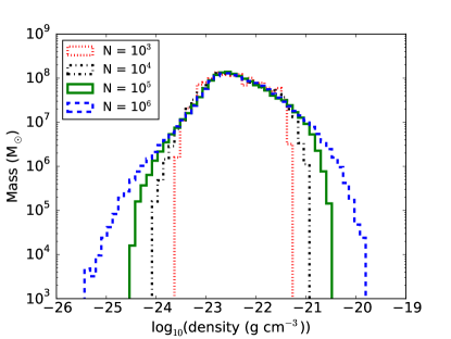
Figure 1: Gas density distribution at 1 Myr for simulations with $10^{3}$ (red), $10^{4}$ (black), $10^{5}$ (green) and $10^{6}$ (blue) particles. Both the high and the low density tails of the gas density distribution are better resolved as the mass resolution of the simulation is improved.

Before investigating how the feedback interacts with the ISM we compare the properties of the ISM itself at different resolutions. Figure 1 shows the density distribution for the gas, at different resolutions, after 1 Myr i.e. just before the feedback turns on. At this point in the simulation the gas distribution is identical for all of the runs at the same resolution, e.g. the blue curve in the figure is the same for the runs FN6c, FN6h, FM6c and FM6h. Figure 1 shows that the lowest resolution runs, with $10^{3}$ particles, probe a much narrower density range than the runs in which $10^{6}$ particles are used. The highest resolution runs thus resolve the density distribution tails at both the low and high density ends. This means that with improved resolution we are able to better distinguish the high and low density phases of the ISM, which, as we show below, can have a large impact on the efficiency of AGN feedback.

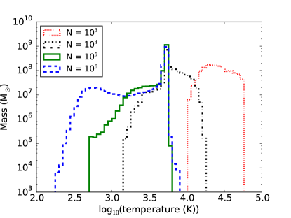
Figure 2: Gas temperature distribution at 1 Myr for simulations with $10^{3}$ (red), $10^{4}$ (black), $10^{5}$ (green) and $10^{6}$ (blue) particles. The low-temperature (dense) gas is completely unresolved in the low resolution simulations.

Figure 2 shows the temperature distribution for the gas, at different resolutions, after 1 Myr. In this figure we can see that in the lowest resolution simulations ($10^{3}$ particles) the gas remains warm, $T>10^{4}$ K. This is due to the dynamical temperature floor that we employ (which is a common approach in cosmological and galaxy formation simulations, see text after equation 3). As the mass resolution is increased the gas can cool to progressively lower temperatures. It can also be seen that in simulations with $10^{5}$ and $10^{6}$ particles the maximum temperature of the gas (before any AGN feedback is initiated) converges to $T\sim 10^{3.7}$ K. The reason for this is that at lower temperatures ($T\lower 2.15277pt\hbox{$\;\buildrel<\over{\sim}\;$}10^{4}$ K) the gas cools much slower, so that there tends to be a lot of gas “piling up” at $T\sim 10^{4}$ K.

3.2 Overview of numerical resolution trends

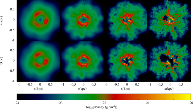
Figure 3: Density slices at $y=0$ through simulation domains at 1.5 Myr. The top row shows runs FM3h, FM4h, FM5h and FM6h from left to right respectively while the FN3h, FN4h, FN5h and FN6h runs are shown from left to right respectively on the bottom row.

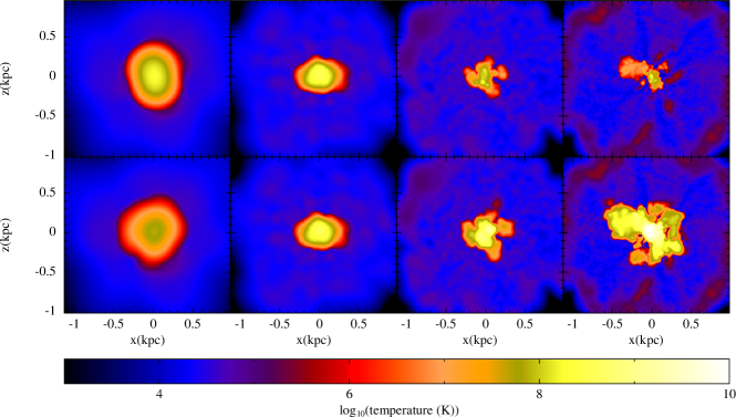
Figure 4: Temperature slices at $y=0$ through simulation domain showing gas temperature at 1.5 Myr. The top row shows runs FM3h, FM4h, FM5h and FM6h from left to right respectively while the FN3h, FN4h, FN5h and FN6h runs are shown from left to right respectively on the bottom row.

Figure 3 shows rendered images of gas density slices through the simulation domain at $y=0$ after $1.5$ Myr. The top row shows the FM3h, FM4h, FM5h and FM6h runs from left to right respectively while the bottom row shows the FN3h, FN4h, FN5h and FN6h runs from left to right respectively. The figure clearly illustrates the increasing complexity of structure that can be resolved with improved resolution. In the low resolution runs (left panels) there is a fairly symmetrical swept-up shell of high density gas, while the high resolution runs (right panels) consist of compressed high density filaments and cleared low density channels through which hot gas can escape.

Figure 4 shows the respective temperature slices. At low resolution (left panels) the feedback outflow sweeps up essentially everything in its path, with no cold gas left at small radii, whilst the hot gas is contained in the central regions only. In contrast, in the higher resolution runs (right panels) the cold gas is still present in clumps and filaments at small radii, whereas the heated gas escapes through low density channels and is now more spatially extended. Since it is likely that the cold gas is the source of efficient SMBH growth, these results show that not only SMBH feedback but also SMBH growth is affected by the numerical resolution artefacts i.e. at low resolution there is a lack of high density cold gas clumps.

The simulations also show stark differences in gas thermodynamical properties between the runs in which the feedback is coupled to a fixed mass (the FM series of runs) versus those with a fixed neighbour number (the FN series of simulations). For instance, due to the differences in the feedback implementation, in FN6h (bottom right panels of figures 3 and 4) a factor $\sim 100$ times less mass is heated than in FM6h (top right panels of figures 3 and 4) and hence the gas is heated to much higher temperatures in FN6h than in FM6h. This results in the feedback in FN6h being more effective at clearing gas from the central region. However there is still cold, dense, in-flowing gas present at small radii.

3.3 Impact of feedback on the ISM

3.3.1 Resolving the ISM density structure

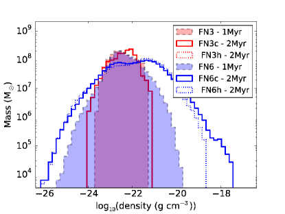
Figure 5: Comparison of gas density distributions at 1 Myr (filled) and 2 Myr (not filled) for FN3 (red) and FN6 (blue) runs with and without IC cooling (solid and dotted respectively). It is clear to see that in the FN3 runs the density distribution changes very little, while in the FN6 runs the gas can be compressed to considerably higher densities.

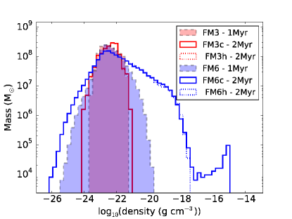
Figure 6: As in figure 5 except for the FM3 and FM6 runs. However, the FM6c run exhibits a particularly high density feature not seen in other runs.

Figure 5 compares the density distribution at 1Myr (filled) and 2Myr (not filled) (i.e. before and after the AGN outburst) for the FN6 (blue) and FN3 (red) runs. In the FN3 runs there is very little evolution in the density distribution with time. However, in the FN6 runs the highest value of gas density reached in the simulation increases by approximately two orders of magnitude, especially when IC cooling is included (compare the dotted and solid lines).

Similar behaviour is seen when comparing the FM3 and FM6 runs in figure 6. The FM6c run exhibits a particularly high density feature not seen in other runs. While the mass in this feature corresponds to only $\sim$ one resolution element, it is interesting to note its existence. The likely cause of this clump is two-fold. Compared with the FM6h run, the gas in the FM6c run can cool via IC processes allowing it to collapse to higher densities. Furthermore, comparing with the FN6 runs, the gas heated directly by the AGN feedback does not reach such high temperatures in the FM6 runs, potentially resulting in cooler clumps that can reach higher densities.

In the higher resolution runs the AGN feedback is able to compress gas to much higher densities, which could result in triggered star formation (e.g. Elbaz et al., 2009; Gaibler et al., 2012; Nayakshin & Zubovas, 2012; Silk, 2013; Zubovas et al., 2013a; Cresci et al., 2015). The figure demonstrates that compression of the ISM into high density features is largely missed in the low resolution runs probably because the ISM structure is under-resolved.

3.3.2 Resolving outflows and inflows

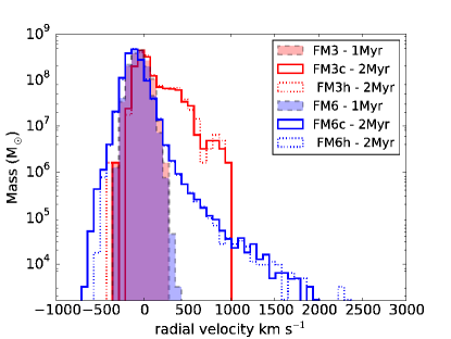
Figure 7: Comparison of radial velocity distributions at 1 Myr (filled) and 2 Myr (not filled) for FM3 (red) and FM6 (blue) runs with and without IC cooling (solid and dotted respectively). Both high and low resolution runs produce gas out-flowing with velocities of order $1000$ km s^-1, however the high resolution runs (FM6) show far stronger gas inflows than the low resolution runs (FM3).

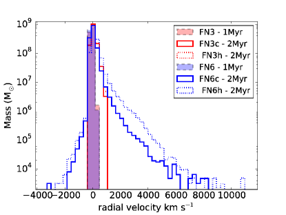
Figure 8: As in figure 7 except for the FN3 and FN6 runs. Due to the significantly higher temperatures reached in the FN6 runs, compared to the FM6 runs, the gas outflows can reach much higher velocities.

The radial velocity of gas in the simulations is also affected by numerical resolution. Contrasting the FM3 and FM6 runs, figure 7 shows that whilst both high and low resolution runs produce gas out-flowing with velocities of order $1000$ km s^-1, the same cannot be said about the in-flowing gas: the high resolution runs (FM6) show far stronger gas inflows than the low resolution runs (FM3). The same behaviour is found when comparing the FN3 and FN6 runs in figure 8. It is interesting to note that for this implementation of feedback, the out-flowing gas can reach much higher velocities in the FN6 run than in the FN3 run (by a factor of $\sim 10$). This can be attributed to the much higher temperatures achieved in the FN6 run. The physical reason for the in-flowing gas present only in the high resolution runs is the previously emphasised inability of the low resolution simulations to model the high density features properly. The high density clumps and filaments present at high resolution are artificially smoothed in lower resolution runs. This results in the high density gas being far less resilient to feedback in the low resolution runs and hence being blown away with the rest of the gas. Needless to say, this is a serious artefact as the SMBH may be fed by exactly this high density gas falling into the centre of the galaxy despite the SMBH feedback (e.g., Nayakshin, 2014).

3.4 Efficiency of feedback versus numerics

3.4.1 The over-cooling problem

Supernova feedback simulations show a well known “over-cooling problem” which affects simulation results and is discussed at length in Dalla Vecchia & Schaye (2012). We, like other studies (e.g. Booth & Schaye, 2009; McCarthy et al., 2010, 2011; Le Brun et al., 2014; Schaye et al., 2015; Crain et al., 2015), find that this problem also exists in AGN feedback simulations. The maximum temperature of the gas directly heated by the feedback, that is the SPH neighbours of the SMBH particle in which the feedback energy is directly deposited, is inversely proportional to the total mass of the gas heated. The radiative cooling rate of the gas is a strong function of temperature in certain temperature ranges. Therefore, the impact of radiative cooling on the thermal evolution of this gas depends in a complicated fashion on the number or total mass of SPH particles in which the feedback energy is injected. In low resolution simulations it is likely that the injected energy is spread over an unrealistically large mass of ambient gas. This typically means that this feedback-heated gas cools on timescales much shorter than one would physically expect.

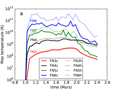
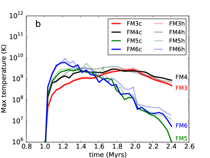
Figure 9: Time evolution of the maximum gas temperature. The top panel (a) shows the FN3 (red), FN4 (black), FN5 (green) and FN6 (blue) runs whilst the bottom panel (b) shows the FM3 (red), FM4 (black), FM5 (green) and FM6 (blue) runs. Solid and dotted lines indicate runs with and without IC cooling.This figure shows that the temperature to which gas is heated to is strongly dependent on the mass of gas heated.

Figure 9 shows the time evolution of the instantaneous maximum gas temperature for simulations in which the feedback energy is injected into a fixed number of SPH particles ($\sim 100$) during each time step (FN3 (red), FN4 (black), FN5 (green) and FN6 (blue)) in the top panel (a) and for simulations in which the feedback energy is injected into a fixed mass ($\sim 1.6\times 10^{7}M_{\odot}$) of gas during each time step (FM3 (red), FM4 (black), FM5 (green) and FM6 (blue)) in the bottom panel (b). The solid and dotted lines show runs with and without IC cooling respectively. Considering first the fixed number of neighbours (FN) runs in the top panel (a), it roughly follows that each order of magnitude improvement in resolution results in an order of magnitude increase in temperature. This is because the feedback energy is injected into a factor $\sim 10$ times less gas mass for each factor $10$ increase in mass resolution.

The fixed mass (FM) runs in the bottom panel (b) lead to more consistent results in that the maximum temperature of gas varies much less between the different resolution simulations, as is expected. However, at later times the higher resolution runs FM5 and FM6 do differ significantly from the lower resolution curves. We believe this is caused by differences in gas properties beyond the immediate feedback deposition region. As we know from figure 3, there is more dense gas near the black hole in the better resolved simulations. This denser gas is hence better at radiating the feedback energy away than in the lower resolution runs.

Finally we note that if included, IC cooling dominates the cooling function at high temperatures for gas close to the SMBH. This explains why the dotted and dashed curves in figure 9 only exhibit differences when gas is heated to high temperatures.

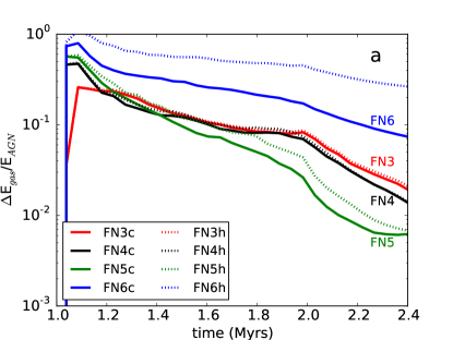
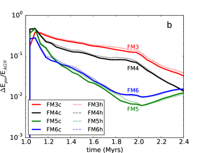
Figure 10: Evolution of the ratio of total gas energy, $E_{\rm gas}$, to total AGN input energy, $E_{\rm AGN}$, from the beginning of the AGN outburst between 1 Myr and 2 Myr. The top panel (a) shows the FN3 (red), FN4 (black), FN5 (green) and FN6 (blue) runs. In this panel there is no apparent trend with resolution. In both panels the solid and dotted lines correspond to runs with and without IC cooling respectively. The bottom panel (b) shows the FM3 (red), FM4 (black), FM5 (green) and FM6 (blue) runs. There is an evident trend that lower resolution runs retain more energy than high resolution runs.

The mode of feedback energy delivery to the ambient gas strongly affects the subsequent evolution of the system. This can be seen in figure 10 which shows the time evolution of the ratio of the change in gas internal and kinetic energy to the energy injected by the AGN as a function of time. As in figure 9, in the top panel (a) the feedback energy is injected into a fixed number of SPH particles ($\sim 100$) during each time step whereas in the bottom panel (b) the feedback energy is injected into a fixed mass ($\sim 1.6\times 10^{7}M_{\odot}$) of gas during each time step. The change in total gas energy at time $t$, $\Delta E_{\rm gas}(t)$, is given as

$$\Delta E_{\rm gas}(t)=E_{\rm gas}(t)-E_{\rm gas}(1{\rm Myr})$$ (9)

where

$$E_{\rm gas}(t)=\sum\limits_{i}\left({\frac{1}{2}m_{\rm i}v_{\rm i}^{2}+\frac{3}{2}\frac{k_{\rm B}T_{\rm i}}{\mu m_{\rm P}}m_{\rm i}}\right)$$ (10)

is the sum of the kinetic and internal energy of all of the SPH particles at time $t$. The total AGN input energy, $E_{\rm AGN}$ is given by

$$E_{\rm AGN}=\epsilon_{\rm f}L_{\rm AGN}t_{\rm act}$$ (11)

where $t_{\rm act}$ is the time for which the AGN has been active. Focusing on the FN series of runs first (top panel, a), we find no clear trend in how much feedback energy is retained by the gas. The two low resolution cases, FN3 and FN4, are rather similar; then the higher resolution case, FN5, retains less energy than that, but the highest resolution case, FN6, retains much more energy than the low resolution cases. We believe that this is due to competition between two somewhat oppositely directed numerical artefacts, one due to the over cooling problem close to the AGN and the other due to poor sampling of the ambient gas farther out. As the resolution is improved, one is able to heat a lower mass of gas and hence heat the gas to higher temperatures, resulting in longer cooling times. However at higher resolution one can resolve high density material which has a shorter cooling time than the lower density material found in the vicinity of the SMBH in lower resolution simulations. Given the competition between the processes contributing to the gas cooling rate there is not necessarily a clear trend in feedback energy conservation with resolution.

The fixed mass runs (FM, the bottom panel, b, of the figure) give a more consistent picture, with FM5 and FM6 yielding very similar results, perhaps indicating that a degree of numerical convergence is taking place. Here we see that at higher resolution less feedback energy is retained in the ambient gas of the galaxy, presumably because higher density clumps are better resolved at higher resolutions and they lead to more energy being lost to radiation. These results show that simulations in which feedback is spread around a fixed mass of ambient gas should be preferred for numerical reasons to those where the number of AGN neighbours is fixed instead. However it should be noted that although injecting feedback energy into a fixed mass of particles provides a degree of numerical convergence, it is not necessarily convergence towards the physically correct result. A further potentially confounding factor is the energy imparted by the momentum of the AGN wind. This is not included in the models presented in this paper, however a purely momentum-driven wind should have a kinetic energy rate $\dot{E}_{\rm mom}\simeq 2\sigma/(\eta c)\dot{E}_{\rm wind}\simeq 0.01\dot{E}_{\rm wind}$. In the high-resolution models, this energy is comparable to the energy retained by the gas and may further complicate gas behaviour. However, a more detailed investigation of the effects of different AGN feedback prescriptions is beyond the scope of this paper.

3.4.2 Gas ejection efficiency

It is believed that the most important effect of AGN feedback onto their host galaxies is to remove gas from the host galaxy and thus quench star formation. In this section we show that the ability of an AGN to clear the gas out of the host is greatly affected by numerical resolution at least for the initial conditions and parameter space investigated in this paper.

To quantify the AGN feedback impact on the host, we first consider the evolution of the total baryonic mass enclosed within 200pc of the host’s centre. We define the fractional change in baryonic mass as

$$\frac{\Delta M_{<200{\rm pc}}(t)}{M_{<200{\rm pc}}(1{\rm Myr})}=\frac{M_{<200{\rm pc}}(t)-M_{<200{\rm pc}}(1{\rm Myr})}{M_{<200{\rm pc}}(1{\rm Myr})}$$ (12)

where $M_{<200{\rm pc}}(t)$ is the total baryonic mass within $200$ pc, including gas accreted onto the black hole but not the initial black hole mass ( $10^{8}{\,{\rm M}_{\odot}}$) itself. Figure 11 shows the time evolution of ${\Delta M_{<200{\rm pc}}(t)}/{M_{<200{\rm pc}}(1{\rm Myr})}$ for simulations with $10^{3}$, $10^{4}$, $10^{5}$ and $10^{6}$ particles shown in black, blue, red and green, respectively. The fixed mass (FM, bottom panel, b) runs show a trend with resolution such that feedback becomes less effective at clearing gas out with improved resolution. The FM3 run which retains the largest fraction of energy is the most effective at clearing gas out, whilst the FM5 and FM6 runs, which lose the most energy, cannot prevent the continual infall of gas. However, if we consider the FN runs (top panel, a) there is no clear trend. Even though the FN6 run retains substantially more energy than the FN3 run, it is far less effective at clearing gas out. This can be attributed to being able to resolve structure in the ISM. As we improve resolution, the hot gas can escape through paths of least resistance leaving higher density clumps behind.

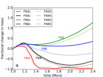
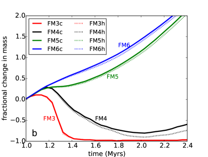
Figure 11: Time evolution of the fractional mass change within the central 200 pc of the system. The top panel (a) shows the FN3 (red), FN4 (black), FN5 (green) and FN6 (blue) runs. As in figure 10 there is no apparent trend with resolution, however, like in the FM runs, the FN3 and FN4 runs are the most efficient at removing gas. The bottom panel (b) shows the FM3 (red), FM4 (black), FM5 (green) and FM6 (blue) runs. As the resolution is degraded the feedback becomes more efficient at clearing gas from the central regions. In both panels the solid and dotted lines correspond to runs with and without IC cooling respectively.

Finally we attempt to further quantify the ability of an AGN to clear gas out by calculating the fraction of gas with radial velocity greater than $2\sigma$. This is shown in figure 12, with the same colour scheme as previous plots. For the FM runs (bottom panel, b) there is a clear trend that as the resolution is improved the fraction of gas out-flowing at a high velocity becomes smaller. However for the FN runs (top panel, a), this trend breaks down for the highest resolution run, FN6. This suggests that the cooling as well as the ability to resolve structure plays an important role in determining how effectively gas can be blown out of the galaxy. As discussed when considering figures 4 and 9 with respect to the FN5 and FN6 runs, the gas in the FN6 runs is heated to higher temperatures than that in the FN5 runs. The cooling in the FN6 runs is less efficient and thus the hot feedback bubble conserves more energy than in the FN5 runs and is able to drive more powerful outflows.

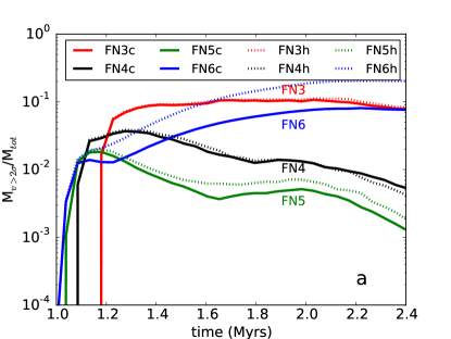
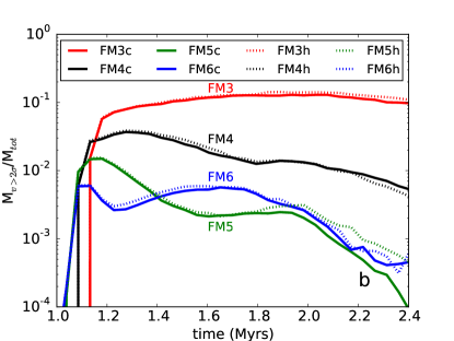
Figure 12: Time evolution of the fraction of gas with radial velocity greater than $2\sigma$. The top panel (a) shows the FN3 (red), FN4 (black), FN5 (green) and FN6 (blue) runs. Again, as in previous figures there is no apparent trend with resolution with both the FN3 and FN6 runs producing outflows containing similar fractions of gas. The bottom panel (b) shows the FM3 (red), FM4 (black), FM5 (green) and FM6 (blue) runs. As in figure 11 there is an apparent trend with resolution, with a greater fraction of gas being out-flowing at a high velocity in the lower resolution runs than in the high resolution runs. In both panels the solid and dotted lines correspond to runs with and without IC cooling respectively.

4 Discussion and summary

We have studied the effect of AGN feedback on a multiphase interstellar medium and how such feedback is affected by numerical resolution. The resolution has two competing effects on the results. Unsurprisingly, the density structure is better resolved at higher resolutions, so that there is more hot low-density and also cold high-density gas than in low resolution simulations. Low resolution simulations thus tend to expel all the gas from the centres of host galaxies, whereas higher resolution simulations do not; they also show dense clumps that are more resilient to feedback and may continue to fall inward while most of the gas is driven out. On the other hand, the over-cooling problem may affect the gas in the immediate vicinity of the SMBH, actually reducing feedback efficiency in low resolution simulations. We now discuss these opposing effects in detail.

4.1 Resolving the multiphase ISM and outflow properties

The inferred properties of outflows in our simulations strongly depend upon the resolution and how the feedback energy is coupled to the ISM. At low resolution the feedback sweeps up all the material in SMBH vicinity into an outflow with a modest velocity ($\sim 1000$ km s^-1). In contrast, at high resolutions only some of the neighbouring gas is launched into the outflow. The outflows can reach higher radial velocities (up to $\sim 5000$ km s^-1); however, cold dense filaments may continue to fall in and feed the SMBH. Higher resolution SPH simulations thus lead to a much more varied outcome for the gas in the galaxy in every measurable quantity, e.g., density, temperature and velocity. This is potentially very important for SMBH growth since even a tiny mass of ambient gas is sufficient to increase the SMBH mass significantly.

In the same vein, cosmological simulations often have to invoke high stellar feedback efficiencies in order to produce observed galactic winds (Schaye et al., 2015). One possible reason for this, in addition to the over-cooling problem, is that low resolution inhibits low density channels through which outflows can escape to reach galactic scales. Alternatively, in some cosmological and galaxy-scale simulations, such winds are hydrodynamically decoupled from the ISM so that they can freely stream to galactic scales (Springel & Hernquist, 2003; Oppenheimer & Davé, 2006; Oppenheimer et al., 2010; Puchwein & Springel, 2013). While such ad-hoc prescriptions allow one to produce realistic outflows at large radii, one loses any information regarding the direct interaction of feedback with the ISM. It is therefore clear that cosmological simulations are unable to provide detailed insights into the feedback mechanisms themselves and the best that one can hope for is that their effects on resolvable scales are modelled correctly.

4.2 Cooling of the feedback bubble

It is evident that the ability of the feedback bubble to conserve its energy has a significant impact on how efficient it is in destroying the host galaxy. This can depend intimately both upon the temperature to which gas is heated directly by the AGN and the processes through which the feedback heated bubble cools. Considering the first point, we have shown that there are stark differences in the properties of the feedback depending upon the mass of the gas heated by AGN feedback. This leads us to the question, what temperature is correct? Analytical theory suggests that wind shocks have temperatures of $10^{10}-10^{11}$ K, however, as illustrated by figure 9, in order to reach such high gas temperatures in a cosmological simulation, a gas mass of $\lower 2.15277pt\hbox{$\;\buildrel<\over{\sim}\;$}1$ SPH particle would need to be heated. Therefore, in such simulations, gas is typically heated to lower temperatures, which could potentially result in incorrect energy conservation in the hot bubble. Such problems may be mitigated to some degree by tuning the efficiency of the feedback or artificially turning off radiative cooling in order to match observations. Whilst such procedures can lead to correct large scale properties of the galaxies, e.g. correct stellar masses and the $M_{\rm BH}-\sigma$ relation, one clearly loses predictive power if observations need to be used to calibrate the models.

With regard to our second point, i.e. the relevance of different cooling mechanisms, the inclusion or absence of IC processes can have a big effect. Comparing the FN6c and FN6h runs, it is clear from figures 10, 11 and 12 that the hot bubble retains more energy and clears out more gas when IC cooling is neglected. It is therefore important to understand which scenario is more physically motivated. Faucher-Giguère & Quataert (2012) have shown that given the high temperature and low density properties of shocked outflows, the electrons and ions are thermally decoupled. The electron cooling timescale is shorter than the electron-ion thermalisation timescale and therefore it is the latter that determines the cooling rate of the gas, with IC cooling becoming ineffective. This suggests that the runs in which IC cooling is neglected are more physically motivated. However, even if the mass and temperature of the feedback bubble matches those expected from analytical theory, the simulated feedback bubble likely has a higher density than the actual shocked wind bubble would, because we are directly heating ISM gas. Therefore the cooling of the hot bubble and its interaction with the ambient ISM may still be incorrectly modelled. Thus we conclude that direct physically self-consistent modelling of AGN feedback heating and cooling on small scales is still beyond the reach of modern numerical capabilities.

4.3 Star formation during an AGN outburst

Figures 5 and 6 clearly show that gas can be compressed to high densities by an AGN outflow. The presence of dense gas can result in additional star formation, which both quantitatively and qualitatively changes the properties of the AGN host galaxy. Similar aspects of AGN-triggered star formation have already been explored by Nayakshin & Zubovas (2012) and Zubovas et al. (2013a), who found that significant star formation can occur both in the cooling out-flowing medium and in the compressed disc of the host galaxy. Our results show that any density contrasts can be enhanced by AGN outflows.

It is important that one needs simulations with sufficient resolution to recover the compression effect in numerical simulations (Figures 5 and 6). Large-scale simulations with low numerical resolution typically miss this effect and hence over-predict the negative (gas removal) effect of AGN feedback. Even in high-resolution simulations, star formation in dense clumps is difficult to track during the AGN outflow if one employs a heating-cooling prescription such as that of Sazonov et al. (2005), which includes Compton heating. This prescription assumes that gas is optically thin, which is a good approximation for the low density ISM, but not for the dense clumps. As a result, the clump temperature, in general, stays too high (i.e. above the temperature set by equation 3) and fragmentation is slower than it would be with a proper radiative transfer treatment.

The lack of AGN-triggered star formation in low-resolution simulations of galaxy evolution presents two challenges: quantitative and qualitative. The quantitative challenge is the issue of reconciling the star formation histories of simulated and observed galaxies. If one channel of triggered star formation is missed in simulations, the other star formation channels have to be proportionately enhanced (for example, by adopting higher star formation efficiencies or lower density thresholds) in order to reproduce the galaxy stellar mass functions of present-day galaxies. The qualitative challenge is arguably more important: AGN outflows create dense star-forming gas where there was none, i.e. affect the location of star-forming regions in the galaxy. This process directly affects the morphology of the starburst and the dynamics of new-born stars (Nayakshin & Zubovas, 2012; Zubovas et al., 2013b). Both of these effects are missed in low-resolution simulations; however, they can be used as strong indicators of positive AGN feedback.

One region where AGN-induced star formation may be particularly important is galaxy centres. These regions typically contain dense gas discs or rings (e.g. Böker et al., 2008), which often show clumpy structures and embedded young star clusters. It is generally accepted that star formation in these regions is induced by shocks caused by matter in-falling via galactic bars from larger radii. However, the presence of young clusters and the lack of azimuthal age gradient in some of these systems complicate this picture (Böker et al., 2008). Another trigger of star formation in these systems could be AGN outflows. As these outflows expand perpendicularly to the disc plane due to lower density (Zubovas & Nayakshin, 2014), they significantly compress the gas in the midplane; in addition, ram pressure of the AGN wind pushes the disc gas into a narrower ring, which is more prone to gravitational instability (Zubovas, submitted). In this way, the density contrast between the disc and its surroundings is also enhanced, much like the density contrast between different regions in the simulations presented in this paper.

4.4 Black hole growth and the $M_{\rm BH}-\sigma$ relation

The general trend in the simulations we present is that at higher resolution less gas is cleared out than at lower resolutions. In low resolution runs the outflow sweeps up everything in its path, creating a sharp cut-off radius between out-flowing material and in-flowing material. However in high resolution runs the outflow only sweeps up low density material, whilst high density material can continue to flow inward. This could lead to very different feeding cycles for the black hole. The supply of material to the black hole is completely cut off and cleared to large radii in the low resolution runs, whereas in the high resolution runs clumps and filaments can remain in-flowing at small radii and thus continuously feed the black hole. This sets up a scenario in which feedback is “all or nothing” at low resolution but more diluted at high resolution, with feeding becoming interminable up to the point that the gas can form stars.

In the high resolution scenario, the high density clumps will only be acted upon by the momentum of the AGN wind (BNH14, Nayakshin, 2014) with the energy escaping through low density channels. By requiring the ram pressure of the AGN outflow to exceed the gravitational force of the bulge acting on all of the clumps along the line of sight from a SMBH and setting a maximum threshold density for the clumps (assumed to be the density at which they undergo star formation) Nayakshin (2014) finds a critical black hole mass in order to clear out the cold gas of

$$M_{\rm crit}\sim 2.2\times 10^{8}{\,{\rm M}_{\odot}}\sigma_{200}^{4}$$ (13)

comparable to the observed $M_{\rm BH}-\sigma$ relations (e.g., Kormendy & Ho, 2013).

4.5 Comparison with previous work

Recent work (Wagner et al., 2013, BNH14) has shown that the structure of the ISM can impact upon the ability of an AGN to clear out gas and hence quench star formation. BNH14 present high-resolution simulations of an UFO impacting upon an inhomogeneous, turbulent medium and find new processes such as energy leakage and separation of energy and mass flows within the ISM. The shocked outflows escape via paths of least resistance, leaving the high density gas, which is difficult to expel, largely intact. Such processes have previously been missed in analytical models and cosmological simulations mainly because the multiphase nature of the ISM is not resolved and has to be implemented as a sub-resolution model. For example Springel & Hernquist (2003) include a sub-grid multiphase model for star formation while Murante et al. (2010) include a non-equilibrium model that includes the three ISM phases for each SPH particle. Unfortunately such methods mean that the intricate structure one expects is washed out due to low resolution.

This work builds on that of BNH14 by implementing a continuous, Eddington limited feedback outburst, rather than a single hot bubble. Furthermore, we have explored the role of IC cooling against the AGN radiation field, which has been highlighted in the literature as a key feature in understanding the impact of UFOs (Faucher-Giguère & Quataert, 2012). This work adds to the growing body of work (e.g. Wagner et al., 2012, 2013; Costa et al., 2014; Gabor & Bournaud, 2014; Zubovas & Nayakshin, 2014, BNH14) highlighting that the AGN environment can be just as important as the AGN feedback mechanism itself when modelling galaxy evolution. In BNH14, the main aim was to understand the physics of the interaction of an outflow with the multiphase ISM, however in this work we have focused more on how resolution can affect this interaction.

The role of the ISM and its impact on AGN feedback has been studied by a number of authors both for feedback in the form of jets (e.g. Wagner et al., 2012) and UFOs (e.g. Wagner et al., 2013, BNH14). Wagner et al. (2012) present high resolution simulations of jet feedback in a clumpy ISM. They found that if the volume filling factor of the clouds is less than $0.1$ then the hot feedback bubble can expand as in the energy driven limit. Clouds smaller than $\sim 25$ pc are destroyed and dispersed, leading them to argue that feedback prescriptions in cosmological simulations should provide a good description of this regime as a source of negative feedback. However if clouds are larger than $\sim 25$ pc they are more resilient to the feedback. In agreement with this work they find that the clouds can be compressed, potentially triggering star formation. Such behaviour is missed in cosmological simulations. Whilst Wagner et al. (2012) suggest a physical setup in which feedback prescriptions in cosmological simulations may produce correct results, we provide a direct comparison of the nature of feedback when simulated at low resolution (similar to cosmological simulations) and up to three orders of magnitude higher resolution. We have found that across such a resolution range there are marked differences in the evolution of the feedback, caused by a combination of effects including the ability to resolve structure and the thermal and physical properties of the hot feedback bubble.

Further work on scales simulating whole galaxies has shown that large scale structure such as a disk (Gabor & Bournaud, 2014) or filaments (Costa et al., 2014) can also reduce the ability of AGN feedback to remove gas from the galaxy. Such structure should be resolved in cosmological simulations, however resolution effects can still impact upon the properties of the feedback. As we have shown, the temperature to which gas is directly heated by feedback as well as its density can affect the cooling and thus the efficiency of the feedback. Given such large differences between the physical properties of hot feedback bubbles in cosmological simulations and those expected in reality we should pose the question when, if ever, such processes can be included in these simulations. Following a Moore’s law approach the number of particles used in cosmological N-body simulations approximately doubles every 16 months. This would suggest that an increase in the mass resolution by 3 orders of magnitude could be achieved in $\sim 13$ years. However, given the fact that algorithms typically scale worse than O(N), and also considering that the silicon chip capacity is limited, this is an extremely optimistic estimate. It is therefore likely that such an improvement in resolution would take much longer to achieve and depends upon the efficiency with which simulators and programmers can harness the power of parallel processing and other technological advances.

4.6 Implications for cosmological simulations

A caveat to the results presented in this paper is that our simulations do not include self-regulation of the AGN feedback, which plays an important role in galaxy evolution. Instead our simulations only model a single, 1 Myr long, Eddington limited AGN feedback event which is not linked to the gas content of the host galaxy. It may therefore be argued that our results on the numerical artefacts in AGN feedback efficiency do not have direct implications for cosmological simulations. In such simulations, the system will undergo multiple feedback events over cosmological timescales. The rate at which a black hole injects energy into the host galaxy ISM is coupled to the gas accretion rate $\dot{m}_{\rm accr}$ through the equation

$$\dot{E}=\epsilon_{\rm BH}(M_{\rm BH},\dot{m}_{\rm accr})\dot{m}_{\rm accr}c^{2}$$ (14)

where $\epsilon_{\rm BH}(M_{\rm BH},\dot{m}_{\rm accr})$ is as defined in the introduction and can be a function of $M_{\rm BH}$ and $\dot{m}_{\rm accr}$. For example Davis & Laor (2011) determined $\epsilon_{\rm r}$ in 80 quasars by using their bolometric luminosities and absolute accretion rates, calculated using thin accretion disk model spectral fits, finding a scaling with $M_{\rm BH}$ such that $\epsilon_{\rm r}=0.089M_{8}^{0.52}$, where $M_{8}$ is $M_{\rm BH}$ in units of $10^{8}$ M_⊙. Often, however, $\epsilon_{\rm BH}(M_{\rm BH},\dot{m}_{\rm accr})$ is set to be a constant for simplicity.

The coupling of the AGN feedback to the gas content of the galaxy through equation 14 leads to self-regulation of the SMBH growth and feedback resulting in the correct $\dot{E}$ such that the feedback driven outflows balance mass inflow. This, therefore, does not uniquely establish $M_{\rm BH}$ but rather the product $\epsilon_{\rm BH}M_{\rm BH}$ (because $\dot{m}_{\rm accr}$ is usually limited to the Eddington accretion rate). To reproduce the observed black hole correlations, one fixes the value of $\epsilon_{\rm BH}$ (e.g., Booth & Schaye, 2009, 2010; Schaye et al., 2015). Further, provided that $\epsilon_{\rm BH}$ is set to a value within a suitable range, the observed SMBH scaling relations can be reproduced despite large differences in resolution and sub-grid prescriptions (e.g., Di Matteo et al., 2005; Springel et al., 2005; Sijacki et al., 2007; Booth & Schaye, 2009; Schaye et al., 2010, 2015), although some fine tuning may be required (see discussion in the introduction). A key element of self-regulation is that the physical properties of the galaxies, such as the stellar mass (e.g. Di Matteo et al., 2005; Springel et al., 2005; Sijacki et al., 2007; Booth & Schaye, 2009, 2010) or AGN driven outflow rates (Schaye et al., 2015) do not depend upon the chosen value of $\epsilon_{\rm BH}$. The result of this is that any dependencies that $\epsilon_{\rm BH}$ has on resolution whould not effect the global properties of the galaxy due to self-regulation, although may lead to changes in the SMBH mass.

As an alternative to tuning efficiencies, a number of authors have attempted a more physically constrained approach to AGN feedback, in which $\epsilon_{\rm BH}(M_{\rm BH},\dot{m}_{\rm accr})$ is not a free parameter. For example, we here followed the model of King (2005) in setting $\epsilon_{\rm f}=0.05$. Additionally, there is growing evidence that AGN should undergo separate quasar and radio modes of feedback (e.g., Churazov et al., 2005; Heinz et al., 2005; Croton et al., 2006; Ishibashi et al., 2014) depending on the Eddington ratio, $\dot{m}_{\rm accr}/\dot{M}_{\rm Edd}$, each with differing values for $\epsilon_{\rm f}$. It has also been suggested that $\epsilon_{\rm r}$ depends upon $\dot{m}_{\rm accr}$ (e.g., Narayan & Yi, 1995; Mahadevan, 1997; Ciotti & Ostriker, 2001; Ciotti et al., 2009), with some cosmological simulations already attempting to include this additional physics (e.g., Sijacki et al., 2007, 2015; Vogelsberger et al., 2014). Further, an effect that is not typically taken into account in galaxy formation simulations is that of the black hole spin, which can lead to variations in the radiative efficiency in the range of $0.055<\epsilon_{\rm r}<0.42$.

We believe that the future of the field is in these more physically motivated approaches which would hopefully provide predictions constraining the physics of black hole growth and feedback. Despite our simulations lacking self-regulated AGN feedback our results are still important for such an approach. As discussed in the introduction some fine tuning of sub-grid feedback parameters can still be necessary when changing resolution (e.g., Schaye et al., 2015; Crain et al., 2015), sub-grid ISM models (e.g., Booth & Schaye, 2009) or cooling prescriptions (e.g., Sijacki et al., 2015). When comparing results of simulations with different AGN feedback physics to the observations, one must be acutely aware of numerical artefacts that may skew the interpretation of such comparisons.

Further we note the potential dependence that $\epsilon_{\rm BH}$ has with the spatial resolution of the SMBH surroundings. If a simulation probes this parameter on sub-pc scales, then the factor will determine the efficiency of BH wind production; on pc scales, the factor tells us something about the coupling between the wind and the surrounding ISM (perhaps about the clumpiness of the ISM); on scales of tens or hundreds of pc, the factor also encompasses the thermal effects (mostly cooling, but perhaps also heating by the AGN radiation field) of the gas surrounding the AGN. Therefore simulations with different spatial resolution might be probing different processes which contribute to AGN feedback efficiency. This is an important point to consider when interpreting constrained values of $\epsilon_{\rm BH}$.

5 Summary

In this paper we have studied the effect of an Eddington-limited AGN outburst on a multiphase turbulent ISM, with particular focus on the effects of numerical resolution. In general, at higher numerical resolution, more dense clumps and also voids through which the feedback can escape are found. This reduces the efficiency with which AGN feedback clears out the host’s gas. At low resolution this behaviour is lost as the feedback sweeps up essentially all the gas in its path. Additionally, depending on uncertain physical detail of the radiative cooling function for the gas heated by AGN feedback, numerical resolution also affects the amount of AGN feedback energy lost to radiation, and it is not possible to say whether it will increase or decrease the feedback efficiency in a general case. It is therefore plausible that resolution dependent effects alter the efficiency of AGN feedback in such a way that it is difficult to attach solid physical meaning to constrained values of $\epsilon_{\rm BH}=\epsilon_{\rm f}\epsilon_{\rm r}$. We also note that although over cosmological timescales self-regulation results in consistent galaxy properties and outflow rates irrespective of the chosen feedback efficiency, our simulations illustrate certain physical processes, such as energy leakage through a clumpy ISM, that can only be modelled at sufficiently high resolution. Finally, in agreement with Schaye et al. (2015), we therefore suggest caution when trying to “invert” the results of cosmological simulations (usually tuned to fit observations) to learn about certain physical aspects of AGN feeding and feedback.

References

- Bautista et al. (2010) Bautista M. A., Dunn J. P., Arav N., Korista K. T., Moe M., Benn C., 2010, ApJ, 713, 25
- Böker et al. (2008) Böker T., Falcón-Barroso J., Schinnerer E., Knapen J. H., Ryder S., 2008, AJ, 135, 479
- Booth & Schaye (2009) Booth C. M., Schaye J., 2009, MNRAS, 398, 53
- Booth & Schaye (2010) Booth C. M., Schaye J., 2010, MNRAS, 405, L1
- Bourne & Nayakshin (2013) Bourne M. A., Nayakshin S., 2013, MNRAS, 436, 2346
- Bourne et al. (2014) Bourne M. A., Nayakshin S., Hobbs A., 2014, MNRAS, 441, 3055
- Bower et al. (2006) Bower R. G., Benson A. J., Malbon R., et al., 2006, MNRAS, 370, 645
- Cano-Díaz et al. (2012) Cano-Díaz M., Maiolino R., Marconi A., Netzer H., Shemmer O., Cresci G., 2012, A&A, 537, L8
- Churazov et al. (2005) Churazov E., Sazonov S., Sunyaev R., Forman W., Jones C., Böhringer H., 2005, MNRAS, 363, L91
- Cicone et al. (2015) Cicone C., Maiolino R., Gallerani S., et al., 2015, A&A, 574, A14
- Cicone et al. (2014) Cicone C., Maiolino R., Sturm E., et al., 2014, A&A, 562, A21
- Ciotti & Ostriker (2001) Ciotti L., Ostriker J. P., 2001, ApJ, 551, 131
- Ciotti et al. (2009) Ciotti L., Ostriker J. P., Proga D., 2009, ApJ, 699, 89
- Costa et al. (2014) Costa T., Sijacki D., Haehnelt M. G., 2014, MNRAS, 444, 2355
- Crain et al. (2015) Crain R. A., Schaye J., Bower R. G., et al., 2015, MNRAS, 450, 1937
- Cresci et al. (2015) Cresci G., Mainieri V., Brusa M., et al., 2015, ApJ, 799, 82
- Croton et al. (2006) Croton D. J., Springel V., White S. D. M., et al., 2006, MNRAS, 365, 11
- Dalla Vecchia & Schaye (2012) Dalla Vecchia C., Schaye J., 2012, MNRAS, 426, 140
- Davis & Laor (2011) Davis S. W., Laor A., 2011, ApJ, 728, 98
- Dehnen & Aly (2012) Dehnen W., Aly H., 2012, MNRAS, 425, 1068
- Di Matteo et al. (2005) Di Matteo T., Springel V., Hernquist L., 2005, Nature, 433, 604
- Dubinski et al. (1995) Dubinski J., Narayan R., Phillips T. G., 1995, ApJ, 448, 226
- Dubois et al. (2012) Dubois Y., Devriendt J., Slyz A., Teyssier R., 2012, MNRAS, 420, 2662
- Dunn et al. (2010) Dunn J. P., Bautista M., Arav N., et al., 2010, ApJ, 709, 611
- Elbaz et al. (2009) Elbaz D., Jahnke K., Pantin E., Le Borgne D., Letawe G., 2009, A&A, 507, 1359
- Fabian (2012) Fabian A. C., 2012, ARA&A, 50, 455
- Fabjan et al. (2010) Fabjan D., Borgani S., Tornatore L., Saro A., Murante G., Dolag K., 2010, MNRAS, 401, 1670
- Fanidakis et al. (2012) Fanidakis N., Baugh C. M., Benson A. J., et al., 2012, MNRAS, 419, 2797
- Faucher-Giguère & Quataert (2012) Faucher-Giguère C.-A., Quataert E., 2012, MNRAS, 425, 605
- Faucher-Giguère et al. (2012) Faucher-Giguère C.-A., Quataert E., Murray N., 2012, MNRAS, 420, 1347
- Ferrarese & Merritt (2000) Ferrarese L., Merritt D., 2000, ApJL, 539, L9
- Feruglio et al. (2010) Feruglio C., Maiolino R., Piconcelli E., et al., 2010, A&A, 518, L155
- Gabor & Bournaud (2014) Gabor J. M., Bournaud F., 2014, MNRAS, 441, 1615
- Gaibler et al. (2012) Gaibler V., Khochfar S., Krause M., Silk J., 2012, MNRAS, 425, 438
- Gebhardt et al. (2000) Gebhardt K., Bender R., Bower G., et al., 2000, ApJL, 539, L13
- Genzel et al. (2014) Genzel R., Förster Schreiber N. M., Rosario D., et al., 2014, ApJ, 796, 7
- Heinz et al. (2005) Heinz S., Merloni A., Di Matteo T., Sunyaev R., 2005, Ap&SS, 300, 15
- Hobbs et al. (2011) Hobbs A., Nayakshin S., Power C., King A., 2011, MNRAS, 413, 2633
- Hobbs et al. (2013) Hobbs A., Read J., Power C., Cole D., 2013, MNRAS, 434, 1849
- Ishibashi et al. (2014) Ishibashi W., Auger M. W., Zhang D., Fabian A. C., 2014, MNRAS, 443, 1339
- Katz (1992) Katz N., 1992, ApJ, 391, 502
- King (2003) King A., 2003, ApJL, 596, L27
- King (2005) King A., 2005, ApJL, 635, L121
- King & Pounds (2015) King A., Pounds K., 2015, Annual Review of Astronomy and Astrophysics, 53, 1, null
- Kormendy & Ho (2013) Kormendy J., Ho L. C., 2013, ARA&A, 51, 511
- Le Brun et al. (2014) Le Brun A. M. C., McCarthy I. G., Schaye J., Ponman T. J., 2014, MNRAS, 441, 1270
- Mahadevan (1997) Mahadevan R., 1997, ApJ, 477, 585
- Maiolino et al. (2012) Maiolino R., Gallerani S., Neri R., et al., 2012, MNRAS, 425, L66
- Mashchenko et al. (2008) Mashchenko S., Wadsley J., Couchman H. M. P., 2008, Science, 319, 174
- McCarthy et al. (2011) McCarthy I. G., Schaye J., Bower R. G., et al., 2011, MNRAS, 412, 1965
- McCarthy et al. (2010) McCarthy I. G., Schaye J., Ponman T. J., et al., 2010, MNRAS, 406, 822
- McNamara & Nulsen (2007) McNamara B. R., Nulsen P. E. J., 2007, ARA&A, 45, 117
- Murante et al. (2010) Murante G., Monaco P., Giovalli M., Borgani S., Diaferio A., 2010, MNRAS, 405, 1491
- Narayan & Yi (1995) Narayan R., Yi I., 1995, ApJ, 452, 710
- Nayakshin (2014) Nayakshin S., 2014, MNRAS, 437, 2404
- Nayakshin & Zubovas (2012) Nayakshin S., Zubovas K., 2012, MNRAS, 427, 372
- Oppenheimer & Davé (2006) Oppenheimer B. D., Davé R., 2006, MNRAS, 373, 1265
- Oppenheimer et al. (2010) Oppenheimer B. D., Davé R., Kereš D., et al., 2010, MNRAS, 406, 2325
- Planelles et al. (2013) Planelles S., Borgani S., Dolag K., et al., 2013, MNRAS, 431, 1487
- Price (2007) Price D. J., 2007, PASA, 24, 159
- Puchwein & Springel (2013) Puchwein E., Springel V., 2013, MNRAS, 428, 2966
- Read & Hayfield (2012) Read J. I., Hayfield T., 2012, MNRAS, 422, 3037
- Read et al. (2010) Read J. I., Hayfield T., Agertz O., 2010, MNRAS, 405, 1513
- Robertson & Kravtsov (2008) Robertson B. E., Kravtsov A. V., 2008, ApJ, 680, 1083
- Rupke & Veilleux (2011) Rupke D. S. N., Veilleux S., 2011, ApJL, 729, L27
- Sazonov et al. (2005) Sazonov S. Y., Ostriker J. P., Ciotti L., Sunyaev R. A., 2005, MNRAS, 358, 168
- Schaye et al. (2015) Schaye J., Crain R. A., Bower R. G., et al., 2015, MNRAS, 446, 521
- Schaye & Dalla Vecchia (2008) Schaye J., Dalla Vecchia C., 2008, MNRAS, 383, 1210
- Schaye et al. (2010) Schaye J., Dalla Vecchia C., Booth C. M., et al., 2010, MNRAS, 402, 1536
- Sijacki et al. (2007) Sijacki D., Springel V., Di Matteo T., Hernquist L., 2007, MNRAS, 380, 877
- Sijacki et al. (2015) Sijacki D., Vogelsberger M., Genel S., et al., 2015, MNRAS, 452, 575
- Silk (2013) Silk J., 2013, ApJ, 772, 112
- Springel (2005) Springel V., 2005, MNRAS, 364, 1105
- Springel et al. (2005) Springel V., Di Matteo T., Hernquist L., 2005, MNRAS, 361, 776
- Springel & Hernquist (2003) Springel V., Hernquist L., 2003, MNRAS, 339, 289
- Sturm et al. (2011) Sturm E., González-Alfonso E., Veilleux S., et al., 2011, ApJL, 733, L16
- Tombesi et al. (2010a) Tombesi F., Cappi M., Reeves J. N., et al., 2010a, A&A, 521, A57+
- Tombesi et al. (2015) Tombesi F., Meléndez M., Veilleux S., Reeves J. N., González-Alfonso E., Reynolds C. S., 2015, Nature, 519, 436
- Tombesi et al. (2010b) Tombesi F., Sambruna R. M., Reeves J. N., et al., 2010b, ApJ, 719, 700
- Tremaine et al. (2002) Tremaine S., Gebhardt K., Bender R., et al., 2002, ApJ, 574, 740
- Vogelsberger et al. (2014) Vogelsberger M., Genel S., Springel V., et al., 2014, MNRAS, 444, 1518
- Wagner et al. (2012) Wagner A. Y., Bicknell G. V., Umemura M., 2012, ApJ, 757, 136
- Wagner et al. (2013) Wagner A. Y., Umemura M., Bicknell G. V., 2013, ApJL, 763, L18
- Wendland (1995) Wendland H., 1995, Advances in computational Mathematics, 4, 1, 389
- Zubovas & King (2012) Zubovas K., King A., 2012, ApJL, 745, L34
- Zubovas & Nayakshin (2014) Zubovas K., Nayakshin S., 2014, MNRAS, 440, 2625
- Zubovas et al. (2013a) Zubovas K., Nayakshin S., King A., Wilkinson M., 2013a, MNRAS, 433, 3079
- Zubovas et al. (2013b) Zubovas K., Nayakshin S., Sazonov S., Sunyaev R., 2013b, MNRAS, 431, 793