Consistent Basis Pursuit for Signal and Matrix Estimates
in Quantized Compressed Sensing

Abstract

This paper focuses on the estimation of low-complexity signals when they are observed through $M$ uniformly quantized compressive observations. Among such signals, we consider 1-D sparse vectors, low-rank matrices, or compressible signals that are well approximated by one of these two models. In this context, we prove the estimation efficiency of a variant of Basis Pursuit Denoise, called Consistent Basis Pursuit (CoBP), enforcing consistency between the observations and the re-observed estimate, while promoting its low-complexity nature. We show that the reconstruction error of CoBP decays like $M^{-1/4}$ when all parameters but $M$ are fixed. Our proof is connected to recent bounds on the proximity of vectors or matrices when (i) those belong to a set of small intrinsic “dimension”, as measured by the Gaussian mean width, and (ii) they share the same quantized (dithered) random projections. By solving CoBP with a proximal algorithm, we provide some extensive numerical observations that confirm the theoretical bound as $M$ is increased, displaying even faster error decay than predicted. The same phenomenon is observed in the special, yet important case of 1-bit CS.
 
Keywords: Quantized compressed sensing, quantization, consistency, error decay, low-rank, sparsity.

1 Introduction

The theory of Compressed Sensing (CS) shows that many signals of interest can be reconstructed from a few linear, and typically random, observations [6, 16, 17]. Interestingly, this reconstruction is made possible if the number of observations (or measurements) is adjusted to the intrinsic complexity of the signal, e.g., its sparsity for vectors or its low-rankness for matrices. Thus, this principle is a generalization of the Shannon-Nyquist sampling theorem, where the sampling rate is set by the bandwidth of the signal. However, a significant aspect of CS systems is the effect of quantization on the acquired observations, in particular for the purpose of compression and transmission [5, 21, 27, 22, 37, 13, 14]. This quantization is a non-linear transformation that both distorts the CS observations and increases, especially at low bit rates, the reconstruction error of CS reconstruction procedures.

This work focuses on minimizing the impact of (scalar) quantization during the reconstruction of a signal from its quantized compressive observations. While more efficient quantization procedures exist in the literature (e.g., $\Sigma\Delta$ [21], universal [3], binned [30, 27], vector [30, 29] or analysis-by-synthesis quantizations [34]), scalar quantization remains appealing for its implementation simplicity in most electronic devices, and for its robustness against measurement lost.

Conversely to other attempts, which consider quantization distortion as additive Gaussian measurement noise [8] and promote a Euclidean ($\ell_{2}$) fidelity with the signal observations as in the Basis Pursuit Denoise (BPDN) program, better signal reconstruction methods are reached by forcing consistency between the re-observed signal estimate and the quantized observations [27, 35, 19].

We show here that a consistent version of the basis pursuit program [11], coined CoBP, provides better signal estimates at large $M$ than those obtained by BPDN. When reconstructing sparse or compressible signals, CoBP is similar, up to an additional normalization constraint, to former methods proposed in [13, 14, 22, 15]. We prove the efficiency of CoBP from recent results on the proximity of signals when those are taken in a set $\mathcal{K}\subset\mathbb{R}^{N}$ of small “dimension”, i.e., with small Gaussian width $w(\mathcal{K})$ [1, 10], and when their quantized random projections are consistent [24, 25]. In particular, we show that for sub-Gaussian sensing matrices, the $\ell_{2}$-reconstruction error of CoBP decays as $\nicefrac{{\sqrt{w(\mathcal{K})}}}{{M^{1/4}}}$, with an additional constant error bias arising in the case of non-Gaussian sensing matrices. This contrasts with BPDN, whose reconstruction error is only guaranteed to saturate when $M$ increases.

The rest of this paper is structured as follows. Sec. 2 introduces the problem by explaining the low-complexity signal space, our Quantized Compressed Sensing (QCS) model and the BPDN reconstruction procedure as generally used in QCS. Sec. 3 reviews important results on the proximity of consistent vectors; in Sec. 4 we introduce and analyze CoBP. Finally, Sec. 5 demonstrates experimentally the capabilities of this method in QCS of signals and matrices, before concluding.

Conventions: Vectors and matrices are associated to bold symbols. The probability of an event $\mathcal{X}$ is $\mathbb{P}(\mathcal{X})$. The identity matrix is $\operatorname{\mathds{1}}_{D}\in\mathbb{R}^{D\times D}$ ($D\in\mathbb{N}$), ${[\![D]\!]}:=\{1,\,\cdots,D\}$ and $|\mathcal{S}|$ is the cardinality of $\mathcal{S}\subset{[\![D]\!]}$. The $\ell_{p}$-norm of $\boldsymbol{u}$ is $\|\boldsymbol{u}\|_{p}$ and the unit $\ell_{p}$-ball is $\mathbb{B}_{p}^{N}=\{\boldsymbol{x}\in\mathbb{R}^{N}:\|\boldsymbol{x}\|_{p}\leqslant 1\}$, with $\mathbb{B}^{N}:=\mathbb{B}_{2}^{N}$. Assuming $N=n^{2}$ is a square number, for a matrix $\boldsymbol{U}=(\boldsymbol{u}_{1},\,\cdots,\boldsymbol{u}_{n})\in\mathbb{R}^{n\times n}$ with vectorization $\operatorname{vec}(\boldsymbol{U}):=(\boldsymbol{u}^{T}_{1},\,\cdots,\boldsymbol{u}^{T}_{n})^{T}\in\mathbb{R}^{N}$, $\operatorname{rank}(\boldsymbol{U})$, $\|\boldsymbol{U}\|$, $\|\boldsymbol{U}\|_{*}$ and $\|\boldsymbol{U}\|_{F}:=\operatorname{tr}(\boldsymbol{U}^{T}\boldsymbol{U})^{1/2}=\|\!\operatorname{vec}(\boldsymbol{U})\|_{2}$ denote its rank, operator norm, nuclear norm and its Frobenius norm, respectively. We will often assimilate matrices in $\mathbb{R}^{n\times n}$ with their vectorization in $\mathbb{R}^{N}$, e.g., identifying $\{\boldsymbol{U}\in\mathbb{R}^{n\times n}:\|\boldsymbol{U}\|_{F}\leqslant 1\}$ with $\mathbb{B}^{N}$. Finally, we write $f\lesssim g$ or $f=O(g)$ if $f\leqslant c\,g$ for $c>0$, and similarly for $f\gtrsim g$ and $f=\Omega(g)$.

2 Quantized Compressed Sensing of Low-Complexity Signals

2.1 Low-complexity Signal Model

This work focuses on the sensing of signals belonging to a low-complexity set $\mathcal{K}\subset\mathbb{R}^{N}$. A typical example is the set of $K$-sparse vectors $\mathcal{K}=\Sigma_{K}:=\{\boldsymbol{u}\in\mathbb{R}^{N}:\|\boldsymbol{u}\|_{0}:=|{\rm supp}\,\boldsymbol{u}|\leqslant K\}$, as well as the set of rank-$r$ matrices $\mathcal{C}_{r}:=\{\boldsymbol{U}\in\mathbb{R}^{n\times n}\simeq\mathbb{R}^{N}:\operatorname{rank}(\boldsymbol{U})\leqslant r\}$.

As in [10], we assume that the (bounded) convex hull $\overline{\mathcal{K}}:=\operatorname{conv}({\mathcal{K}\cap\mathbb{B}^{N}})$ of $\mathcal{K}$ is associated to the definition of an appropriate atomic norm ${\|\!\cdot\!\|_{\sharp}}$ such that

$$\overline{\mathcal{K}}=\overline{\mathcal{K}}_{s}:=\{\boldsymbol{u}\in\mathbb{R}^{N}:\|\boldsymbol{u}\|_{\sharp}\leqslant s,\|\boldsymbol{u}\|_{2}\leqslant 1\},$$ (1)

for some $s>0$. For instance, for compressible signals in $\overline{\Sigma}_{K}$, ${\|\!\cdot\!\|_{\sharp}}={\|\!\cdot\!\|_{1}}$ and $s=\sqrt{K}$, while for matrices in $\overline{\mathcal{C}}_{r}$, ${\|\!\cdot\!\|_{\sharp}}={\|\!\cdot\!\|_{\ast}}$ for $s=\sqrt{r}$ [32].

The “low-complexity” nature of these sets stems from their small Gaussian mean width

$$w(\mathcal{K}):=\mathbb{E}\sup_{\boldsymbol{u}\in\mathcal{K}}|\boldsymbol{g}^{T}\boldsymbol{u}|,\quad\boldsymbol{g}\sim\mathcal{N}(0,\operatorname{\mathds{1}}_{N}).$$

For instance, $w(\Sigma_{K})^{2}=w(\overline{\Sigma}_{K})^{2}\lesssim K\log\nicefrac{{N}}{{K}}$ and $w(\mathcal{C}_{r})^{2}=w(\overline{\mathcal{C}_{r}})^{2}\leqslant 4nr$ [1, 10]. The quantity $w(\mathcal{K})$, also called Gaussian complexity, has been recognized as central, e.g., for random processes characterization [36], high-dimensional statistics and inverse problem solving [9, 10] or classification in randomly projected domains [2]. As explained below, $w(\mathcal{K})$ also determines the minimal number of measurements for CS of signals in $\mathcal{K}$ [10].

2.2 Quantized Compressed Sensing

Given a certain quantization resolution $\delta>0$, we focus on the impact of a uniform (midrise) quantizer $\mathcal{Q}(t):=\delta(\lfloor\tfrac{t}{\delta}\rfloor+\frac{1}{2})\in\mathbb{Z}_{\delta}:=\delta(\mathbb{Z}+\frac{1}{2})$, applied componentwise, in the quantized sensing model

$$\boldsymbol{q}={\boldsymbol{A}}(\boldsymbol{x}_{0}):=\mathcal{Q}(\boldsymbol{\Phi}\boldsymbol{x}_{0}+\boldsymbol{\xi})\in\mathbb{Z}^{M}_{\delta},$$ (2)

where $\boldsymbol{\Phi}\in\mathbb{R}^{M\times N}$ is a random sensing matrix and $\boldsymbol{\xi}\sim\mathcal{U}^{M}([-\delta/2,\delta/2])$ (i.e., $\xi_{i}\sim_{\rm iid}\mathcal{U}([-\delta/2,\delta/2])$ for $i\in{[\![M]\!]}$) is a uniform dithering. This random dithering is known at the signal reconstruction and stabilizes the action of $\mathcal{Q}$ [3, 20, 23]. By slightly abusing the notation, when (2) senses an element $\boldsymbol{X}_{0}$ of a matrix set in $\mathbb{R}^{n\times n}$, $\boldsymbol{x}_{0}=\operatorname{vec}(\boldsymbol{X}_{0})$ amounts to the $N$-length vectorization of this element, assuming $N=n^{2}$.

As often the case in CS, we consider that $\boldsymbol{\Phi}$ is a sub-Gaussian random matrix, i.e., its entries are distributed as $\Phi_{ij}\sim_{\rm iid}\varphi$ with $\varphi$ a symmetric, zero-mean and unit-variance sub-Gaussian random variable (r.v.), having finite sub-Gaussian norm

$$\textstyle\|\varphi\|_{\psi_{2}}:=\sup_{p\geqslant 1}p^{-1/2}(\mathbb{E}|\varphi|^{p})^{1/p}<\infty.$$

For such a r.v. of sub-Gaussian norm $\alpha>0$, we have in fact $\mathbb{P}[|\varphi|>t]\lesssim\exp(-ct^{2}/\alpha^{2})$ for any $t>0$. Examples of such r.v.’s are Gaussian, uniform, bounded or Bernoulli distributed r.v.’s. Below, we write $\varphi\sim\mathcal{N}_{{\rm sg},\alpha}(0,1)$, and the shorthand $\boldsymbol{\Phi}\sim\mathcal{N}_{{\rm sg},\alpha}^{M\times N}(0,1)$ for the associated $M\times N$ matrix, to specify that $\varphi$ is a sub-Gaussian r.v. of norm $\alpha$.

In the absence of quantization, if $M\gtrsim w(\mathcal{K})^{2}$, with high probability, any $\boldsymbol{x}_{0}\in\mathcal{K}$ can be reconstructed from sub-Gaussian observations $\boldsymbol{\Phi}\boldsymbol{x}_{0}$ using convex optimization programs such as Basis Pursuit [10]. Therefore, the minimal number of measurements needed for reconstructing $K$-sparse or compressible signals in $\mathbb{R}^{N}$ grows like $K\log\nicefrac{{N}}{{K}}$, and like $nr$ for rank-$r$ and compressible $n\times n$ matrices [1, 10].

1-bit Quantization Regime:

The exponentially decaying tail bounds of the sub-Gaussian entries of $\boldsymbol{\Phi}$ show that a suitable value of $\delta$ can essentially turn (2) into a 1-bit CS model when $\mathcal{K}$ is bounded [26, 33, 4]. Indeed, from the definition of $\mathcal{Q}$ and assuming $\|\boldsymbol{x}_{0}\|_{2}=1$, for $i\in{[\![M]\!]}$, $\mathbb{P}[q_{i}\notin\{\pm\delta/2\}]=\mathbb{P}[|\boldsymbol{\varphi}_{i}^{T}\boldsymbol{x}+\xi_{i}|\geqslant\delta]=p_{0}\leqslant 2\exp(-{\textstyle\frac{1}{2}}\delta^{2})$, with $p_{0}=0.0027$ for $\delta=3$. Our study holds in such a regime with the interesting advantage of allowing the estimation of the signal norm, as opposed to the 1-bit CS model ${\rm sign}\,(\boldsymbol{\Phi}\boldsymbol{x}_{0})$ [4, 32]. This is due to the pre-quantization dithering in (2). Interestingly, combining the sign operator with prequantization thresholds in 1-bit CS also removes this signal norm uncertainty [28].

2.3 Basis Pursuit Denoise

The first method used to estimate $\boldsymbol{x}_{0}$ from $\boldsymbol{q}$ in (2) was considering quantization as an additive noise of bounded power under high resolution assumption (HRA), i.e., $\delta\ll\|\boldsymbol{x}_{0}\|_{2}$ [6]. In (2), the impact of the dithering provides $\boldsymbol{q}=(\boldsymbol{\Phi}\boldsymbol{x}+\boldsymbol{\xi})+\boldsymbol{n}$ with $\boldsymbol{n}:=\boldsymbol{q}-(\boldsymbol{\Phi}\boldsymbol{x}+\boldsymbol{\xi})\sim\mathcal{U}^{M}([-\delta/2,\delta/2])$. Therefore, $\|\boldsymbol{n}\|_{2}^{2}\leqslant\epsilon^{2}=M\frac{\delta^{2}}{12}+\kappa\sqrt{M}$ holds with high probability for small $\kappa$ (e.g., $\kappa=2$) [22, 20]. In such a case, the general BPDN program,

$$\boldsymbol{x}^{*}_{\rm BPDN}:=\operatorname*{argmin}_{\boldsymbol{u}\in\mathbb{R}^{N}}\|\boldsymbol{u}\|_{\sharp}\ \operatorname{{s.\!t.}}\ \|\boldsymbol{\Phi}\boldsymbol{u}+\boldsymbol{\xi}-\boldsymbol{q}\|_{2}\leqslant\epsilon$$ (BPDN)

can be solved for estimating $\boldsymbol{x}_{0}$. When $\nicefrac{{\boldsymbol{\Phi}}}{{\sqrt{M}}}$ satisfies the restricted isometry property (RIP) and when $\mathcal{K}$ is the set of sparse signals, then, setting ${\|\!\cdot\!\|_{\sharp}}={\|\!\cdot\!\|_{1}}$, [21, 22] show that

$$\|\boldsymbol{x}^{*}-\boldsymbol{x}_{0}\|_{2}=O(\nicefrac{{\epsilon}}{{\sqrt{M}}})=O(\delta).$$

A similar result holds in the case of QCS of low-rank matrices using a Lasso reconstruction that minimizes a Lagrangian formulation of BPDN [7]. Notice that a variant of BPDN, called Basis Pursuit DeQuantizer of moment $p$ (BPDQ [22]), replaces the $\ell_{2}$-norm of the BPDN constraint by an $\ell_{p}$-norm ($2\leqslant p<\infty$). Its error decays like $O(\delta/\sqrt{\log M})$ [5].

3 Proximity of Consistent Vectors

This section summarizes a recent study showing that the proximity of vectors of a subset $\mathcal{K}\subset\mathbb{R}^{N}$ with small Gaussian mean width can be bounded provided they share the same image through the random mapping ${\boldsymbol{A}}$, i.e., if they are consistent [25]. As will be clear in Sec. 4, this property is the key for characterizing the behavior of CoBP.

This proximity is impacted by the level of anisotropy of the sub-Gaussian rows composing $\boldsymbol{\Phi}\sim\mathcal{N}_{{\rm sg},\alpha}^{M\times N}(0,1)$ [1], as measured by the smallest $\kappa_{{}_{{}^{\rm sg}}}\geqslant 0$ such that, for $\boldsymbol{\varphi}\sim\mathcal{N}_{{\rm sg},\alpha}^{N}(0,1)$, $\boldsymbol{g}\sim\mathcal{N}^{N}(0,1)$ and all $\boldsymbol{u}\in\mathbb{R}^{N}$,

$$\!\!\textstyle\int_{0}^{+\infty}\big{|}\mathbb{P}(|\langle\boldsymbol{\varphi},\boldsymbol{u}\rangle|\geqslant t)-\mathbb{P}(|\langle\boldsymbol{g},\boldsymbol{u}\rangle|\geqslant t)\big{|}\,\mathrm{d}t\,\leqslant\,\kappa_{{}_{{}^{\rm sg}}}\|\boldsymbol{u}\|_{\infty}.$$ (3)

For Gaussian (isotropic) random vectors $\kappa_{{}_{{}^{\rm sg}}}=0$, while for sub-Gaussian $\boldsymbol{\varphi}\sim\mathcal{N}_{{\rm sg},\alpha}^{N}(0,1)$, $\kappa_{{}_{{}^{\rm sg}}}\leqslant 9\sqrt{27}\,\alpha^{3}$, with $\alpha\leqslant 1$ for Bernoulli r.v.’s [25].

As clarified in Prop. 1, when the mapping ${\boldsymbol{A}}$ integrates a non-Gaussian, but sub-Gaussian sensing matrix $\boldsymbol{\Phi}$, the proximity of consistent elements $\boldsymbol{x},\boldsymbol{y}$ in $\mathcal{K}$ is guaranteed when $\boldsymbol{x}-\boldsymbol{y}$ is not “too sparse”, i.e., when it belongs to

$$\text{\reflectbox{$\Sigma$}}_{K_{0}}:=\{\boldsymbol{u}\in\mathbb{R}^{N}:K_{0}\|\boldsymbol{u}\|^{2}_{\infty}\leqslant\|\boldsymbol{u}\|_{2}^{2}\},$$

for $K_{0}$ large enough compared to $\kappa_{{}_{{}^{\rm sg}}}^{2}$. For instance, a $K$-sparse vector $\boldsymbol{u}\in\Sigma_{K}:=\{\boldsymbol{v}:\|\boldsymbol{v}\|_{0}:=|{\rm supp}\,\boldsymbol{v}|\leqslant K\}$ cannot belong to $\text{\reflectbox{$\Sigma$}}_{K_{0}}$ for $K_{0}>K$ as then $\|\boldsymbol{u}\|_{2}^{2}\leqslant K\|\boldsymbol{u}\|^{2}_{\infty}$.

Proposition 1 (Consistency width [25]).

Given a quantization resolution $\delta>0$, $\epsilon\in(0,1)$, a sub-Gaussian distribution $\mathcal{N}_{{\rm sg},\alpha}(0,1)$ respecting (3) for $0\leqslant\kappa_{{}_{{}^{\rm sg}}}<\infty$, and $\mathcal{K}\subset\mathbb{B}^{N}$ a bounded subset of $\mathbb{R}^{N}$, there exist some values $C,c>0$ depending only on $\alpha$ and such that, if

$$M\geqslant C\,\tfrac{(2+\delta)^{4}}{\delta^{2}\epsilon^{4}}\,w(\mathcal{K})^{2},$$ (4)

then, for $\boldsymbol{\Phi}\sim\mathcal{N}_{{\rm sg},\alpha}^{M\times N}(0,1)$, $\boldsymbol{\xi}\sim\mathcal{U}^{M}([-\delta/2,\delta/2])$ and $\sqrt{K}_{0}\geqslant 16\kappa_{{}_{{}^{\rm sg}}}$, with probability exceeding $1-2\exp(-c\epsilon M/(1+\delta))$, we have for all $\boldsymbol{x},\boldsymbol{y}\in\mathcal{K}$

$$\boldsymbol{x}-\boldsymbol{y}\in\text{\reflectbox{$\Sigma$}}_{K_{0}},\ {\boldsymbol{A}}(\boldsymbol{x})={\boldsymbol{A}}(\boldsymbol{y})\quad\Rightarrow\quad\|\boldsymbol{x}-\boldsymbol{y}\|_{2}\leqslant\epsilon,$$ (5)

with ${\boldsymbol{A}}$ defined in (2). Moreover, for any orthonormal basis $\boldsymbol{\Psi}\in\mathbb{R}^{N\times N}$, if $\mathcal{K}=(\boldsymbol{\Psi}\Sigma_{K})\cap\mathbb{B}^{N}$ then (4) simplifies to

$$M\geqslant C^{\prime}\,\tfrac{2+\delta}{\epsilon}\,K\log\big{(}\tfrac{N}{K\delta}(\tfrac{2+\delta}{\epsilon})^{3/2}\big{)},$$ (6)

for some $C^{\prime}>0$ depending only on $\alpha$.

We remark that for Gaussian sensing matrices, the “antisparse” condition on $\boldsymbol{x}-\boldsymbol{y}$ (and on $K_{0}$) vanishes since $\kappa_{{}_{{}^{\rm sg}}}=0$. This provides, in the special case of the sparse signal set, a proximity bound in (5) formerly established in [24].

4 Consistent Basis Pursuit

The previous sections allow us now to define a suitable reconstruction procedure for estimating any signal $\boldsymbol{x}_{0}\in\overline{\mathcal{K}}_{s}$ (for some $s>0$ in (1)) observed through the model (2), e.g., for reconstructing compressible signals or matrices belonging to $\overline{\Sigma}_{K}$ or $\overline{\mathcal{C}}_{r}$, respectively. We split the study according to the nature of the sensing matrix.

4.1 Gaussian Sensing Matrix

When $\boldsymbol{\Phi}$ is Gaussian, i.e., $\kappa_{{}_{{}^{\rm sg}}}=0$, we propose to estimate $\boldsymbol{x}_{0}$ with the following program coined Consistent Basis Pursuit,

$$\boldsymbol{x}^{*}:=\operatorname*{argmin}_{\boldsymbol{u}\in\mathbb{R}^{N}}\|\boldsymbol{u}\|_{\sharp}\ \operatorname{{s.\!t.}}\ {\boldsymbol{A}}(\boldsymbol{u})={\boldsymbol{A}}(\boldsymbol{x}_{0}),\ \boldsymbol{u}\in\mathbb{B}^{N}.$$ (CoBP)

This is a convex optimization as the first constraint is equivalent to $\|\boldsymbol{\Phi}\boldsymbol{u}+\boldsymbol{\xi}-{\boldsymbol{A}}(\boldsymbol{x}_{0})\|_{\infty}\leqslant\delta/2$ [22]. The proximity of $\boldsymbol{x}^{*}$ to $\boldsymbol{x}_{0}$ is then guaranteed by Prop. 1.

Proposition 2.

If ${\boldsymbol{A}}$ respects (5) for all $\boldsymbol{x},\boldsymbol{y}\in\overline{\mathcal{K}}_{s}$ and $K_{0}=0$, then for all $\boldsymbol{x}_{0}\in\overline{\mathcal{K}}$, the estimate $\boldsymbol{x}^{*}$ obtained by CoBP from $\boldsymbol{q}={\boldsymbol{A}}(\boldsymbol{x}_{0})$ satisfies $\|\boldsymbol{x}_{0}-\boldsymbol{x}^{*}\|_{2}\leqslant\epsilon$.

Proof.

Since $\boldsymbol{x}_{0}\in\overline{\mathcal{K}}_{s}$ is a feasible vector of the CoBP constraints, we necessarily have $\|\boldsymbol{x}^{*}\|_{\sharp}\leqslant\|\boldsymbol{x}_{0}\|_{\sharp}\leqslant s$. By definition of CoBP, $\boldsymbol{x}^{*}\in\mathbb{B}^{N}$ so that $\boldsymbol{x}^{*}\in\overline{\mathcal{K}}_{s}$. The result follows from (5) with $\boldsymbol{x}=\boldsymbol{x}_{0}$ and $\boldsymbol{y}=\boldsymbol{x}^{*}$. ∎

Prop. 2 assumes that $K_{0}=0$ in (5). This holds if $\kappa_{{}_{{}^{\rm sg}}}=0$, e.g., if $\boldsymbol{\Phi}\sim\mathcal{N}^{M\times N}(0,1)$. Therefore, combining the conditions of Prop. 1 with this last proposition, we get the following corollary by saturating (4) with respect to $M$.

Corollary 1.

Given some universal constant $c>0$, with probability exceeding $1-2\exp(-cM^{3/4}/\sqrt{\delta})$ over the draw of $\boldsymbol{\Phi}\sim\mathcal{N}^{M\times N}(0,1)$ and $\boldsymbol{\xi}\sim\mathcal{U}^{M}([-\delta/2,\delta/2])$, for every $\boldsymbol{x}_{0}\in\overline{\mathcal{K}}_{s}$, the estimate $\boldsymbol{x}^{*}$ obtained by CoBP from $\boldsymbol{q}={\boldsymbol{A}}(\boldsymbol{x}_{0})$ satisfies

$$\textstyle\|\boldsymbol{x}_{0}-\boldsymbol{x}^{*}\|_{2}=O\big{(}\frac{2+\delta}{\sqrt{\delta}}\,(\tfrac{w(\overline{\mathcal{K}}_{s})^{2}}{M})^{1/4}\big{)},$$

i.e., $\|\boldsymbol{x}_{0}-\boldsymbol{x}^{*}\|_{2}=O\big{(}M^{-1/4}\big{)}$ if only $M$ varies.

At first sight, the error decay of CoBP in $M^{-1/4}$ could seem slow. However, as mentioned in Sec. 2.3, the best known error decay for BPDN under the sensing model (2) is $O(\delta)$ [21], which does not decay with $M$. The same constant bound was found for a variant of CoBP without the ball constraint [15].

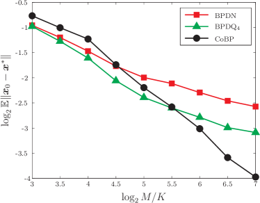
(a) Gaussian QCS of sparse signals.

(b) Bernoulli vs Gaussian QCS of sparse signals.

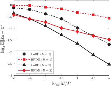
(c) Gaussian QCS of rank-1 matrices.

4.2 Non-Gaussian Sensing Matrix

For non-Gaussian $\boldsymbol{\Phi}$, $\kappa_{{}_{{}^{\rm sg}}}\neq 0$ in general. In order to reach a meaningful estimate of $\boldsymbol{x}_{0}\in\overline{\mathcal{K}}_{s}$, we further assume that $\|\boldsymbol{x}_{0}\|_{\infty}\leqslant\lambda$, for some $\lambda>0$. As will be clear, this allows us to characterize the sparse nature of $\boldsymbol{x}_{0}-\boldsymbol{x}^{*}$ when $\boldsymbol{x}^{*}$ is an estimate of $\boldsymbol{x}_{0}$ produced by the modified program:

$$\boldsymbol{x}^{*}:=\operatorname*{argmin}_{\boldsymbol{u}\in\mathbb{R}^{N}}\|\boldsymbol{u}\|_{\sharp}\ \operatorname{{s.\!t.}}\ \begin{cases}{\boldsymbol{A}}(\boldsymbol{u})={\boldsymbol{A}}(\boldsymbol{x}_{0}),\\ \boldsymbol{u}\in\mathbb{B}^{N}\cap\lambda\mathbb{B}^{N}_{\infty},\end{cases}$$

with ${\bf CoBP}_{\lambda}\equiv{\bf CoBP}$ as soon as $\lambda>1$ since $\mathbb{B}^{N}\subset\mathbb{B}^{N}_{\infty}$.

Proposition 3.

If ${\boldsymbol{A}}$ respects (5) for all $\boldsymbol{x},\boldsymbol{y}\in\overline{\mathcal{K}}_{s}$ and any $K_{0}\geqslant(16\kappa_{{}_{{}^{\rm sg}}})^{2}$, then for any $\boldsymbol{x}_{0}\in\overline{\mathcal{K}}_{s}\cap\lambda\mathbb{B}_{\infty}^{N}$, the solution obtained by CoBP_λ from $\boldsymbol{q}={\boldsymbol{A}}(\boldsymbol{x}_{0})$ respects

$$\|\boldsymbol{x}_{0}-\boldsymbol{x}^{*}\|_{2}\leqslant\epsilon+2\lambda\sqrt{K_{0}}.$$

Proof.

As for the proof of Prop. 2, $\boldsymbol{x}_{0}\in\overline{\mathcal{K}}_{s}$ implies that $\boldsymbol{x}^{*}\in\overline{\mathcal{K}}_{s}$. If $\|\boldsymbol{x}_{0}-\boldsymbol{x}^{*}\|_{2}\leqslant\sqrt{K_{0}}\|\boldsymbol{x}_{0}-\boldsymbol{x}^{*}\|_{\infty}$, then, since $\boldsymbol{x}_{0},\boldsymbol{x}^{*}\in\lambda\mathbb{B}^{N}_{\infty}$, $\|\boldsymbol{x}_{0}-\boldsymbol{x}^{*}\|_{2}\leqslant 2\lambda\sqrt{K_{0}}$. Otherwise, we have $\boldsymbol{x}_{0}-\boldsymbol{x}^{*}\in\text{\reflectbox{$\Sigma$}}_{K_{0}}$. In this case, since (5) is assumed satisfied for all pairs of vectors of $\overline{\mathcal{K}}_{s}$, we have $\|\boldsymbol{x}_{0}-\boldsymbol{x}^{*}\|_{2}\leqslant\epsilon$, which concludes the proof. ∎

Taking $K_{0}=\lceil(16\kappa_{{}_{{}^{\rm sg}}})^{2}\rceil$, this corollary is easily established.

Corollary 2.

Given some universal constant $c>0$, with probability exceeding $1-2\exp(-c\frac{M^{3/4}}{\sqrt{\delta}})$ over the draw of $\boldsymbol{\Phi}\sim\mathcal{N}_{{\rm sg},\alpha}^{M\times N}(0,1)$ and $\boldsymbol{\xi}\sim\mathcal{U}^{M}([-\delta/2,\delta/2])$, the CoBP_λ estimate $\boldsymbol{x}^{*}$ of any $\boldsymbol{x}_{0}\in\overline{\mathcal{K}}_{s}\cap\lambda\mathbb{B}^{N}_{\infty}$ satisfies

$$\textstyle\|\boldsymbol{x}_{0}-\boldsymbol{x}^{*}\|_{2}=O\big{(}\frac{2+\delta}{\sqrt{\delta}}\,(\tfrac{w(\overline{\mathcal{K}}_{s})^{2}}{M})^{1/4}+\kappa_{{}_{{}^{\rm sg}}}\lambda\big{)},$$ (7)

i.e., $\|\boldsymbol{x}_{0}-\boldsymbol{x}^{*}\|_{2}=O(M^{-1/4}+\kappa_{{}_{{}^{\rm sg}}}\lambda)$ if only $M$ varies.

Loosely speaking, Cor. 2 shows that the reconstruction error is not guaranteed to decay below a certain level fixed by $\kappa_{{}_{{}^{\rm sg}}}\|\boldsymbol{x}_{0}\|_{\infty}$. A similar behavior was already observed in the case of 1-bit CS with non-Gaussian measurements  [1].

5 Experiments

In this section we run several numerical simulations in order to assess the experimental benefit of CoBP compared to BPDN in various QCS settings. As CoBP is a convex optimization problem containing non-smooth convex functions, we solve it with the versatile Parallel Proximal Algorithm (PPXA) [12], this one being efficiently implemented in the UNLocBoX toolbox [31]. We refer the reader to [18] for an example application of PPXA in the solution of low-rank matrix recovery.

For our experiments, three different sensing contexts are tested: the two first ones consider QCS of sparse signals (for Gaussian or Bernoulli sensing matrices), while the last one focuses on QCS of rank-1 matrices. In all cases, the quantization resolution is fixed by $\delta=6\times 2^{1-B}$ with $B\in{[\![4]\!]}$. As explained in Sec. 2.2, each $q_{i}$ can then be essentially coded with $B$ bits, e.g., if $B=1$, $\mathbb{E}|\big{\{}i:q_{i}\notin\{\pm\delta/2\}\big{\}}|\leqslant 0.0027M$. Some of our results are compared to those of BPDN with $\epsilon$ set as in Sec. 2.3. The constraint “$\boldsymbol{u}\in\mathbb{B}^{N}$” is also added to BPDN for reaching fair comparisons with CoBP.

5.1 Gaussian QCS of sparse signals

In this experiment, we set $N=2048$, $K=16$, $B=3$ and $M/K\in[8,128]$, i.e., well after the phase transition (here around $M/K\simeq 6$) where sparse signal reconstruction from noisy CS measurements is guaranteed [8]. For each value of $M$, 20 different Gaussian sensing matrices, dithering realizations and unit-norm $K$-sparse signals were randomly generated. Each signal $\boldsymbol{x}_{0}$ has its $K$-length support selected uniformly at random in ${[\![N]\!]}$, with non-zero components drawn as $\mathcal{N}(0,1)$ before normalization. The reconstruction error decay averaged over these 20 trials is shown for BPDN, BPDQ with $p=4$ (see Sec. 2.3) and CoBP in Fig. 1(c)(left) in a $\log_{2}/\log_{2}$ plot. For indication, a linear fitting over the last 4 values of $\log_{2}M/K$ provides slopes of value $-0.31$, $-0.33$ and $-0.95$ for BPDN, BPDQ and CoBP, respectively. As already observed experimentally in other works forcing tight or approximate consistency in signal reconstruction [27, 19, 13, 14, 22], this clearly highlights the advantage of consistent signal reconstruction when $M/K$ is large. Moreover, CoBP approaches an error decay of $M^{-1}$ similar to the distance decay of consistent $K$-sparse vectors when (6) is saturated, i.e., better than the “$M^{-1/4}$” of Cor. 1.

5.2 Bernoulli vs Gaussian QCS

This second experiment stresses the impact of the sub-Gaussian nature of the sensing matrix over the CoBP reconstruction error. We focus on the case of Gaussian QCS ($\boldsymbol{\Phi}\sim\mathcal{N}^{M\times N}(0,1)$) and Bernoulli QCS (i.e., $\Phi_{ij}$ equals $\pm 1$ with probability $1/2$) when observing $K$-sparse signals for $K$ growing and $M/K$ constant. In particular, we set $N=1024$, $B=4$, $K\in[1,64]$ and $M/K=16$. For each value of $K$, 20 different sensing matrices, dithering realizations and unit-norm $K$-sparse signals are generated as in the first experiment. CoBP and CoBP_λ are compared (with an oracle assisted $\lambda:=\|\boldsymbol{x}_{0}\|_{\infty}$). Comparing the error bounds for Gaussian and sub-Gaussian QCS in Cor. 1 and in Cor. 2, respectively, we expect that at low $K$ and for $M/K$ constant, Bernoulli QCS reaches worst reconstruction error than Gaussian QCS, as then the bias $\kappa_{{}_{{}^{\rm sg}}}\lambda=\kappa_{{}_{{}^{\rm sg}}}\|\boldsymbol{x}_{0}\|_{\infty}\simeq\kappa_{{}_{{}^{\rm sg}}}/\sqrt{K}$ can be high. This is indeed observed in Fig. 1(c)(middle) with a clear gap between Bernoulli and Gaussian QCS performances when $K\leqslant 16$. CoBP_λ does lead to clear improvements over CoBP.

5.3 Gaussian QCS of rank-1 matrices

We reconstruct here rank-1 matrices in $\mathbb{R}^{32\times 32}$ (i.e., $N=1024$ and $n=32$) from the Gaussian QCS model (2) with $B\in\{1,2\}$. Both CoBP and BPDN are solved with ${\|\!\cdot\!\|}_{\sharp}={\|\!\cdot\!\|}_{*}$. The intrinsic complexity of such rank-1 matrices is $63<P:=64$. For each value of the oversampling ratio $M/P\in[4,32]$, we generate 20 different Gaussian sensing matrices, dithering realizations and rank-1 matrices according to $\boldsymbol{x}_{0}=\operatorname{vec}(\boldsymbol{X}_{0})$ and $\boldsymbol{X}_{0}=\boldsymbol{v}\boldsymbol{v}^{T}/\|\boldsymbol{v}\|_{2}^{2}$ with $\boldsymbol{v}\sim\mathcal{N}^{n}(0,1)$. As for the first experiment on $K$-sparse signals, CoBP reaches a faster reconstruction error decay than BPDN. At $B=2$, an indicative linear fitting over the last 4 values of $M/K$ provides estimated decay exponents for CoBP and BPDN of $-0.85$ and $-0.33$, respectively.

6 Conclusion

In the context of QCS of signals with low-complexity (e.g., sparse signals, low-rank matrices), we show that the consistent reconstruction method CoBP has an estimation error decaying as $M^{-1/4}$, i.e., faster than the one of BPDN. This is confirmed numerically on several settings with even faster effective decaying rate at quantization resolution as low as one bit per measurement. As observed initially in 1-bit CS [1], QCS performances for general sub-Gaussian sensing matrices are also impacted when the sensed signal is “too sparse”. Finally, to the best of our knowledge, we provided the first theoretical analysis of CoBP in the case of low-rank matrix reconstruction from QCS observations.

References

- [1] A. Ai, A. Lapanowski, Y. Plan, R. Vershynin. One-bit compressed sensing with non-gaussian measurements. Linear Algebra and its Applications, 441:222–239, 2014.
- [2] A. S. Bandeira, D. G. Mixon, B. Recht. Compressive classification and the rare eclipse problem. arXiv preprint arXiv:1404.3203, 2014.
- [3] P. T. Boufounos. Universal rate-efficient scalar quantization. IEEE Trans. Inf. Theory, 58(3):1861–1872, 2012.
- [4] P. T. Boufounos, R. G. Baraniuk. 1-bit compressive sensing. In Proc. Conf. Inform. Science and Systems (CISS), Princeton, NJ, 2008.
- [5] P. T. Boufounos, L. Jacques, F. Krahmer, R. Saab. Quantization and compressive sensing. In book ”Compressed Sensing and its Applications”, Springer, 2014.
- [6] E. Candès, J. Romberg, T. Tao. Stable signal recovery from incomplete and inaccurate measurements. Comm. Pure Appl. Math, 59(8):1207–1223, 2006.
- [7] E. Candès, Y. Plan. Tight oracle inequalities for low-rank matrix recovery from a minimal number of noisy random measurements. IEEE Trans. Inf. Theory, 57(4):2342–2359, 2011.
- [8] E. Candes, T. Tao. Near-optimal signal recovery from random projections: Universal encoding strategies? IEEE Trans. Inf. Theory, 52(12):5406–5425, 2006.
- [9] V. Chandrasekaran, M. Jordan. Computational and statistical tradeoffs via convex relaxation. arXiv preprint arXiv:1211.1073, 2012.
- [10] V. Chandrasekaran, B. Recht, P. A. Parrilo, A. S. Willsky. The convex geometry of linear inverse problems. Found. Comp. Math., 12(6):805–849, 2012.
- [11] S. S. Chen, D. L. Donoho, M. A. Saunders. Atomic Decomposition by Basis Pursuit. SIAM Journal on Scientific Computing, 20(1):33–61, 1998.
- [12] P. L. Combettes, J.-C. Pesquet. Proximal splitting methods in signal processing. In Fixed-point algorithms for inverse problems in science and engineering, pp. 185–212. Springer, 2011.
- [13] W. Dai, H. V. Pham, O. Milenkovic. Distortion-Rate Functions for Quantized Compressive Sensing. In IEEE Inf. Th. Workshop (ITW), pp.171-175, Volos, Greece, June 2009.
- [14] W. Dai, O. Milenkovic, Information theoretical and algorithmic approaches to quantized compressive sensing. IEEE Trans. Comm, 59(7):1857–1866, 2011.
- [15] S. Dirksen, G. Lecué, H. Rauhut. On the gap between RIP-properties and sparse recovery conditions. arXiv preprint arXiv:1504.05073, 2015.
- [16] D. L. Donoho. Compressed Sensing. IEEE Trans. Inf. Theory, 52(4):1289–1306, 2006.
- [17] S. Foucart, H. Rauhut. A mathematical introduction to compressive sensing. Springer, 2013.
- [18] M. Golbabaee, P. Vandergheynst. Hyperspectral image compressed sensing via low-rank and joint-sparse matrix recovery. In IEEE Int. Conf. Ac. Sp. Sig. Proc. (ICASSP), pp. 2741–2744. 2012.
- [19] V. K Goyal, M. Vetterli, N. T. Thao. Quantized overcomplete expansions in : Analysis, synthesis, and algorithms. IEEE Trans. Inf. Theory, 44(1):16–31, 1998.
- [20] R. M. Gray, D. L. Neuhoff. Quantization. IEEE Trans. Inf. Theory, 44(6):2325–2383, 1998.
- [21] C. S. Güntürk, M. Lammers, A. M. Powell, R. Saab, Ö. Yılmaz. Sobolev duals for random frames and quantization of compressed sensing measurements. Found. Comp. Math., 13(1):1–36, 2013.
- [22] L. Jacques, D. K. Hammond, M. J. Fadili. Dequantizing Compressed Sensing: When Oversampling and Non-Gaussian Constraints Combine. IEEE Trans. Inf. Theory, 57(1):559–571, January 2011.
- [23] L. Jacques. A Quantized Johnson Lindenstrauss Lemma: The Finding of Buffon’s Needle. IEEE Trans. Inf. Theory, in press. arXiv preprint arXiv:1309.1507, 2013.
- [24] L. Jacques. Error Decay of (almost) Consistent Signal Estimations from Quantized Random Gaussian Projections. arXiv preprint arXiv:1406.0022, 2014.
- [25] L. Jacques. Small width, low distortions: quasi-isometric embeddings with quantized sub-Gaussian random projections. arXiv preprint arXiv:1504.06170, 2015.
- [26] L. Jacques, J. N. Laska, P. T. Boufounos, R. G. Baraniuk. Robust 1-bit compressive sensing via binary stable embeddings of sparse vectors. IEEE Trans. Inf. Theory, 59(4):2082–2102, 2013.
- [27] U. S. Kamilov, V. K. Goyal, S. Rangan. Message-passing de-quantization with applications to compressed sensing. IEEE Trans. Sig. Proc., 60(12):6270–6281, 2012.
- [28] K. Knudson, R. Saab, R. Ward. One-bit compressive sensing with norm estimation. arXiv preprint arXiv:1404.6853, 2014.
- [29] H. Q. Nguyen, V. K. Goyal, L. R. Varshney. Frame Permutation Quantization. App. Comp. Harm. An. (ACHA), Nov. 2010.
- [30] R. J. Pai. Nonadaptive lossy encoding of sparse signals. M.eng. thesis, MIT EECS, Cambridge, MA, 2006.
- [31] N. Perraudin, D. Shuman, G. Puy, P. Vandergheynst. UNLocBoX: A Matlab convex optimization toolbox using proximal splitting methods. arXiv preprint arXiv:1402.0779, 2014.
- [32] Y. Plan, R. Vershynin. Robust 1-bit compressed sensing and sparse logistic regression: A convex programming approach. IEEE Trans. Inf. Theory, 59(1):482–494, 2013.
- [33] Y. Plan, R. Vershynin. One-bit compressed sensing by linear programming. Comm. Pur. Appl. Math., 66(8):1275–1297, 2013.
- [34] A. Shirazinia, S. Chatterjee, M. Skoglund, Analysis-by-Synthesis Quantization for Compressed Sensing Measurements. IEEE Trans. Sig. Proc., 61(22):5789–5800, 2013.
- [35] J. Z. Sun, V. K. Goyal. Optimal quantization of random measurements in compressed sensing. In Proc. IEEE Int. Symp. Inf. Th. (ISIT), pp. 6–10, 2009.
- [36] A. W. Vaart, J. A. Wellner. Weak convergence and empirical processes. Springer, 1996.
- [37] A. Zymnis, S. Boyd, E. Candes. Compressed sensing with quantized measurements. IEEE Sig. Proc. Let., 17(2):149–152, 2010.