Strong Consistency of Multivariate Spectral Variance Estimators

Abstract

Markov chain Monte Carlo (MCMC) algorithms are used to estimate features of interest of a distribution. The Monte Carlo error in estimation has an asymptotic normal distribution whose multivariate nature has so far been ignored in the MCMC community. We present a class of multivariate spectral variance estimators for the asymptotic covariance matrix in the Markov chain central limit theorem and provide conditions for strong consistency. We examine the finite sample properties of the multivariate spectral variance estimators and its eigenvalues in the context of a vector autoregressive process of order 1.

1 Introduction

Markov chain Monte Carlo (MCMC) methods are often required for parameter estimation in the statistical models encountered in modern applications. The typical MCMC experiment consists of simulating a Markov chain in order to estimate a vector of quantities, such as moments or quantiles, associated with the target distribution. However, the multivariate nature of the estimation has only rarely been acknowledged in the MCMC literature. We consider the situation where estimation of a vector of means is of interest. Given a multivariate Markov chain central limit theorem (CLT) for the sample mean vector, we show that a class of multivariate spectral variance estimators (MSVEs) are strongly consistent estimators of the covariance matrix in the asymptotic normal distribution. We also establish strong consistency of the eigenvalues of any strongly consistent estimator of the asymptotic covariance matrix.

We know of no other comparable work in the context of MCMC. Kosorok, (2000) did propose estimators of the asymptotic covariance matrix which generalized work in the univariate case by Geyer, (1992). However, these estimators are asymptotically conservative and are based on the properties of reversible Markov chains, an assumption we do not make. There has been a substantial amount of work in the univariate setting. In particular, Atchadé, (2011) and Flegal and Jones, (2010) established strong consistency of certain univariate spectral variance estimators, but the multivariate problem is more complicated and requires much new work. Moreover, our work represents a substantial generalization of the univariate results and requires much weaker conditions on the Markov chain. Thus we also improve the current results in the univariate setting.

We will give a more formal description of the problem studied here. Let $F$ be a probability distribution with support $\mathsf{X}$, equipped with a countably generated $\sigma$-field $\mathcal{B}(\mathsf{X})$ and let $g:\mathsf{X}\to\mathbb{R}^{p}$ be an $F$-integrable function such that

$$\theta:=\text{E}_{F}g=\int_{\mathsf{X}}g(x)\,dF$$

is the $p$-dimensional vector of interest. Note that $\mathsf{X}$ and $\theta$ often have different dimensions. It is common to resort to MCMC methods to estimate $\theta$ when it is difficult to obtain $\theta$ analytically or to produce independent samples from $F$. MCMC is popular because it is straightforward to simulate a Harris ergodic (i.e., aperiodic, $F$-irreducible, and positive Harris recurrent) Markov chain having invariant distribution $F$ (Geyer,, 2011; Liu,, 2008; Robert and Casella,, 2013). Letting $X=\{X_{1},X_{2},X_{3},\dots\}$ denote such a Markov chain, estimation is easy since, for any initial distribution, with probability 1,

$$\theta_{n}:=\dfrac{1}{n}\displaystyle\sum_{t=1}^{n}g(X_{t})\to\theta\quad\text{ as }\quad n\to\infty\;.$$ (1.1)

Of course, for any $n$ there will be an unknown Monte Carlo error in estimation, $\theta_{n}-\theta$, and assessment of this Monte Carlo error is critical to the reliability of the simulation results (Flegal et al.,, 2008; Flegal and Jones,, 2011; Geyer,, 1992; Jones and Hobert,, 2001). However, the multivariate nature of the Monte Carlo error has been largely ignored in the MCMC literature (but see Gong and Flegal,, 2015).

Instead, the primary focus has been on assessing the univariate Monte Carlo error. Let $g^{(i)}$, $\theta_{n}^{(i)}$, and $\theta^{(i)}$, denote the $i$th components of $g$, $\theta_{n}$, and $\theta$, respectively. Then $\theta_{n}^{(i)}-\theta^{(i)}$ is the unknown Monte Carlo error of the $i$th component. The approximate sampling distribution of this error is available via a Markov chain CLT if there exists $0<\sigma^{2}_{i}<\infty$ such that, as $n\to\infty$,

$$\sqrt{n}(\theta_{n}^{(i)}-\theta^{(i)})\stackrel{{\scriptstyle d}}{{\to}}\text{N}(0,\sigma^{2}_{i})\;.$$ (1.2)

(See Jones, (2004) and Roberts and Rosenthal, (2004) for a discussion of the conditions for (1.2).) Due to serial correlation in $X$, $\text{Var}_{F}g^{(i)}\neq\sigma^{2}_{i}$, except in trivial cases. Nevertheless, consistent estimation of $\sigma^{2}_{i}$ is key to constructing asymptotically valid confidence intervals for $\theta^{(i)}$ and hence in assessing the reliability of the simulation results (Flegal and Gong,, 2015; Flegal et al.,, 2008; Glynn and Whitt,, 1992; Jones et al.,, 2006; Jones and Hobert,, 2001). Thus consistent estimation of $\sigma^{2}_{i}$ has received significant attention; Atchadé, (2011), Damerdji, (1991), and Flegal and Jones, (2010) studied spectral variance estimators, Hobert et al., (2002) and Mykland et al., (1995) investigated estimators based on regenerative simulation, and Jones et al., (2006) studied nonoverlapping batch means. Geyer, (1992) introduced asymptotically conservative estimators based on the spectral properties of reversible Markov chains. Doss et al., (2014) considered univariate estimators in the context of estimating quantiles.

In the multivariate setting, the approximate sampling distribution of the Monte Carlo error is available via a Markov chain CLT if there exists a positive definite $p\times p$ matrix $\Sigma$ such that

$$\sqrt{n}(\theta_{n}-\theta)\overset{d}{\to}\text{N}_{p}(0,\Sigma)\quad\text{ as }\quad n\to\infty\;.$$ (1.3)

We consider a class of MSVEs of $\Sigma$ and provide conditions for strong consistency. Our main assumption on the process is the existence of a multivariate strong invariance principle (SIP); that is, we assume that the centered and appropriately scaled partial sum process is similar to a Brownian motion. Specifically, an SIP holds for $\{g(X_{t})\}_{t\geq 1}$ if there exists a $p\times p$ lower triangular matrix $L$ and an increasing function $\psi$ on the integers such that, with probability 1,

$$n(\theta_{n}-\theta)=LB(n)+O(\psi(n))~{}~{}~{}\text{ as }~{}~{}n\to\infty~{},$$

where $B(n)$ denotes a $p$-dimensional standard Brownian motion and $LL^{T}=\Sigma$. If $\psi$ is such that $\psi(n)/\sqrt{n}\to 0$ as $n\to\infty$, the SIP implies a strong law, a CLT, and a functional CLT for $\theta_{n}$. Under moment conditions on $g$, an SIP with $\psi(n)=n^{1/2-\lambda}$ for some $\lambda>0$ holds for polynomially ergodic Markov chains.

There has been a substantial amount of work in the context of MCMC on establishing that Markov chains are at least polynomially ergodic. An incomplete list is given by Acosta et al., (2015), Doss and Hobert, (2010), Fort and Moulines, (2003), Hobert and Geyer, (1998), Jarner and Hansen, (2000), Jarner and Roberts, (2002), Jarner and Roberts, (2007), Johnson and Geyer, (2012), Johnson and Jones, (2015), Jones et al., (2014), Marchev and Hobert, (2004), Petrone et al., (1999), Roberts and Rosenthal, (1999), Roberts and Tweedie, (1996), Rosenthal, (1996), Roy and Hobert, (2007), Tan and Hobert, (2012), Tan et al., (2013), and Tierney, (1994). While establishing that a Markov chain is at least polynomially ergodic can be challenging, it is not the obstacle that it once was.

1.1 Motivating Example

As motivation for the use of multivariate methods, we present a simple Bayesian logistic regression model. For $i=1,\dots,K$, let $Y_{i}$ be a binary response variable. For the $i$th observation let $X_{i}=(x_{i1},x_{i2},\dots,x_{i5})$ be the observed vector of predictors, then

$$Y_{i}|X_{i},\beta\overset{ind}{\sim}\text{Bernoulli}\left(\dfrac{1}{1+e^{-X_{i}\beta}}\right)\,,~{}~{}~{}\text{ and }~{}~{}~{}\beta\sim N_{5}(0,I_{5})\;.$$ (1.4)

The resulting posterior $F$ is intractable and hence MCMC is used to obtain estimates of the regression coefficient, $\beta$. We use the logit dataset in the mcmc R package which contains four predictors and 100 observations. The goal is to estimate the posterior mean of $\beta=(\beta_{0},\beta_{1},\beta_{2},\beta_{3},\beta_{4})^{T}$. Thus $g$ here is the identity function mapping to $\mathbb{R}^{5}$.

To sample from the posterior we use the Polya-Gamma Gibbs sampler of Polson et al., (2013) (see the R package BayesLogit) which was shown to be uniformly ergodic by Choi and Hobert, (2013). Although the chain mixes fairly quickly as seen in the autocorrelation plot for $\beta_{0}$ in Figure 1, the cross-correlation plot between $\beta_{0}$ and $\beta_{2}$ indicates correlation across these components that is ignored by univariate methods. As a result in Figure 2, the multivariate confidence ellipse is oriented along non-standard axes (see Vats et al., (2015) for details on how to construct such confidence regions). The ellipse is compared to two univariate confidence boxes; the smaller uncorrected for multiple testing and the larger corrected for two tests using a Bonferroni correction.

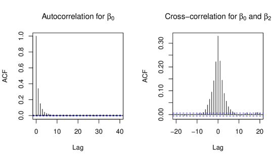
Figure 1: Autocorrelation plot for $\beta_{0}$ and the cross-correlation plot between $\beta_{0}$ and $\beta_{2}$ for a Monte Carlo sample size of $n=10^{5}$.

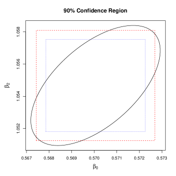
Figure 2: 90% confidence regions constructed using univariate and multivariate methods. The solid ellipse is constructed using an MSVE, the dotted smaller box is constructed using an uncorrected univariate spectral variance estimator and the dashed larger box is constructed using a univariate spectral variance estimator corrected by Bonferroni.

We assess the performance of these confidence regions by comparing their coverage probabilities and volumes over 1000 independent replications for varying Monte Carlo sample sizes. In particular we look at the volume to the $p$th root ($p$ = 5 in this example). The ‘true’ posterior mean is determined by obtaining a Monte Carlo estimate from a sample of length $10^{9}$. Results are presented in Table 1. Note that as the Monte Carlo sample size increases, the multivariate methods produce confidence regions with the nominal coverage probability of $90\%$ with significantly lower volume compared to the Bonferroni corrected regions. The uncorrected regions have far from desirable coverage probabilities.

Table 1: Volume to the $p$th ($p=5$) root and coverage probabilities for 90% confidence regions constructed using MSVE, uncorrected univariate spectral estimators and Bonferroni corrected univariate spectral estimators. Replications = 1000 and standard errors are indicated in parenthesis.

$n$	MSVE	Bonferroni corrected	Uncorrected
Volume to the $5$th root
1e3	0.0574 (4.93e-05)	0.0687 (7.02e-05)	0.0483 (4.93e-05)
1e4	0.0189 (7.50e-06)	0.0226 (1.12e-05)	0.0160 (7.90e-06)
1e5	0.0061 (1.10e-06)	0.0073 (1.50e-06)	0.0051 (1.10e-06)
Coverage Probabilities
1e3	0.853 (0.0112)	0.871 (0.0106)	0.549 (0.0157)
1e4	0.882 (0.0102)	0.904 (0.0093)	0.612 (0.0154)
1e5	0.895 (0.0097)	0.910 (0.0090)	0.602 (0.0155)

One reason for the reduction in volume of the ellipsoid is that multivariate methods capture information ignored by univariate analysis. This also leads to a better understanding of the effective samples obtained in an MCMC sample. Vats et al., (2015) provide the following estimator of effective sample size

$$n\left(\dfrac{|\widehat{\Lambda}|}{|\widehat{\Sigma}|}\right)^{1/p},$$

where $\widehat{\Lambda}$ is the sample covariance matrix for $g(X_{t})$, $\widehat{\Sigma}$ is a strongly consistent estimator of $\Sigma$, and $|\cdot|$ denotes determinant. They demonstrate the superiority of this estimator of effective sample size to the univariate estimator of Kass et al., (1998) and Gong and Flegal, (2015).

The rest of the paper is organized as follows. In Section 2 we formally define the MSVE and present conditions for strong consistency. We also establish strong consistency of the eigenvalues. Section 3 contains a simulation study where we investigate the finite sample properties of the MSVE in the context of a vector autoregressive process. Finally, we present a discussion in Section 4. Many technical details of the proofs from Section 2 are deferred to the appendices.

2 Spectral Estimators and Results

2.1 Definition of MSVE

Let $Y_{t}=g(X_{t})-\theta$, $t=1,2,3,\ldots$ and define the lag $s$, $s\geq 0$, autocovariance matrix as

$$\gamma(s)=\gamma(-s)^{T}=\text{E}_{F}\left[Y_{t}\,Y_{t+s}^{T}\right]\,.$$

Define $I_{s}$ as $I_{s}=\{1,\dots,(n-s)\}$ for $s\geq 0$ and as $I_{s}=\{(1-s),\dots,n\}$ for $s<0$. Let $\bar{Y}_{n}=n^{-1}\sum_{t=1}^{n}Y_{t}$ and define the lag $s$ sample autocovariance as

$$\gamma_{n}(s)=\dfrac{1}{n}\sum_{t\in I_{s}}(Y_{t}-\bar{Y}_{n})(Y_{t+s}-\bar{Y}_{n})^{T}\,.$$ (2.1)

The MSVE is a weighted and truncated sum of the lag $s$ sample autocovariances,

$$\widehat{\Sigma}_{S}=\displaystyle\sum_{s=-(b_{n}-1)}^{b_{n}-1}w_{n}(s)\gamma_{n}(s),$$ (2.2)

where $w_{n}(\cdot)$ is the lag window and $b_{n}$ is the truncation point.

2.2 Strong Consistency of MSVE

2.2.1 Strong Invariance Principle

While Markov chains are our primary interest, we only require $\{X_{t}\}_{t\geq 1}$ to be a stochastic process which satisfies a strong invariance principle or SIP. In the interest of clarity, the SIP was stated somewhat loosely in Section 1. What follows is a formal statement of our assumption.

Recall that $F$ is a distribution having support $\mathsf{X}$, $g:\mathsf{X}\to{\mathbb{R}}^{p}$, and we are interested in estimating $\theta=\text{E}_{F}g$. We assume $g^{2}$ (where the square is element-wise) is an $F$-integrable function. Set $h(X_{t})=\left[g(X_{t})-\theta\right]^{2}$, let $\|\cdot\|$ denote the Euclidean norm, and let $B(t)$ denote a $p$-dimensional standard Brownian motion.

We will require an SIP for the partial sums of both $g$ and $h$. We assume there exists a $p\times p$ lower triangular matrix $L$, an increasing function $\psi$ on the integers, a finite random variable $D$, and a sufficiently rich probability space such that, with probability 1,

$$\left\|\sum_{t=1}^{n}g(X_{t})-n\theta-LB(n)\right\|<D\,\psi(n)\,.$$ (2.3)

We also assume there exists a finite $p$-vector $\theta_{h}$, a $p\times p$ lower triangular matrix $L_{h}$, an increasing function $\psi_{h}$ on the integers, a finite random variable $D_{h}$, and a sufficiently rich probability space such that, with probability 1,

$$\left\|\sum_{t=1}^{n}h(X_{t})-n\theta_{h}-L_{h}B(n)\right\|<D_{h}\,\psi_{h}(n)\,.$$ (2.4)

Remark 1.

Strong invariance principles have attracted much research interest and have been shown to hold for a wide variety of processes; see Section 4 for some discussion on this point. Results from Kuelbs and Philipp, (1980) show that for the Markov chains commonly encountered in MCMC settings, (2.3) and (2.4) hold with $\psi(n)=\psi_{h}(n)=n^{1/2-\lambda}$ for some $\lambda>0$. The correlation of the process is measured indirectly by $\psi$ (Philipp and Stout,, 1975); a large serial correlation implies $\lambda$ is closer to 0 while for less correlated processes $\lambda$ is closer to 1/2.

2.2.2 Strong Consistency

In (2.2) we define the MSVE as the weighted and truncated sum of the lag $s$ sample autocovariances. We make the following assumptions on the lag window $w_{n}(\cdot)$ and the truncation point $b_{n}$.

Condition 1.

The lag window $w_{n}(\cdot)$ is an even function defined on $\mathbb{Z}$ such that

1. $|w_{n}(s)|\leq 1$ for all $n$ and $s$,

2. $w_{n}(0)=1$ for all $n$, and

3. $w_{n}(s)=0$ for all $|s|\geq b_{n}$.

Anderson, (1971) gives a list of lag windows that satisfy Condition 1. We will consider some of these further in Section 2.2.4.

The following Conditions 2 and 3 are technical conditions ensuring that $b_{n}$ grows at the right rate compared to $n$.

Condition 2.

Let $b_{n}$ be an integer sequence such that $b_{n}\to\infty$ and $n/b_{n}\to\infty$ as $n\to\infty$ where $b_{n}$ and $n/b_{n}$ are non-decreasing.

Condition 3.

Let $b_{n}$ be an integer sequence such that

1. there exists a constant $c\geq 1$ such that $\sum_{n}(b_{n}/n)^{c}<\infty$,

2. $b_{n}n^{-1}\log n\to 0$ as $n\to\infty$,

3. $b_{n}^{-1}\log n=O(1)$, and

4. $n>2b_{n}$.

If $b_{n}=\lfloor n^{\nu}\rfloor$, where $0<\nu<1$, then Condition 3 is satisfied if $n>2^{1/(1-\nu)}$.

Define

$$\Delta_{1}w_{n}(k)=w_{n}(k-1)-w_{n}(k)$$

and

$$\Delta_{2}w_{n}(k)=w_{n}(k-1)-2w_{n}(k)+w_{n}(k+1)\;.$$

Condition 4.

Let $b_{n}$ be an integer sequence, $w_{n}$ be the lag window, and $\psi(n)$ and $\psi_{h}(n)$ be positive functions on the integers such that,

1. $b_{n}n^{-1}\sum_{k=1}^{b_{n}}k|\Delta_{1}w_{n}(k)|\to 0$ as $n\to\infty$,

2. $b_{n}\psi(n)^{2}\log n\left(\displaystyle\sum_{k=1}^{b_{n}}|\Delta_{2}w_{n}(k)|\right)^{2}\to 0$ as $n\to\infty$,

3. $\psi(n)^{2}\displaystyle\sum_{k=1}^{b_{n}}|\Delta_{2}w_{n}(k)|\to 0$ as $n\to\infty$,

4. $b_{n}^{-1}\psi_{h}(n)\to 0$ as $n\to\infty$, and

5. $b_{n}^{-1}\psi(n)\to 0$ as $n\to\infty$.

Condition 4a connects the truncation point $b_{n}$ to the lag window $w_{n}$. In Section 2.2.4 we will present examples of lag windows that satisfy this condition. The functions $\psi(n)$ and $\psi_{h}(n)$ in Conditions 4b, 4c, 4d, and 4e correspond to the functions described in (2.3) and (2.4) and thus these four conditions connect the truncation point $b_{n}$, the lag window $w_{n}$, and the correlation of the process, measured indirectly by $\psi(n)$ and $\psi_{h}(n)$. In Lemma 1 we present sufficient conditions for Conditions 4a, 4b, and 4c.

Theorem 1.

Suppose the strong invariance principles (2.3) and (2.4) hold. If Conditions 1, 2, 3, and 4 hold, then $\widehat{\Sigma}_{S}\to\Sigma$, with probability 1, as $n\to\infty$.

Outline of proof.

The proof is split into several lemmas; see Appendix A for details. Define for $l=0,\dots,(n-b_{n})$, $\bar{Y}_{l}(k)=k^{-1}\sum_{t=1}^{k}Y_{l+t}$ and

$$\widehat{\Sigma}_{w,n}=\dfrac{1}{n}\displaystyle\sum_{l=0}^{n-b_{n}}\sum_{k=1}^{b_{n}}k^{2}\Delta_{2}w_{n}(k)[\bar{Y}_{l}(k)-\bar{Y}_{n}][\bar{Y}_{l}(k)-\bar{Y}_{n}]^{T}\,.$$

For $t=1,\dots,n$, define $Z_{t}=Y_{t}-\bar{Y}_{n}$. Then, in Lemma 4 we show that $\widehat{\Sigma}_{w,n}=\widehat{\Sigma}_{S}-d_{n}$, where

$$d_{n} =\dfrac{1}{n}\left\{\sum_{t=1}^{b_{n}}\Delta_{1}w_{n}(t)\left(\sum_{l=1}^{t-1}Z_{l}Z_{l}^{T}+\sum_{l=n-b_{n}+t+1}^{n}Z_{l}Z_{l}^{T}\right)\right.$$

$$\quad\left.+\sum_{s=1}^{b_{n}-1}\left[\sum_{t=1}^{b_{n}-s}\Delta_{1}w_{n}(s+t)\left(\sum_{l=1}^{t-1}\left(Z_{l}Z_{l+s}^{T}+Z_{l+s}Z_{l}^{T}\right)+\sum_{l=n-b_{n}+t+1}^{n-s}\left(Z_{l}Z_{l+s}^{T}+Z_{l+s}Z_{l}^{T}\right)\right)\right]\right\}\;.$$ (2.5)

Notice that in (2.5) we use the convention that empty sums are zero. In Lemma 9 we show that $d_{n}\to 0$ as $n\to\infty$ with probability 1. Thus $\widehat{\Sigma}_{w,n}-\widehat{\Sigma}_{S}\to 0$, with probability 1, as $n\to\infty$. In Lemma 14, we show that $\widehat{\Sigma}_{w,n}\to\Sigma$, with probability 1, as $n\to\infty$, and the result follows. ∎

We use Theorem 1 to give conditions for the strong consistency of $\widehat{\Sigma}_{S}$ when the underlying stochastic process is a Harris ergodic Markov chain having invariant distribution $F$, but first we need a couple of definitions. Recall that $F$ has support $\mathsf{X}$ and $\mathcal{B}(\mathsf{X})$ is a countably generated $\sigma$-field. For $n\in{\mathbb{N}}=\{1,2,3,\ldots\}$, let the $n$-step Markov kernel associated with $X$ starting at $x\in\mathsf{X}$ be $P^{n}(x,dy)$. Then if $A\in\mathcal{B}(\mathsf{X})$ and $r\in\{1,2,3,\ldots\}$, $P^{n}(x,A)=\Pr(X_{r+n}\in A|X_{r}=x)$. Let $\|\cdot\|_{TV}$ denote the total variation norm. The Markov chain is polynomially ergodic of order $\xi$ where $\xi>0$ if there exists $M:\mathsf{X}\to{\mathbb{R}}^{+}$ with $E_{F}M<\infty$ such that

$$\|P^{n}(x,\cdot)-F(\cdot)\|_{TV}\leq M(x)n^{-\xi}\;.$$ (2.6)

Notice that polynomial ergodicity is weaker than geometric or uniform ergodicity; see Meyn and Tweedie, (2009).

Remark 2.

Polynomial ergodicity is often proved by establishing the following drift condition. For a function $V:\mathsf{X}\to[1,\infty)$ there exists $d>0,b<\infty,$ and $0\leq\tau<1$ such that for $x\in\mathsf{X}$

$$E[V(X_{n+1})|X_{n}=x]-V(x)\leq-d[V(x)]^{\tau}+bI(x\in C)\,,$$

where $C$ is a small set. In order to verify that $E_{F}M<\infty$, it is sufficient to show that $E_{F}V<\infty$ by Theorem 14.3.7 in Meyn and Tweedie, (2009).

Theorem 2.

Suppose $\text{E}_{F}\|g\|^{4+\delta}<\infty$ for some $\delta>0$. Let $X$ be a polynomially ergodic Markov chain of order $\xi\geq(1+\epsilon)(1+2/\delta)$ for some $\epsilon>0$. Then (2.3) and (2.4) hold with

$$\psi(n)=\psi_{h}(n)=n^{1/2-\lambda}$$

for some $\lambda>0$ that depends on $p$, $\epsilon$, and $\delta$. If Conditions 1, 2, 3, and 4 hold, then $\widehat{\Sigma}_{S}\to\Sigma$, with probability 1, as $n\to\infty$.

Proof.

See Appendix A.4. ∎

Remark 3.

We rely on results provided by Kuelbs and Philipp, (1980) to establish the existence of (2.3) and (2.4) in Theorem 2. However, the precise relationship of $\lambda$ with $p$, $\epsilon$, and $\delta$ is not investigated in Kuelbs and Philipp, (1980) and remains an open problem.

Remark 4.

When $p=1$, the MSV estimator reduces to the spectral variance estimator (SVE) considered by Atchadé, (2011), Damerdji, (1991), and Flegal and Jones, (2010). However, our result requires weaker conditions. First notice that Flegal and Jones, (2010) required weaker conditions than Damerdji, (1991). Thus we only need to compare Theorem 2 to the results in Atchadé, (2011) and Flegal and Jones, (2010), both of whom required the Markov chains to be geometrically ergodic and to satisfy a one-step minorization condition. Thus Theorem 2 substantially weakens the conditions on the underlying Markov chain, while extending the results to the $p\geq 1$ setting.

2.2.3 Strong Consistency of Eigenvalues

Having obtained a strongly consistent estimator of $\Sigma$, it is natural to consider the eigenvalues of the estimator.

Theorem 3.

Let $\widehat{\Sigma}$ be any strongly consistent estimator of $\Sigma$ and let $\lambda_{1}\geq\lambda_{2}\geq\dots\geq\lambda_{p}>0$ be the eigenvalues of $\Sigma$. Let $\hat{\lambda}_{1},\dots,\hat{\lambda}_{p}$ be the $p$ eigenvalues of $\widehat{\Sigma}$ such that $\hat{\lambda}_{1}\geq\hat{\lambda}_{2}\geq\dots\geq\hat{\lambda}_{p}$, then $\hat{\lambda}_{k}\to\lambda_{k}$, with probability 1, as $n\to\infty$ for all $1\leq k\leq p$.

Proof.

Let $\|\cdot\|_{F}$ denote the Frobenius norm. By Weyl’s inequality (Franklin,, 2012), for $\epsilon>0$, if $\|\widehat{\Sigma}-\Sigma\|_{F}\leq\epsilon$, then for all $1\leq k\leq p$, $|\hat{\lambda}_{k}-\lambda_{k}|\leq\epsilon,$ which gives the desired result. ∎

Remark 5.

Theorem 3 immediately implies that under the conditions of either Theorem 1 or Theorem 2 the sample eigenvalues of the MSVE are consistent for the population eigenvalues. That is, $\hat{\lambda}_{k}\to\lambda_{k}$, with probability 1, as $n\to\infty$ for all $1\leq k\leq p$.

Sample eigenvalues can play an important role in multivariate analyses. For example, the length of any axis of the confidence region constructed from $\widehat{\Sigma}_{S}$ is determined by the magnitude of the relevant estimated sample eigenvalue. Thus the largest eigenvalue is associated with the axis having the largest estimated Monte Carlo error. This also suggests that dimension reduction methods could be useful in assessing the reliability of the simulation effort. Although this is a potentially interesting research direction it is beyond the scope of this paper.

2.2.4 Lag Window Conditions

The following generalization of Lemma 7 in Flegal and Jones, (2010) is useful for checking that a lag window satisfies the conditions of Theorem 1.

Lemma 1.

Reparameterize $w_{n}$ such that $w_{n}$ is defined on $[0,1]$ and $w_{n}(0)=1$ and $w_{n}(1)=0$. Further assume that $w_{n}$ is twice continuously differentiable and that there exists finite constants $D_{1}$ and $D_{2}$ such that $|w_{n}^{\prime}(x)|\leq D_{1}$ and $|w_{n}^{\prime\prime}(x)|<D_{2}$. Then as $n\to\infty$,

1. Condition 4a holds if $b_{n}^{2}n^{-1}\to 0$,

2. Conditions 4b and 4c holds if $b_{n}^{-1}\psi(n)^{2}\log n\to 0$.

Proof.

The argument is the same as that of Lemma 7 in Flegal and Jones, (2010) and hence is omitted. ∎

Remark 6.

It is common to use $b_{n}=\lfloor n^{\nu}\rfloor$ in which case Conditions 4a, 4b, and 4c hold, if we choose $0<\nu<1/2$ such that $n^{-\nu}\psi(n)^{2}\log n\to 0$ as $n\to\infty$.

Remark 7.

We now consider some examples of lag windows which satisfy Condition 1 and consider whether Conditions 4a, 4b, and 4c hold.

1. Simple Truncation: $w_{n}(k)=I(|k|<b_{n})$. Using this window the estimator obtained is truncated at $b_{n}$ but weighted identically. In this case, $\Delta_{2}w_{n}(k)=0$ for $k=1,\dots,b_{n}-2$, $\Delta_{2}w_{n}(b_{n}-1)=-1$ and $\Delta_{2}w_{n}(b_{n})=1$. It is easy to see that Condition 4c is not satisfied.
   

2. Blackman-Tukey: $w_{n}(k)=\left[1-2a+2a\cos\left(\pi|k|/{b_{n}}\right)\right]I(|k|<b_{n})$ where $a>0$. This is a generalization for the Tukey-Hanning window where $a=1/4$. For fixed $a$, the Blackman-Tukey window satisfies the conditions of Lemma 1, thus Conditions 4a, 4b, and 4c hold if $b_{n}^{2}n^{-1}\to 0$ and $b_{n}^{-1}\psi(n)^{2}\log n\to 0$ as $n\to\infty$.
   

3. Parzen: $w_{n}(k)=\left[1-|k|^{q}/{b_{n}^{q}}\right]I(|k|<b_{n})$ for $q\in\mathbb{Z}^{+}$. When $q=1$ this is the modified Bartlett window. It is easy to show that the Parzen window satisfies the conditions for Lemma 1, and thus Conditions 4a, 4b, and 4c hold if $b_{n}^{2}n^{-1}\to 0$ and $b_{n}^{-1}\psi(n)^{2}\log n\to 0$ as $n\to\infty$.
   

4. Scale-parameter modified Bartlett: $w_{n}(k)=\left[1-\eta|k|/{b_{n}}\right]I(|k|<b_{n})$ where $\eta$ is a positive constant not equal to 1. Then $\Delta_{1}w_{n}(k)=\eta b_{n}^{-1}$ for $k=1,2,\dots,b_{n}-1$ and $\Delta_{1}w_{n}(b_{n})=1-\eta+\eta b_{n}^{-1}$ so that Condition 4a is satisfied when $b_{n}^{2}n^{-1}\to 0$ as $n\to\infty$. Also, $\Delta_{2}w_{n}(k)=0$ for $k=1,2,\dots,b_{n}-2$, $\Delta_{2}w_{n}(b_{n}-1)=\eta-1$ and $\Delta_{2}w_{n}(b_{n})=1-\eta+\eta b_{n}^{-1}$. We conclude that $\sum_{k=1}^{b_{n}}|\Delta_{2}w_{n}(k)|$ does not converge to 0 and hence Condition 4c is not satisfied.

Figure 3 provides a graph of the three lag windows we consider in the next section, specifically, the modified Bartlett, Tukey-Hanning, and scale-parameter modified Bartlett windows. It is evident that the modified Bartlett and Tukey-Hanning windows are similar and the scale-parameter modified Bartlett window weighs the lags more severely.

Figure 3: Plot of three lag windows, modified Bartlett (Bartlett), Tukey-Hanning and the scale-parameter Bartlett with scale parameter 2 (Scaled-Bartlett).

3 Simulation

We consider some finite sample properties of the MSVE in the context of a vector autoregressive process of order 1 or VAR(1). Let

$$y_{t}=\Phi y_{t-1}+\epsilon_{t},$$ (3.1)

where $y_{t}\in\mathbb{R}^{p}$ for all $t$, $\Phi$ is a $p\times p$ matrix, $\epsilon_{t}\overset{iid}{\sim}N_{p}(0,W)$, and $y_{0}$ is the zero vector. While this is a simple model, it is useful to study since we can control the correlation of the process.

We assume that the largest eigenvalue of $\Phi$, $\phi_{\max}$, is less than 1 in absolute value, in which case the stationary distribution for the process is $F=N_{p}(0,V)$ where $vec(V)=(I_{p^{2}}-\Phi\otimes\Phi)^{-1}vec(W)$. Here $\otimes$ denotes Kronecker product and $I_{p^{2}}$ is the $p^{2}\times p^{2}$ identity matrix. With some algebra it can be shown that the lag $s$ autocovariance matrix for $s>0$ is

$$\gamma(s)=\Phi^{s}V\,\,\,\,\text{and}\,\,\,\,\gamma(-s)=V(\Phi^{T})^{s}.$$

Consider estimating $\text{E}_{F}y$ with $\bar{y}_{n}$, the Monte Carlo estimate. Tjøstheim, (1990) showed that the process is geometrically ergodic as long as $|\phi_{\max}|<1$. In fact, the smaller the largest eigenvalue, the faster the process mixes. Since $F$ has a moment generating function, a CLT holds with

$$\Sigma =\displaystyle\sum_{s=-\infty}^{\infty}\gamma(s)$$

$$=\displaystyle\sum_{s=0}^{\infty}\gamma(s)+\displaystyle\sum_{s=-\infty}^{0}\gamma(s)-V$$

$$=\displaystyle\sum_{s=0}^{\infty}\Phi^{s}V+\displaystyle\sum_{s=-\infty}^{0}V(\Phi^{T})^{s}-V$$

$$=(1-\Phi)^{-1}V+V\left(1-\Phi^{T}\right)^{-1}-V.$$ (3.2)

For this process, we investigate the performance of the class of MSVE in estimating $\Sigma$. We set $W$ to be the first order autoregressive covariance matrix with correlation $\rho=0.5$ and present simulation results for different settings of $\Phi$ and $p$. These settings are presented in Table 2. For Settings 1 and 4, $\phi_{\max}=.2$, Settings 2 and 5, $\phi_{\max}=.6$ and Settings 3 and 6, $\phi_{\max}=.9$. Thus, these three pairs of settings yield processes with different mixing rates.

Table 2: Simulation settings 1 through 6.

Setting	$p$	Eigenvalues of $\Phi$ for $i=0,\dots,p-1$
1	10	$\lambda_{i}=.01+i(.20-.01)/(p-1)$
2	10	$\lambda_{i}=.40+i(.60-.40)/(p-1)$
3	10	$\lambda_{i}=.70+i(.90-.70)/(p-1)$
4	50	$\lambda_{i}=.01+i(.20-.01)/(p-1)$
5	50	$\lambda_{i}=.40+i(.60-.40)/(p-1)$
6	50	$\lambda_{i}=.70+i(.90-.70)/(p-1)$

We compare the performance of three lag windows: modified Bartlett, Tukey-Hanning, and scale-parameter modified Bartlett with scale $=2$. In Section 2 we showed that the modified Bartlett and the Tukey-Hanning windows satisfy the conditions of Theorem 1 while the scale-parameter modified Bartlett does not.

For each setting, we do the following in each of 100 independent replications. We observe the process for a Monte Carlo sample size of $1e5$, and calculate the three MSVEs at samples $\{1e3,5e3,1e4,5e4,1e5\}$ with $b_{n}=\lfloor n^{1/3}\rfloor$. The error in estimation is determined by calculating the average relative difference in Frobenius norm, i.e. $||\widehat{\Sigma}-\Sigma||_{F}/||\Sigma||_{F}$ for each of the three windows at all five Monte Carlo sample sizes.

In Figure 4, we plot the results for all settings for all three lag windows. For Settings 1 and 4, all three lag windows perform equally well while for Settings 3 and 6, the scale parameter modified Bartlett window performs poorly. In all settings, the modified Bartlett and the Tukey-Hanning windows perform similarly, but the Tukey-Hanning window is slightly better when the chain mixes more slowly. The plots also indicate that as $\phi_{\max}$ increases, a larger Monte Carlo sample size is required for a desired error in estimation threshold. This is as expected since we know for higher values of $\phi_{\max}$, the process mixes more slowly.

Figure 4: $\|\widehat{\Sigma}_{S}-\Sigma\|_{F}/\|\Sigma\|_{F}$ for the three lag windows at different Monte Carlo sample sizes for all six settings averaged over 100 iterations.

In Section 2 we presented the proof for the convergence of the eigenvalues of the MSVE in Remark 5. To study the finite sample properties of the maximum eigenvalue we observe its behavior for the three different lag windows at different Monte Carlo sample sizes over each of 100 independent replications. At each replication, we observe the relative error in estimation, $|\hat{\lambda}_{1}-\lambda_{1}|/\lambda_{1}$. The results are presented in Figure 5 and are similar to what was observed for the convergence of the MSVEs. For Settings 2, 3, 5 and 6, the scale-parameter modified Bartlett window performs significantly worse than the Tukey-Hanning and the modified Bartlett windows. When the chain mixes more slowly, the Tukey-Hanning window appears to give slightly better results.

Figure 5: $|\hat{\lambda}_{1}-\lambda_{1}|/\lambda_{1}$ for the three lag windows at different Monte Carlo sample sizes for all six settings averaged over 100 iterations.

It is natural to investigate the stability of estimation of the largest eigenvalue. We study this empirically for Setting 1 by observing the shape of the distribution of the maximum eigenvalue for the estimates of $\Sigma$ obtained through the three lag windows at varying Monte Carlo sample sizes over the 100 independent replications. Using (3.2), the true maximum eigenvalue for this setting is 2.683. In Figure 6, we notice that as the Monte Carlo sample size increases, the shape of the density of the largest eigenvalue is increasingly symmetric and centered at this true value. In addition, as the Monte Carlo sample size increases, the variance of the largest estimated eigenvalue decreases. This is observed for all three lag windows.

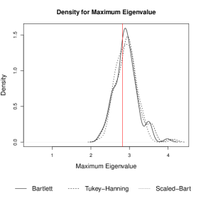
(a) $n=10^{3}$

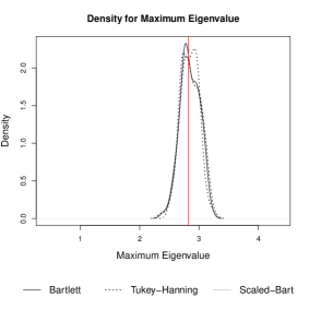
(b) $n=10^{4}$

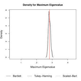
(c) $n=10^{5}$

Figure 6: Kernel density of the maximum eigenvalue for the three MSVEs over 100 replications and increasing Monte Carlo sample sizes for Setting 1. The vertical line indicates the true eigenvalue of 2.683 calculated using (3.2).

4 Discussion

Estimation of the asymptotic covariance matrix in the CLT as in (1.3) has received little attention in the MCMC literature thus far. Due to the results of this paper, practitioners are now equipped with a class of strongly consistent multivariate spectral variance estimators of $\Sigma$.

However, multivariate spectral variance estimators are also encountered outside of the MCMC context. For example, they are often used for heteroscedastic and autocorrelation consistent (HAC) estimation of covariance matrices which, for example, arise in the study of generalized method of moments and autoregressive processes with heteroscedastic errors. See Andrews, (1991) for motivating examples. In the context of HAC estimation, De Jong, (2000) obtained conditions under which the class of MSVEs are strongly consistent. However, these conditions are restrictive in the context of MCMC. In particular, his Assumption 2 (De Jong,, 2000, page 264) will not be satisfied in many typical MCMC applications. Additionally, we require weaker mixing conditions on the underlying stochastic process. That is, although Markov chains are the primary focus for us, our results hold for much more general stochastic processes as we explain below.

Our main assumption on the underlying stochastic process are the SIPs as stated in (2.3) and (2.4). The existence of an SIP has attracted much research interest. Consider the univariate case. For independent and identically distributed (i.i.d) processes, the first result of this kind is due to Strassen, (1964) who showed $\psi(n)=\sqrt{n\log\log n}$. Komlós et al., (1975) found that if $\text{E}_{F}|g|^{2+\delta}<\infty$, then $\psi(n)=n^{1/2-\lambda}$ for $\lambda>0$ (often called the KMT bound). Komlós et al., (1975) also showed that if $g$ has all moments in a neighborhood of 0, then $\psi(n)=\log n$. The results of Komlós et al., (1975) are the strongest to date in the i.i.d setting. The main reference for a univariate strong invariance principle for dependent sequences is Philipp and Stout, (1975) who prove bounds similar to that of Komlós et al., (1975) for a variety of weakly dependent processes including $\phi$-mixing, regenerative and strongly mixing processes. Also, see Wu, (2007) for a univariate strong invariance principle for certain classes of dependent processes.

Many of the univariate SIPs have been extended to the multivariate setting. For independent processes, Berkes and Philipp, (1979), Einmahl, (1989), and Zaitsev, (1998) extend the results of Komlós et al., (1975). For correlated processes, Eberlein, (1986) showed the existence of a strong invariance principle for Martingale sequences and Horvath, (1984) proved the KMT bound for multivariate extended renewal processes. For $\phi$-mixing, strongly mixing, and absolutely regular processes, Kuelbs and Philipp, (1980) and Dehling and Philipp, (1982) extended the Philipp and Stout, (1975) results to the multivariate case.

5 Acknowledgment

The authors thank Tiefeng Jiang and Gongjun Xu for helpful discussions.

Appendix A Strong Consistency of MSVE

Before we begin the proof of Theorem 1 we note some useful properties of Brownian motion and lag windows which will be used often throughout the proof.

A.1 Brownian Motion

Recall that $\{B(t)\}_{t\geq 0}$ denotes a $p$-dimensional standard Brownian motion and that $B^{(i)}$ denotes the $i$th component of $B(t)$.

Lemma 2 (Csörgő and Révész, (1981)).

Suppose Condition 2 holds, then for all $\epsilon>0$ and for almost all sample paths, there exists $n_{0}(\epsilon)$ such that for all $n\geq n_{0}$ and all $i=1,\dots,p$

$$\sup_{0\leq t\leq n-b_{n}}\sup_{0\leq s\leq b_{n}}\left|B^{(i)}(t+s)-B^{(i)}(t)\right|<(1+\epsilon)\left(2b_{n}\left(\log{\dfrac{n}{b_{n}}}+\log{\log n}\right)\right)^{1/2},$$

$$\sup_{0\leq s\leq b_{n}}\left|B^{(i)}(n)-B^{(i)}(n-s)\right|<(1+\epsilon)\left(2b_{n}\left(\log{\dfrac{n}{b_{n}}}+\log{\log n}\right)\right)^{1/2}\text{, and }$$

$$\left|B^{(i)}(n)\right|<(1+\epsilon)\sqrt{2n\log\log n}.$$

Let $L$ be a lower triangular matrix and set $\Sigma=LL^{T}$. Define $C(t):=LB(t)$ and if $C^{(i)}(t)$ is the $i$th component of $C(t)$, define

$$\bar{C}^{(i)}_{l}(k):=\dfrac{1}{k}\left(C^{(i)}(l+k)-C^{(i)}(l)\right)\text{ and }\bar{C}^{(i)}_{n}:=\dfrac{1}{n}C^{(i)}(n)\;.$$

Since $C^{(i)}(t)\sim N(0,t\Sigma_{ii})$, where $\Sigma_{ii}$ is the $i$th diagonal of $\Sigma$, $C^{(i)}/\sqrt{\Sigma_{ii}}$ is a 1-dimensional standard Brownian motion. As a consequence, we have the following corollaries of Lemma 2.

Corollary 1.

Suppose Condition 2 holds, then for all $\epsilon>0$ and for almost all sample paths there exists $n_{0}(\epsilon)$ such that for all $n\geq n_{0}$ and all $i=1,\dots,p$

$$\left|C^{(i)}(n)\right|<(1+\epsilon)(2n\Sigma_{ii}\log{\log n})^{1/2},$$ (A.1)

where $\Sigma_{ii}$ is the $i$th diagonal entry of $\Sigma$.

Corollary 2.

Suppose Condition 2 holds, then for all $\epsilon>0$ and for almost all sample paths, there exists $n_{0}(\epsilon)$ such that for all $n\geq n_{0}$ and all $i=1,\dots,p$

$$\left|\bar{C}^{(i)}_{l}(k)\right|\leq\dfrac{1}{k}\sup_{0\leq l\leq n-b_{n}}\sup_{0\leq s\leq b_{n}}\left|C^{(i)}(l+s)-C^{(i)}(l)\right|<\dfrac{1}{k}2(1+\epsilon)(b_{n}\Sigma_{ii}\log{n})^{1/2},$$ (A.2)

where $\Sigma_{ii}$ is the $i$th diagonal entry of $\Sigma$.

A.2 Basic Properties of Lag Windows

Recall that the lag window $w_{n}(\cdot)$ is such that it satisfies Condition 1. We will require the following results about the lag window $w_{n}(\cdot)$.

Lemma 3 (Damerdji, (1991)).

Under Condition 1,

1. $\Delta_{1}w_{n}(s)=\displaystyle\sum_{k=s}^{b_{n}}\Delta_{2}w_{n}(k)$,

2. $\displaystyle\sum_{k=s+1}^{b_{n}}\Delta_{1}w_{n}(k)=w_{n}(s)$, and

3. $\displaystyle\sum_{k=1}^{b_{n}}\Delta_{1}w_{n}(k)=1$.

A.3 Proof of Theorem 1

Recall that

$$\widehat{\Sigma}_{w,n}=\dfrac{1}{n}\displaystyle\sum_{l=0}^{n-b_{n}}\sum_{k=1}^{b_{n}}k^{2}\Delta_{2}w_{n}(k)[\bar{Y}_{l}(k)-\bar{Y}_{n}][\bar{Y}_{l}(k)-\bar{Y}_{n}]^{T}\,.$$ (A.3)

For $t=1,2,\dots,n$, define $Z_{t}=Y_{t}-\bar{Y}_{n}$ and

$$d_{n} =\dfrac{1}{n}\left\{\sum_{t=1}^{b_{n}}\Delta_{1}w_{n}(t)\left(\sum_{l=1}^{t-1}Z_{l}Z_{l}^{T}+\sum_{l=n-b_{n}+t+1}^{n}Z_{l}Z_{l}^{T}\right)\right.$$

$$\quad\left.+\sum_{s=1}^{b_{n}-1}\left[\sum_{t=1}^{b_{n}-s}\Delta_{1}w_{n}(s+t)\left(\sum_{l=1}^{t-1}\left(Z_{l}Z_{l+s}^{T}+Z_{l+s}Z_{l}^{T}\right)+\sum_{l=n-b_{n}+t+1}^{n-s}\left(Z_{l}Z_{l+s}^{T}+Z_{l+s}Z_{l}^{T}\right)\right)\right]\right\}\;.$$ (A.4)

Notice that in (A.4) we use the convention that empty sums are zero.

Lemma 4.

Under Condition 1, $\widehat{\Sigma}_{w,n}=\widehat{\Sigma}_{S}-d_{n}$.

Proof.

For $i,j=1,\dots,p$, let $\widehat{\Sigma}_{w,ij}$ denote the $(i,j)$th entry of $\widehat{\Sigma}_{w,n}$. Then,

$$\widehat{\Sigma}_{w,ij} =\dfrac{1}{n}\displaystyle\sum_{l=0}^{n-b_{n}}\displaystyle\sum_{k=1}^{b_{n}}k^{2}\Delta_{2}w_{n}(k)\left[\bar{Y}^{(i)}_{l}(k)-\bar{Y}^{(i)}_{n}\right]\left[\bar{Y}^{(j)}_{l}(k)-\bar{Y}^{(j)}_{n}\right]$$

$$=\dfrac{1}{n}\displaystyle\sum_{l=0}^{n-b_{n}}\displaystyle\sum_{k=1}^{b_{n}}\Delta_{2}w_{n}(k)\left[\displaystyle\sum_{t=1}^{k}Y^{(i)}_{l+t}-k\bar{Y}^{(i)}_{n}\right]\left[\displaystyle\sum_{t=1}^{k}Y^{(j)}_{l+t}-k\bar{Y}^{(j)}_{n}\right]$$

$$=\dfrac{1}{n}\displaystyle\sum_{l=0}^{n-b_{n}}\displaystyle\sum_{k=1}^{b_{n}}\Delta_{2}w_{n}(k)\left[\displaystyle\sum_{t=1}^{k}Z^{(i)}_{l+t}\right]\left[\displaystyle\sum_{t=1}^{k}Z^{(j)}_{l+t}\right]$$

$$=\dfrac{1}{n}\displaystyle\sum_{l=0}^{n-b_{n}}\displaystyle\sum_{k=1}^{b_{n}}\Delta_{2}w_{n}(k)\left[\displaystyle\sum_{t=1}^{k}Z^{(i)}_{l+t}Z^{(j)}_{l+t}+\displaystyle\sum_{s=1}^{k-1}\displaystyle\sum_{t=1}^{k-s}Z^{(i)}_{l+t}Z^{(j)}_{l+t+s}+\displaystyle\sum_{s=1}^{k-1}\displaystyle\sum_{t=1}^{k-s}Z^{(j)}_{l+t}Z^{(i)}_{l+t+s}\right].$$ (A.5)

Notice that in (A.5), we use the convention that empty sums are zero. We will consider each term in (A.5) separately. For the first term, changing the order of summation and then using Lemma 3,

$$\dfrac{1}{n}\displaystyle\sum_{l=0}^{n-b_{n}}\displaystyle\sum_{k=1}^{b_{n}}\displaystyle\sum_{t=1}^{k}\Delta_{2}w_{n}(k)Z^{(i)}_{l+t}Z^{(j)}_{l+t}$$

$$=\dfrac{1}{n}\displaystyle\sum_{l=0}^{n-b_{n}}\displaystyle\sum_{t=1}^{b_{n}}\displaystyle\sum_{k=t}^{b_{n}}\Delta_{2}w_{n}(k)Z^{(i)}_{l+t}Z^{(j)}_{l+t}$$

$$=\dfrac{1}{n}\displaystyle\sum_{l=0}^{n-b_{n}}\displaystyle\sum_{t=1}^{b_{n}}\Delta_{1}w_{n}(t)Z^{(i)}_{l+t}Z^{(j)}_{l+t}$$

$$=\dfrac{1}{n}\displaystyle\sum_{t=1}^{b_{n}}\Delta_{1}w_{n}(t)\displaystyle\sum_{l=0}^{n-b_{n}}Z^{(i)}_{l+t}Z^{(j)}_{l+t}$$

$$=\displaystyle\sum_{t=1}^{b_{n}}\Delta_{1}w_{n}(t)\left[\gamma_{n,ij}(0)-\dfrac{1}{n}\left(Z^{(i)}_{1}Z^{(j)}_{1}+\dots+Z^{(i)}_{t-1}Z^{(j)}_{t-1}+Z^{(i)}_{n-b_{n}+t+1}Z^{(j)}_{n-b_{n}+t+1}+\dots+Z^{(i)}_{n}Z^{(j)}_{n}\right)\right]$$

$$=\gamma_{n,ij}(0)-\dfrac{1}{n}\displaystyle\sum_{t=1}^{b_{n}}\Delta_{1}w_{n}(t)\left(\displaystyle\sum_{l=1}^{t-1}Z^{(i)}_{l}Z^{(j)}_{l}+\displaystyle\sum_{l=n-b_{n}+t+1}^{n}Z^{(i)}_{l}Z^{(j)}_{l}\right)\quad\text{by Lemma \ref{lemma:lag.res}}.$$ (A.6)

For the second term in (A.5) we change the order of summation from $l,k,s,t$ to $l,s,k,t$ to $l,s,t,k$ to get

$$\frac{1}{n}\sum_{l=0}^{n-b_{n}}\sum_{k=1}^{b_{n}}\sum_{s=1}^{k-1}\sum_{t=1}^{k-s}\Delta_{2}w_{n}(k)Z^{(i)}_{l+t}Z^{(j)}_{l+t+s}$$

$$=\dfrac{1}{n}\displaystyle\sum_{l=0}^{n-b_{n}}\displaystyle\sum_{s=1}^{b_{n}-1}\displaystyle\sum_{k=s+1}^{b_{n}}\displaystyle\sum_{t=1}^{k-s}\Delta_{2}w_{n}(k)Z^{(i)}_{l+t}Z^{(j)}_{l+t+s}$$

$$=\dfrac{1}{n}\displaystyle\sum_{l=0}^{n-b_{n}}\displaystyle\sum_{s=1}^{b_{n}-1}\displaystyle\sum_{t=1}^{b_{n}-s}\displaystyle\sum_{k=t+s}^{b_{n}}\Delta_{2}w_{n}(k)Z^{(i)}_{l+t}Z^{(j)}_{l+t+s}$$

$$=\dfrac{1}{n}\displaystyle\sum_{l=0}^{n-b_{n}}\displaystyle\sum_{s=1}^{b_{n}-1}\displaystyle\sum_{t=1}^{b_{n}-s}\Delta_{1}w_{n}(s+t)Z^{(i)}_{l+t}Z^{(j)}_{l+t+s}\quad\quad\text{by Lemma \ref{lemma:lag.res}}$$

$$=\dfrac{1}{n}\displaystyle\sum_{s=1}^{b_{n}-1}\displaystyle\sum_{l=0}^{n-b_{n}}\displaystyle\sum_{t=1}^{b_{n}-s}\Delta_{1}w_{n}(s+t)Z^{(i)}_{l+t}Z^{(j)}_{l+t+s}$$

$$=\dfrac{1}{n}\displaystyle\sum_{s=1}^{b_{n}-1}\displaystyle\sum_{t=1}^{b_{n}-s}\displaystyle\sum_{l=0}^{n-b_{n}}\Delta_{1}w_{n}(s+t)Z^{(i)}_{l+t}Z^{(j)}_{l+t+s}$$

$$=\dfrac{1}{n}\displaystyle\sum_{s=1}^{b_{n}-1}\displaystyle\sum_{t=1}^{b_{n}-s}\Delta_{1}w_{n}(s+t)\displaystyle\sum_{l=0}^{n-b_{n}}Z^{(i)}_{l+t}Z^{(j)}_{l+t+s}$$

$$=\displaystyle\sum_{s=1}^{b_{n}-1}\displaystyle\sum_{t=1}^{b_{n}-s}\Delta_{1}w_{n}(s+t)\left[\gamma_{n,ij}(s)-\dfrac{1}{n}\displaystyle\sum_{l=1}^{t-1}Z^{(i)}_{l}Z^{(j)}_{l+s}-\dfrac{1}{n}\displaystyle\sum_{l=n-b_{n}+t+1}^{n-s}Z^{(i)}_{l}Z^{(j)}_{l+s}\right]$$

$$=\displaystyle\sum_{s=1}^{b_{n}-1}w_{n}(s)\gamma_{n,ij}(s)$$

$$\quad-\dfrac{1}{n}\displaystyle\sum_{s=1}^{b_{n}-1}\displaystyle\sum_{t=1}^{b_{n}-s}\Delta_{1}w_{n}(s+t)\left[\displaystyle\sum_{l=1}^{t-1}Z^{(i)}_{l}Z^{(j)}_{l+s}+\displaystyle\sum_{l=n-b_{n}+t+1}^{n-s}Z^{(i)}_{l}Z^{(j)}_{l+s}\right]\quad\text{by Lemma \ref{lemma:lag.res}}.$$ (A.7)

Repeating the same steps as in the second term we reduce the third term in (A.5) to

$$\dfrac{1}{n}\displaystyle\sum_{l=0}^{n-b_{n}}\displaystyle\sum_{k=1}^{b_{n}}\sum_{s=1}^{k-1}\displaystyle\sum_{t=1}^{k-s}\Delta_{2}w_{n}(k)Z^{(j)}_{l+t}Z^{(i)}_{l+t+s}$$

$$=\displaystyle\sum_{s=1}^{b_{n}-1}w_{n}(s)\gamma_{n,ji}(s)-\dfrac{1}{n}\displaystyle\sum_{s=1}^{b_{n}-1}\displaystyle\sum_{t=1}^{b_{n}-s}\Delta_{1}w_{n}(s+t)\left[\displaystyle\sum_{l=1}^{t-1}Z^{(j)}_{l}Z^{(i)}_{l+s}+\displaystyle\sum_{l=n-b_{n}+t+1}^{n-s}Z^{(j)}_{l}Z^{(i)}_{l+s}\right]$$

$$=\displaystyle\sum_{s=1}^{b_{n}-1}w_{n}(-s)\gamma_{n,ij}(-s)-\dfrac{1}{n}\displaystyle\sum_{s=1}^{b_{n}-1}\displaystyle\sum_{t=1}^{b_{n}-s}\Delta_{1}w_{n}(s+t)\left[\displaystyle\sum_{l=1}^{t-1}Z^{(j)}_{l}Z^{(i)}_{l+s}+\displaystyle\sum_{l=n-b_{n}+t+1}^{n-s}Z^{(j)}_{l}Z^{(i)}_{l+s}\right]\;.$$ (A.8)

Using (A.6), (A.7), and (A.8) in (A.5)

$$\widehat{\Sigma}_{w,ij}= \,\gamma_{n,ij}(0)+\displaystyle\sum_{s=1}^{b_{n}-1}w_{n}(s)\gamma_{n,ij}(s)+\displaystyle\sum_{s=-(b_{n}-1)}^{-1}w_{n}(s)\gamma_{n,ij}(s)$$

$$-\dfrac{1}{n}\displaystyle\sum_{t=1}^{b_{n}}\Delta_{1}w_{n}(t)\left(\displaystyle\sum_{l=1}^{t-1}Z^{(i)}_{l}Z^{(j)}_{l}+\displaystyle\sum_{l=n-b_{n}+t+1}^{n}Z^{(i)}_{l}Z^{(j)}_{l}\right)$$

$$-\dfrac{1}{n}\displaystyle\sum_{s=1}^{b_{n}-1}\displaystyle\sum_{t=1}^{b_{n}-s}\Delta_{1}w_{n}(s+t)\left[\displaystyle\sum_{l=1}^{t-1}(Z^{(i)}_{l}Z^{(j)}_{l+s}+Z^{(i)}_{l+s}Z^{(j)}_{l})+\displaystyle\sum_{l=n-b_{n}+t+1}^{n-s}(Z^{(i)}_{l}Z^{(j)}_{l+s}+Z^{(i)}_{l+s}Z^{(j)}_{l})\right]$$

$$= \displaystyle\sum_{s=-(b_{n}-1)}^{b_{n}-1}\gamma_{n,ij}(s)w_{n}(s)-d_{n,ij}$$

$$= \widehat{\Sigma}_{S,ij}-d_{n,ij}.$$

∎

Let $\widetilde{\gamma}_{n}(s)$, $\widetilde{\Sigma}_{S},\widetilde{\Sigma}_{w,n}$ and $\tilde{d}_{n}$ be the Brownian motion analogs of (2.1), (2.2), (A.3), and (A.4). Specifically, for $t=1,\dots,n$, define Brownian motion increments $U_{t}=B(t)-B(t-1)$, so that $U_{1},\dots,U_{n}$ are $\overset{iid}{\sim}$ N${}_{p}(0,I_{p}$) where $I_{p}$ is the $p\times p$ identity matrix. For $l=0,\dots,n-b_{n}$ and $k=1,\dots,b_{n}$ define $\bar{B}_{l}(k)=k^{-1}(B(l+k)-B(l))$, $\bar{B}_{n}=n^{-1}B(n)$, and $T_{t}=U_{t}-\bar{B}_{n}$. Then

$$\widetilde{\gamma}_{n}(s)=\dfrac{1}{n}\displaystyle\sum_{t\in I_{s}}(U_{t}-\bar{B}_{n})(U_{t+s}-\bar{B}_{n})^{T}=\dfrac{1}{n}\displaystyle\sum_{t\in I_{s}}T_{t}T_{t+s}^{T},$$ (A.9)

$$\widetilde{\Sigma}_{S}=\displaystyle\sum_{s=-(b_{n}-1)}^{b_{n}-1}w_{n}(s)\widetilde{\gamma}_{n}(s),$$ (A.10)

$$\widetilde{\Sigma}_{w,n}=\dfrac{1}{n}\displaystyle\sum_{l=0}^{n-b_{n}}\sum_{k=1}^{b_{n}}k^{2}\Delta_{2}w_{n}(k)[\bar{B}_{l}(k)-\bar{B}_{n}][\bar{B}_{l}(k)-\bar{B}_{n}]^{T},$$ (A.11)

$$\tilde{d}_{n}=\dfrac{1}{n}\left\{\displaystyle\sum_{t=1}^{b_{n}}\Delta_{1}w_{n}(t)\left(\displaystyle\sum_{l=1}^{t-1}T_{l}T_{l}^{T}+\displaystyle\sum_{l=n-b_{n}+t+1}^{n}T_{l}T_{l}^{T}\right)\right.$$

$$\quad+\left.\displaystyle\sum_{s=1}^{b_{n}-1}\left[\displaystyle\sum_{t=1}^{b_{n}-s}\Delta_{1}w_{n}(s+t)\left(\displaystyle\sum_{l=1}^{t-1}(T_{l}T_{l+s}^{T}+T_{l+s}T_{l}^{T})+\sum_{l=n-b_{n}+t+1}^{n-s}(T_{l}T_{l+s}^{T}+T_{l+s}T_{l}^{T})\right)\right]\right\}.$$ (A.12)

Notice that in (A.12) we use the convention that empty sums are zero. Our goal is to show that $\widetilde{\Sigma}_{w,n}\to I_{p}$ as $n\to\infty$ with probability 1 in the following way. In Lemma 5 we show that $\widetilde{\Sigma}_{w,n}=\widetilde{\Sigma}_{S}-\tilde{d}_{n}$ and in Lemma 7 we show that the end term $\tilde{d}_{n}\to 0$ as $n\to\infty$ with probability 1. Lemma 12 shows that $\widetilde{\Sigma}_{S}\to I_{p}$ as $n\to\infty$ with probability 1, and hence $\widetilde{\Sigma}_{w,n}\to I_{p}$ as $n\to\infty$ with probability 1.

Lemma 5.

Under Condition 1, $\widetilde{\Sigma}_{w,n}=\widetilde{\Sigma}_{S}-\tilde{d}_{n}$.

Proof.

For $i,j=1,\dots,p$, let $\widetilde{\Sigma}_{w,ij}$ denote the $(i,j)$th entry of $\widetilde{\Sigma}_{w,n}$. Then,

$$\widetilde{\Sigma}_{w,ij} =\dfrac{1}{n}\displaystyle\sum_{l=0}^{n-b_{n}}\displaystyle\sum_{k=1}^{b_{n}}k^{2}\Delta_{2}w_{n}(k)\left[\bar{B}^{(i)}_{l}(k)-\bar{B}^{(i)}_{n}\right]\left[\bar{B}^{(j)}_{l}(k)-\bar{B}^{(j)}_{n}\right]$$

$$=\dfrac{1}{n}\displaystyle\sum_{l=0}^{n-b_{n}}\displaystyle\sum_{k=1}^{b_{n}}\Delta_{2}w_{n}(k)\left[B^{(i)}(k+l)-B^{(i)}(l)-k\bar{B}^{(i)}_{n}\right]\left[B^{(j)}(k+l)-B^{(j)}(l)-k\bar{B}^{(j)}_{n}\right]$$

$$=\dfrac{1}{n}\displaystyle\sum_{l=0}^{n-b_{n}}\displaystyle\sum_{k=1}^{b_{n}}\Delta_{2}w_{n}(k)\left[\displaystyle\sum_{t=1}^{k}U^{(i)}_{t+l}-k\bar{B}^{(i)}_{n}\right]\left[\displaystyle\sum_{t=1}^{k}U^{(j)}_{t+l}-k\bar{B}^{(j)}_{n}\right]$$

$$=\dfrac{1}{n}\displaystyle\sum_{l=0}^{n-b_{n}}\displaystyle\sum_{k=1}^{b_{n}}\Delta_{2}w_{n}(k)\left[\displaystyle\sum_{t=1}^{k}T^{(i)}_{t+l}\right]\left[\displaystyle\sum_{t=1}^{k}T^{(j)}_{t+l}\right]$$

$$=\dfrac{1}{n}\displaystyle\sum_{l=0}^{n-b_{n}}\displaystyle\sum_{k=1}^{b_{n}}\Delta_{2}w_{n}(k)\left[\displaystyle\sum_{t=1}^{k}T^{(i)}_{l+t}T^{(j)}_{l+t}+\displaystyle\sum_{s=1}^{k-1}\displaystyle\sum_{t=1}^{k-s}T^{(i)}_{l+t}T^{(j)}_{l+t+s}+\displaystyle\sum_{s=1}^{k-1}\displaystyle\sum_{t=1}^{k-s}T^{(j)}_{l+t}T^{(i)}_{l+t+s}\right].$$ (A.13)

In (A.13), we continue to use convention that empty sums are zero. We will look at each of the terms in (A.13) separately. For the first term, changing the order of summation and then using Lemma 3,

$$\dfrac{1}{n}\displaystyle\sum_{l=0}^{n-b_{n}}\displaystyle\sum_{k=1}^{b_{n}}\displaystyle\sum_{t=1}^{k}\Delta_{2}w_{n}(k)T^{(i)}_{l+t}T^{(j)}_{l+t}$$

$$=\dfrac{1}{n}\displaystyle\sum_{l=0}^{n-b_{n}}\displaystyle\sum_{t=1}^{b_{n}}\displaystyle\sum_{k=t}^{b_{n}}\Delta_{2}w_{n}(k)T^{(i)}_{l+t}T^{(j)}_{l+t}$$

$$=\dfrac{1}{n}\displaystyle\sum_{l=0}^{n-b_{n}}\displaystyle\sum_{t=1}^{b_{n}}T^{(i)}_{l+t}T^{(j)}_{l+t}\Delta_{1}w_{n}(t)$$

$$=\dfrac{1}{n}\displaystyle\sum_{t=1}^{b_{n}}\Delta_{1}w_{n}(t)\displaystyle\sum_{l=0}^{n-b_{n}}T^{(i)}_{l+t}T^{(j)}_{l+t}$$

$$=\widetilde{\gamma}_{n,ij}(0)-\dfrac{1}{n}\displaystyle\sum_{t=1}^{b_{n}}\Delta_{1}w_{n}(t)\left(\displaystyle\sum_{l=1}^{t-1}T^{(i)}_{l}T^{(j)}_{l}+\displaystyle\sum_{l=n-b_{n}+t+1}^{n}T^{(i)}_{l}T^{(j)}_{l}\right).$$ (A.14)

For the second term in (A.13) we change the order of summation from $l,k,s,t$ to $l,s,k,t$ then to $l,s,t,k$ and use Lemma 3 to get

$$\frac{1}{n}\sum_{l=0}^{n-b_{n}}\sum_{k=1}^{b_{n}}\sum_{s=1}^{k-1}\sum_{t=1}^{k-s}\Delta_{2}w_{n}(k)T^{(i)}_{l+t}T^{(j)}_{l+t+s}$$

$$=\dfrac{1}{n}\displaystyle\sum_{l=0}^{n-b_{n}}\displaystyle\sum_{s=1}^{b_{n}-1}\displaystyle\sum_{k=s+1}^{b_{n}}\displaystyle\sum_{t=1}^{k-s}\Delta_{2}w_{n}(k)T^{(i)}_{l+t}T^{(j)}_{l+t+s}$$

$$=\dfrac{1}{n}\displaystyle\sum_{l=0}^{n-b_{n}}\displaystyle\sum_{s=1}^{b_{n}-1}\displaystyle\sum_{t=1}^{b_{n}-s}\displaystyle\sum_{k=t+s}^{b_{n}}\Delta_{2}w_{n}(k)T^{(i)}_{l+t}T^{(j)}_{l+t+s}$$

$$=\dfrac{1}{n}\displaystyle\sum_{l=0}^{n-b_{n}}\displaystyle\sum_{s=1}^{b_{n}-1}\displaystyle\sum_{t=1}^{b_{n}-s}\Delta_{1}w_{n}(s+t)T^{(i)}_{l+t}T^{(j)}_{l+t+s}$$

$$=\dfrac{1}{n}\displaystyle\sum_{s=1}^{b_{n}-1}\displaystyle\sum_{l=0}^{n-b_{n}}\displaystyle\sum_{t=1}^{b_{n}-s}\Delta_{1}w_{n}(s+t)T^{(i)}_{l+t}T^{(j)}_{l+t+s}$$

$$=\dfrac{1}{n}\displaystyle\sum_{s=1}^{b_{n}-1}\displaystyle\sum_{t=1}^{b_{n}-s}\displaystyle\sum_{l=0}^{n-b_{n}}\Delta_{1}w_{n}(s+t)T^{(i)}_{l+t}T^{(j)}_{l+t+s}$$

$$=\dfrac{1}{n}\displaystyle\sum_{s=1}^{b_{n}-1}\displaystyle\sum_{t=1}^{b_{n}-s}\Delta_{1}w_{n}(s+t)\displaystyle\sum_{l=0}^{n-b_{n}}T^{(i)}_{l+t}T^{(j)}_{l+t+s}$$

$$=\dfrac{1}{n}\displaystyle\sum_{s=1}^{b_{n}-1}\displaystyle\sum_{t=1}^{b_{n}-s}\Delta_{1}w_{n}(s+t)\displaystyle\sum_{l=t}^{n-b_{n}+t}T^{(i)}_{l}T^{(j)}_{l+s}$$

$$=\displaystyle\sum_{s=1}^{b_{n}-1}\displaystyle\sum_{t=1}^{b_{n}-s}\Delta_{1}w_{n}(s+t)\left[\tilde{\gamma}_{n,ij}(s)-\dfrac{1}{n}\displaystyle\sum_{l=1}^{t-1}T^{(i)}_{l}T^{(j)}_{l+s}-\dfrac{1}{n}\displaystyle\sum_{l=n-b_{n}+t+1}^{n-s}T^{(i)}_{l}T^{(j)}_{l+s}\right]$$

$$=\displaystyle\sum_{s=1}^{b_{n}-1}w_{n}(s)\tilde{\gamma}_{n,ij}(s)-\dfrac{1}{n}\displaystyle\sum_{s=1}^{b_{n}-1}\displaystyle\sum_{t=1}^{b_{n}-s}\Delta_{1}w_{n}(s+t)\left[\displaystyle\sum_{l=1}^{t-1}T^{(i)}_{l}T^{(j)}_{l+s}+\displaystyle\sum_{l=n-b_{n}+t+1}^{n-s}T^{(i)}_{l}T^{(j)}_{l+s}\right].$$ (A.15)

Repeating the same steps as in the second term we reduce the third term in (A.13) to

$$\dfrac{1}{n}\displaystyle\sum_{l=0}^{n-b_{n}}\displaystyle\sum_{k=1}^{b_{n}}\displaystyle\sum_{s=1}^{k-1}\displaystyle\sum_{t=1}^{k-s}\Delta_{2}w_{n}(k)T^{(j)}_{l+t}T^{(i)}_{l+t+s}$$

$$=\displaystyle\sum_{s=1}^{b_{n}-1}w_{n}(s)\tilde{\gamma}_{n,ji}(s)-\dfrac{1}{n}\displaystyle\sum_{s=1}^{b_{n}-1}\displaystyle\sum_{t=1}^{b_{n}-s}\Delta_{1}w_{n}(s+t)\left[\displaystyle\sum_{l=1}^{t-1}T^{(j)}_{l}T^{(i)}_{l+s}+\displaystyle\sum_{l=n-b_{n}+t+1}^{n-s}T^{(j)}_{l}T^{(i)}_{l+s}\right]$$

$$=\displaystyle\sum_{s=1}^{b_{n}-1}w_{n}(-s)\tilde{\gamma}_{n,ij}(-s)-\dfrac{1}{n}\displaystyle\sum_{s=1}^{b_{n}-1}\displaystyle\sum_{t=1}^{b_{n}-s}\Delta_{1}w_{n}(s+t)\left[\displaystyle\sum_{l=1}^{t-1}T^{(j)}_{l}T^{(i)}_{l+s}+\displaystyle\sum_{l=n-b_{n}+t+1}^{n-s}T^{(j)}_{l}T^{(i)}_{l+s}\right].$$ (A.16)

Using (A.14), (A.15), and (A.16) in (A.13), we get

$$\widetilde{\Sigma}_{w,ij}= \,\tilde{\gamma}_{n,ij}(0)+\displaystyle\sum_{s=1}^{b_{n}-1}w_{n}(s)\tilde{\gamma}_{n,ij}(s)+\displaystyle\sum_{s=-(b_{n}-1)}^{-1}w_{n}(s)\tilde{\gamma}_{n,ij}(s)$$

$$-\dfrac{1}{n}\displaystyle\sum_{t=1}^{b_{n}}\Delta_{1}w_{n}(t)\left(\displaystyle\sum_{l=1}^{t-1}T^{(i)}_{l}T^{(j)}_{l}+\displaystyle\sum_{l=n-b_{n}+t+1}^{n}T^{(i)}_{l}T^{(j)}_{l}\right)$$

$$-\dfrac{1}{n}\displaystyle\sum_{s=1}^{b_{n}-1}\displaystyle\sum_{t=1}^{b_{n}-s}\Delta_{1}w_{n}(s+t)\left[\displaystyle\sum_{l=1}^{t-1}(T^{(i)}_{l}T^{(j)}_{l+s}+T^{(i)}_{l+s}T^{(j)}_{l})+\displaystyle\sum_{l=n-b_{n}+t+1}^{n-s}(T^{(i)}_{l}T^{(j)}_{l+s}+T^{(i)}_{l+s}T^{(j)}_{l})\right]$$

$$= \displaystyle\sum_{s=-(b_{n}-1)}^{b_{n}-1}\tilde{\gamma}_{n,ij}(s)w_{n}(s)-\tilde{d}_{n,ij}$$

$$= \widetilde{\Sigma}_{S,ij}-\tilde{d}_{n,ij}.$$

∎

Next, we show that as $n\to\infty$, $\tilde{d}_{n}\to 0$ with probability 1 implying $\widetilde{\Sigma}_{w,n}-\widetilde{\Sigma}_{S}\to 0$ with probability 1 as $n\to\infty$. To do so we require a strong invariance principle for independent and identically distributed random variables.

Theorem 4 (Komlós et al., (1975)).

Let $B(n)$ be a 1-dimensional standard Brownian motion. If $X_{1},X_{2},X_{3}\dots$ are independent and identically distributed univariate random variables with mean $\mu$ and standard deviation $\sigma$, such that $\text{E}\left[e^{|tX_{1}|}\right]<\infty$ in a neighborhood of $t=0$, then as $n\to\infty$

$$\sum_{i=1}^{n}X_{i}-n\mu-\sigma B(n)=O(\log n)\;.$$

We begin with a technical lemma that will be used in a couple of places in the rest of the proof.

Lemma 6.

Let Conditions 1 and 2 hold. If, as $n\to\infty$, $b_{n}n^{-1}\sum_{k=1}^{b_{n}}k|\Delta_{1}w_{n}(k)|\to 0$, then

$$\dfrac{b_{n}}{n}\left(\sum_{t=1}^{b_{n}}|\Delta_{1}w_{n}(t)|+2\displaystyle\sum_{s=1}^{b_{n}-1}\displaystyle\sum_{t=1}^{b_{n}-s}|\Delta_{1}w_{n}(s+t)|\right)\to 0\;.$$

Proof.

$$\dfrac{b_{n}}{n}\left(\sum_{t=1}^{b_{n}}|\Delta_{1}w_{n}(t)|+2\displaystyle\sum_{s=1}^{b_{n}-1}\displaystyle\sum_{t=1}^{b_{n}-s}|\Delta_{1}w_{n}(s+t)|\right)$$

$$=\dfrac{b_{n}}{n}\left(\sum_{t=1}^{b_{n}}|\Delta_{1}w_{n}(t)|+2\displaystyle\sum_{s=1}^{b_{n}-1}\displaystyle\sum_{k=s+1}^{b_{n}}|\Delta_{1}w_{n}(k)|\right)$$

$$=\dfrac{b_{n}}{n}\left(\sum_{t=1}^{b_{n}}|\Delta_{1}w_{n}(t)|+2\displaystyle\sum_{k=2}^{b_{n}}\displaystyle\sum_{s=1}^{k-1}|\Delta_{1}w_{n}(k)|\right)$$

$$=\dfrac{b_{n}}{n}\left(\sum_{t=1}^{b_{n}}|\Delta_{1}w_{n}(t)|+2\displaystyle\sum_{k=2}^{b_{n}}(k-1)|\Delta_{1}w_{n}(k)|\right)$$

$$=\dfrac{b_{n}}{n}\left(\sum_{t=1}^{b_{n}}|\Delta_{1}w_{n}(t)|+2\displaystyle\sum_{k=1}^{b_{n}}(k-1)|\Delta_{1}w_{n}(k)|\right)$$

$$\leq\dfrac{b_{n}}{n}\left(2\displaystyle\sum_{k=1}^{b_{n}}k|\Delta_{1}w_{n}(k)|\right)$$

$$\to 0\text{ by assumption}.$$

∎

Lemma 7.

Let Conditions 1 and 2 hold and let $n>2b_{n}$. If $b_{n}n^{-1}\sum_{k=1}^{b_{n}}k|\Delta_{1}w_{n}(k)|\to 0$ and $b_{n}^{-1}\log n=O(1)$ as $n\to\infty$, then $\tilde{d}_{n}\to 0$ with probability 1 as $n\to\infty$.

Proof.

For $i,j=1,\dots,p$, we will show that as $n\to\infty$ with probability 1, $\tilde{d}_{n,ij}\to 0$. Recall

$$\tilde{d}_{n,ij} =\dfrac{1}{n}\displaystyle\sum_{t=1}^{b_{n}}\Delta_{1}w_{n}(t)\left(\displaystyle\sum_{l=1}^{t-1}T^{(i)}_{l}T^{(j)}_{l}+\displaystyle\sum_{l=n-b_{n}+t+1}^{n}T^{(i)}_{l}T^{(j)}_{l}\right)$$

$$\quad+\dfrac{1}{n}\displaystyle\sum_{s=1}^{b_{n}-1}\displaystyle\sum_{t=1}^{b_{n}-s}\Delta_{1}w_{n}(s+t)\left[\displaystyle\sum_{l=1}^{t-1}(T^{(i)}_{l}T^{(j)}_{l+s}+T^{(i)}_{l+s}T^{(j)}_{l})+\displaystyle\sum_{l=n-b_{n}+t+1}^{n-s}(T^{(i)}_{l}T^{(j)}_{l+s}+T^{(i)}_{l+s}T^{(j)}_{l})\right]$$

$$|\tilde{d}_{n,ij}| \leq\dfrac{1}{n}\displaystyle\sum_{t=1}^{b_{n}}|\Delta_{1}w_{n}(t)|\left(\displaystyle\sum_{l=1}^{t-1}\left|T^{(i)}_{l}T^{(j)}_{l}\right|+\displaystyle\sum_{l=n-b_{n}+t+1}^{n}\left|T^{(i)}_{l}T^{(j)}_{l}\right|\right)$$

$$\quad+\dfrac{1}{n}\displaystyle\sum_{s=1}^{b_{n}-1}\displaystyle\sum_{t=1}^{b_{n}-s}|\Delta_{1}w_{n}(s+t)|\,\,\times$$

$$\quad\times\left[\displaystyle\sum_{l=1}^{t-1}\left(\left|T^{(i)}_{l}T^{(j)}_{l+s}\right|+\left|T^{(i)}_{l+s}T^{(j)}_{l}\right|\right)+\displaystyle\sum_{l=n-b_{n}+t+1}^{n-s}\left(\left|T^{(i)}_{l}T^{(j)}_{l+s}\right|+\left|T^{(i)}_{l+s}T^{(j)}_{l}\right|\right)\right],$$ (A.17)

where we use the convention that empty sums are zero. Using the inequality $|ab|\leq(a^{2}+b^{2})/2$ in the first and second terms in (A.17), we have for $t=1,\dots,b_{n}$

$$\sum_{l=1}^{t-1}\left|T^{(i)}_{l}T^{(j)}_{l}\right|\leq\dfrac{1}{2}\displaystyle\sum_{l=1}^{t-1}\left(T^{(i)2}_{l}+T^{(j)2}_{l}\right)\leq\dfrac{1}{2}\displaystyle\sum_{l=1}^{2b_{n}}T^{(i)2}_{l}+\dfrac{1}{2}\displaystyle\sum_{l=1}^{2b_{n}}T^{(j)2}_{l}$$

$$\sum_{l=n-b_{n}+t+1}^{n}\left|T^{(i)}_{l}T^{(j)}_{l}\right|\leq\dfrac{1}{2}\displaystyle\sum_{l=n-b_{n}+t+1}^{n}\left(T^{(i)2}_{l}+T^{(j)2}_{l}\right)\leq\dfrac{1}{2}\displaystyle\sum_{l=n-2b_{n}+1}^{n}T^{(i)2}_{l}+\dfrac{1}{2}\displaystyle\sum_{l=n-2b_{n}+1}^{n}T^{(j)2}_{l}.$$

Similarly, for the third and fourth terms in (A.17), for $t=1,\dots b_{n}-1$ and $s=1,\dots,b_{n}-1$

$$\displaystyle\sum_{l=1}^{t-1}\left|T^{(i)}_{l}T^{(j)}_{l+s}\right|+\displaystyle\sum_{l=1}^{t-1}\left|T^{(i)}_{l+s}T^{(j)}_{l}\right| \leq\dfrac{1}{2}\displaystyle\sum_{l=1}^{2b_{n}}T^{(i)2}_{l}+\dfrac{1}{2}\displaystyle\sum_{l=1}^{2b_{n}}T^{(j)2}_{l}+\dfrac{1}{2}\displaystyle\sum_{l=1}^{b_{n}}T^{(j)2}_{l+s}+\dfrac{1}{2}\displaystyle\sum_{l=1}^{b_{n}}T^{(i)2}_{l+s}$$

$$\leq\dfrac{1}{2}\displaystyle\sum_{l=1}^{2b_{n}}T^{(i)2}_{l}+\dfrac{1}{2}\displaystyle\sum_{l=1}^{2b_{n}}T^{(j)2}_{l}+\dfrac{1}{2}\displaystyle\sum_{l=1}^{2b_{n}}T^{(j)2}_{l}+\dfrac{1}{2}\displaystyle\sum_{l=1}^{2b_{n}}T^{(i)2}_{l}$$

$$=\sum_{l=1}^{2b_{n}}T^{(i)2}_{l}+\displaystyle\sum_{l=1}^{2b_{n}}T^{(j)2}_{l}.$$

$$\sum_{l=n-b_{n}+t+1}^{n}\left|T^{(i)}_{l}T^{(j)}_{l+s}\right|+\sum_{l=n-b_{n}+t+1}^{n}\left|T^{(i)}_{l+s}T^{(j)}_{l}\right|$$

$$\leq\dfrac{1}{2}\displaystyle\sum_{l=n-2b_{n}+1}^{n}(T^{(i)2}_{l}+T^{(j)2}_{l})+\dfrac{1}{2}\displaystyle\sum_{l=n-b_{n}+1}^{n}(T^{(j)2}_{l+s}+T^{(i)2}_{l+s})$$

$$\leq\dfrac{1}{2}\displaystyle\sum_{l=n-2b_{n}+1}^{n}(T^{(i)2}_{l}+T^{(j)2}_{l})+\dfrac{1}{2}\displaystyle\sum_{l=n-2b_{n}+1}^{n}(T^{(j)2}_{l}+T^{(i)2}_{l})$$

$$=\displaystyle\sum_{l=n-2b_{n}+1}^{n}T^{(i)2}_{l}+\displaystyle\sum_{l=n-2b_{n}+1}^{n}T^{(j)2}_{l}.$$

Combining the above results in (A.17) we get,

$$|\tilde{d}_{n,ij}| \leq\dfrac{1}{n}\left(\dfrac{1}{2}\displaystyle\sum_{l=1}^{2b_{n}}T^{(i)2}_{l}+\dfrac{1}{2}\displaystyle\sum_{l=1}^{2b_{n}}T^{(j)2}_{l}+\dfrac{1}{2}\displaystyle\sum_{l=n-2b_{n}+1}^{n}T^{(i)2}_{l}+\dfrac{1}{2}\displaystyle\sum_{l=n-2b_{n}+1}^{n}T^{(j)2}_{l}\right)\displaystyle\sum_{t=1}^{b_{n}}|\Delta_{1}w_{n}(t)|$$

$$+\dfrac{1}{n}\displaystyle\sum_{s=1}^{b_{n}-1}\left[\left(\displaystyle\sum_{l=1}^{2b_{n}}T^{(i)2}_{l}+\displaystyle\sum_{l=1}^{2b_{n}}T^{(j)2}_{l}+\displaystyle\sum_{l=n-2b_{n}+1}^{n}T^{(i)2}_{l}+\displaystyle\sum_{l=n-2b_{n}+1}^{n}T^{(j)2}_{l}\right)\displaystyle\sum_{t=1}^{b_{n}-s}|\Delta_{1}w_{n}(s+t)|\right]$$

$$=\dfrac{1}{b_{n}}\left(\dfrac{1}{2}\displaystyle\sum_{l=1}^{2b_{n}}T^{(i)2}_{l}+\dfrac{1}{2}\displaystyle\sum_{l=1}^{2b_{n}}T^{(j)2}_{l}+\dfrac{1}{2}\displaystyle\sum_{l=n-2b_{n}+1}^{n}T^{(i)2}_{l}+\dfrac{1}{2}\displaystyle\sum_{l=n-2b_{n}+1}^{n}T^{(j)2}_{l}\right)\times$$

$$\dfrac{b_{n}}{n}\left(\sum_{t=1}^{b_{n}}|\Delta_{1}w_{n}(t)|+2\displaystyle\sum_{s=1}^{b_{n}-1}\displaystyle\sum_{t=1}^{b_{n}-s}|\Delta_{1}w_{n}(s+t)|\right).$$ (A.18)

We will show that the first term in the product in (A.18) remains bounded with probability 1 as $n\to\infty$. Consider,

$$\dfrac{1}{2b_{n}}\displaystyle\sum_{l=1}^{2b_{n}}T_{l}^{(i)2} =\dfrac{1}{2b_{n}}\displaystyle\sum_{l=1}^{2b_{n}}\left(U_{l}^{(i)}-\bar{B}^{(i)}_{n}\right)^{2}$$

$$=\dfrac{1}{2b_{n}}\displaystyle\sum_{l=1}^{2b_{n}}U_{l}^{(i)2}-2\bar{B}^{(i)}_{n}\dfrac{1}{2b_{n}}\displaystyle\sum_{l=1}^{2b_{n}}U_{l}^{(i)}+\left(\bar{B}^{(i)}_{n}\right)^{2}$$

$$\leq\left|\dfrac{1}{2b_{n}}\displaystyle\sum_{l=1}^{2b_{n}}U_{l}^{(i)2}\right|+2\left|\bar{B}_{n}^{(i)}\right|\left|\dfrac{1}{2b_{n}}\displaystyle\sum_{l=1}^{2b_{n}}U_{l}^{(i)}\right|+\left|\bar{B}_{n}^{(i)}\right|^{2}$$

$$<\left|\dfrac{1}{2b_{n}}\displaystyle\sum_{l=1}^{2b_{n}}U_{l}^{(i)2}\right|+\left|\dfrac{1}{2b_{n}}\displaystyle\sum_{l=1}^{2b_{n}}U_{l}^{(i)}\right|\left(\dfrac{2}{n}(1+\epsilon)(2n\log\log n)^{1/2}\right)$$

$$\quad+\left(\dfrac{1}{n}(1+\epsilon)(2n\log\log n)^{1/2}\right)^{2}\quad\quad\text{by Lemma \ref{bn.diff.bound}}$$

$$<\left|\dfrac{1}{2b_{n}}\displaystyle\sum_{l=1}^{2b_{n}}U_{l}^{(i)2}\right|+\left|\dfrac{1}{2b_{n}}\displaystyle\sum_{l=1}^{2b_{n}}U_{l}^{(i)}\right|O((n^{-1}\log n)^{1/2})+O(n^{-1}\log n)\;.$$

Since $U_{l}^{(i)}$ are Brownian motion increments, $U^{(i)}_{l}\overset{iid}{\sim}N(0,1)$ and by the classical strong law of large numbers, the above remains bounded with probability 1. Similarly $(2b_{n})^{-1}\sum_{l=1}^{2b_{n}}T_{l}^{(j)2}$ remains bounded with probability 1 as $n\to\infty$. Next, consider $R_{n}=\sum_{l=1}^{n}U_{l}^{(i)2}$. Since $U_{l}^{(i)}\sim N(0,1)$, $R_{n}\sim\chi^{2}_{n}$. Thus $R_{n}$ has a moment generating function and an application of Theorem 4 implies there exists a finite random variable $C_{R}$ such that, for sufficiently large $n$,

$$\left|R_{n}-n-2B^{(i)}(n)\right|<C_{R}\log n\;.$$ (A.19)

Consider

$$\left|R_{n}-R_{n-2b_{n}}\right| =\Big{|}\left(R_{n}-n-2B^{(i)}(n)\right)-\left(R_{n-2b_{n}}-(n-2b_{n})-2B^{(i)}(n-2b_{n})\right)$$

$$\quad-(n-2b_{n})+n+2B^{(i)}(n)-2B^{(i)}(n-2b_{n})\Big{|}$$

$$\leq\left|\left(R_{n}-n-2B^{(i)}(n)\right)\right|+\left|\left(R_{n-2b_{n}}-(n-2b_{n})-2B^{(i)}(n-2b_{n})\right)\right|$$

$$\quad+\left|2b_{n}+2B^{(i)}(n)-2B^{(i)}(n-2b_{n})\right|$$

$$<C_{R}\log{n}+C_{R}\log{(n-b_{n})}+2b_{n}$$

$$\quad+2(1+\epsilon)\left(2(2b_{n})\left(\log{\dfrac{n}{2b_{n}}}+\log\log n\right)\right)^{1/2}\quad\text{by \eqref{eq:rn_kmt} and Lemma \ref{bn.diff.bound}}$$

$$<2C_{R}\log n+2b_{n}+4(1+\epsilon)(2b_{n}\log n)^{1/2}.$$ (A.20)

Finally,

$$\frac{1}{2b_{n}}\sum_{l=n-2b_{n}+1}^{n}T_{l}^{(i)2}$$

$$=\dfrac{1}{2b_{n}}\displaystyle\sum_{l=n-2b_{n}+1}^{n}\left(U_{l}^{(i)}-\bar{B}^{(i)}_{n}\right)^{2}$$

$$=\dfrac{1}{2b_{n}}\displaystyle\sum_{l=n-2b_{n}+1}^{n}U_{l}^{(i)2}-\dfrac{2\bar{B}^{(i)}_{n}}{2b_{n}}\displaystyle\sum_{l=n-2b_{n}+1}^{n}U_{l}^{(i)}+\left(\bar{B}^{(i)}_{n}\right)^{2}$$

$$=\dfrac{1}{2b_{n}}(R_{n}-R_{n-2b_{n}})-\dfrac{2}{n}B^{(i)}(n)\dfrac{1}{2b_{n}}\left(B^{(i)}(n)-B^{(i)}(n-2b_{n})\right)+\left(\dfrac{1}{n}B^{(i)}(n)\right)^{2}$$

$$<\dfrac{1}{2b_{n}}|R_{n}-R_{n-2b_{n}}|+\dfrac{2}{n}\left|B^{(i)}(n)\right|\dfrac{1}{2b_{n}}\left|B^{(i)}(n)-B^{(i)}(n-2b_{n})\right|+\left(\dfrac{1}{n}\left|B^{(i)}(n)\right|\right)^{2}$$

$$<\dfrac{1}{2b_{n}}\left(2C_{R}\log n+2b_{n}+4(1+\epsilon)(2b_{n}\log n)^{1/2}\right)$$

$$\quad+\dfrac{2}{n}(1+\epsilon)(2n\log\log n)^{1/2}\dfrac{1}{2b_{n}}(1+\epsilon)\left(2(2b_{n})\left(\log{\dfrac{n}{2b_{n}}}+\log\log n\right)\right)^{1/2}$$

$$\quad+\left(\dfrac{1}{n}(1+\epsilon)(2n\log\log n)^{1/2}\right)^{2}\quad\quad\text{by \eqref{eq:rn_diff} and Lemma \ref{bn.diff.bound}}$$

$$<C_{R}b_{n}^{-1}\log n+1+\dfrac{4(1+\epsilon)(2b_{n}\log n)^{1/2}}{2b_{n}}+\dfrac{1}{nb_{n}}(1+\epsilon)^{2}(2n\log n)^{1/2}(8b_{n}\log n)^{1/2}$$

$$\quad+\dfrac{(1+\epsilon)^{2}}{n}(2\log n)$$

$$<C_{R}b_{n}^{-1}\log n+1+2(1+\epsilon)(2b_{n}^{-1}\log n)^{1/2}+4(1+\epsilon)^{2}\left(\dfrac{\log n}{n}\right)^{1/2}\left(b_{n}^{-1}\log n\right)^{1/2}+2(1+\epsilon)^{2}\dfrac{\log n}{n}.$$

Since $b_{n}^{-1}\log n=O(1)$ as $n\to\infty$, the above term remains bounded with probability 1 as $n\to\infty$. Similarly, $(2b_{n})^{-1}\sum_{l=n-2b_{n}+1}^{n}T_{l}^{(j)2}$ remains bounded with probability 1 as $n\to\infty$. The second term in the product in (A.18) converges to 0 by Lemma 6 and hence $\tilde{d}_{n,ij}\to 0$ with probability 1 as $n\to\infty$. ∎

Recall that $h(X_{t})=Y_{t}^{2}$ for $t=1,2,3,\dots$, where the square is element-wise.

Lemma 8.

Let a strong invariance principle for $h$ hold as in (2.4). If Condition 2 holds, $b_{n}^{-1}\psi_{h}(n)\to 0$ and $b_{n}^{-1}\log n=O(1)$ as $n\to\infty$, then

$$\dfrac{1}{b_{n}}\displaystyle\sum_{k=1}^{b_{n}}h(X_{k})\text{ and }\dfrac{1}{b_{n}}\displaystyle\sum_{k=n-b_{n}+1}^{n}h(X_{k}),$$

stay bounded with probability 1 as $n\to\infty$.

Proof.

Equation (2.4) implies that $b_{n}^{-1}\sum_{k=1}^{b_{n}}h(X_{k})\to\text{E}_{F}h$ if $b_{n}^{-1}\psi_{h}(b_{n})\to 0$ as $n\to\infty$. Since by assumption $b_{n}^{-1}\psi_{h}(n)\to 0$ as $n\to\infty$ and $\psi_{h}$ is increasing, $b_{n}^{-1}\sum_{k=1}^{b_{n}}h(X_{k})$ remains bounded w.p. 1 as $n\to\infty$. Next, for all $\epsilon>0$ and sufficiently large $n(\epsilon)$,

$$\dfrac{1}{b_{n}}\left\|\displaystyle\sum_{k=n-b_{n}+1}^{n}h(X_{k})\right\|$$

$$= \dfrac{1}{b_{n}}\left\|\displaystyle\sum_{k=1}^{n}h(X_{k})-\displaystyle\sum_{k=1}^{n-b_{n}}h(X_{k})\right\|$$

$$= \dfrac{1}{b_{n}}\Bigg{\|}\displaystyle\sum_{k=1}^{n}h(X_{k})-n\text{E}_{F}h+(n-b_{n})\text{E}_{F}h+b_{n}\text{E}_{F}h-L_{h}B(n)+L_{h}B(n-b_{n})$$

$$+L_{h}(B(n)-B(n-b_{n}))-\displaystyle\sum_{k=1}^{n-b_{n}}h(X_{k})\Bigg{\|}$$

$$\leq \dfrac{1}{b_{n}}\left\|\displaystyle\sum_{k=1}^{n}h(X_{k})-n\text{E}_{F}h-L_{h}B(n)\right\|+\dfrac{1}{b_{n}}\left\|\displaystyle\sum_{k=1}^{n-b_{n}}h(X_{k})-(n-b_{n})\text{E}_{F}h-L_{h}B(n-b_{n})\right\|$$

$$+\dfrac{1}{b_{n}}\left\|L_{h}(B(n)-B(n-b_{n}))+b_{n}\text{E}_{F}h\right\|$$

$$< \dfrac{1}{b_{n}}D_{h}\psi_{h}(n)+\dfrac{1}{b_{n}}D_{h}\psi_{h}(n-b_{n})+\dfrac{1}{b_{n}}\left\|L_{h}(B(n)-B(n-b_{n}))\right\|+\left\|\text{E}_{F}h\right\|\quad\quad\text{by \eqref{eq:multi_sip_h}}$$

$$\leq \dfrac{1}{b_{n}}D_{h}\psi_{h}(n)+\dfrac{1}{b_{n}}D_{h}\psi_{h}(n-b_{n})+\dfrac{1}{b_{n}}\|L_{h}\|\left(\displaystyle\sum_{i=1}^{p}\left|B^{(i)}(n)-B^{(i)}(n-b_{n})\right|^{2}\right)^{1/2}+\|\text{E}_{F}h\|$$

$$\leq \dfrac{1}{b_{n}}D_{h}\psi_{h}(n)+\dfrac{1}{b_{n}}D_{h}\psi_{h}(n-b_{n})+\dfrac{1}{b_{n}}\|L_{h}\|\left(\displaystyle\sum_{i=1}^{p}\sup_{0\leq s\leq b_{n}}\left|B^{(i)}(n)-B^{(i)}(n-s)\right|^{2}\right)^{1/2}+\|\text{E}_{F}h\|$$

$$< \dfrac{2}{b_{n}}D_{h}\psi_{h}(n)+\dfrac{p^{1/2}}{b_{n}}\|L_{h}\|(1+\epsilon)\left(2b_{n}\left(\log{\dfrac{n}{b_{n}}}+\log{\log n}\right)\right)^{1/2}+\left\|\text{E}_{F}h\right\|\quad\quad\text{by Lemma \ref{bn.diff.bound}}$$

$$< \left\|\text{E}_{F}h\right\|+\dfrac{2}{b_{n}}D_{h}\psi_{h}(n)+O((b_{n}^{-1}\log n)^{1/2}).$$

Thus by the assumptions $b_{n}^{-1}\left\|\sum_{k=n-b_{n}+1}^{n}h(X_{k})\right\|$ stays bounded w.p. 1 as $n\to\infty$. ∎

Lemma 9.

Suppose the strong invariance principles (2.3) and (2.4) hold. In addition, suppose Conditions 1 and 2 hold and $n>2b_{n}$, $b_{n}n^{-1}\sum_{k=1}^{b_{n}}k|\Delta_{1}w_{n}(k)|\to 0$, $b_{n}^{-1}\psi(n)\to 0$, $b_{n}^{-1}\psi_{h}(n)\to 0$ as $n\to\infty$ and $b_{n}^{-1}\log n=O(1)$. Then, $d_{n}\to 0$ with probability 1 as $n\to\infty$.

Proof.

For $i,j=1,\dots,p$, let $d_{n,ij}$ denote the $(i,j)$th element of the matrix $d_{n}$. We can follow the same steps as in Lemma 7 to obtain

$$|d_{n,ij}| \leq\dfrac{1}{b_{n}}\left(\dfrac{1}{2}\displaystyle\sum_{l=1}^{2b_{n}}Z^{(i)2}_{l}+\dfrac{1}{2}\displaystyle\sum_{l=1}^{2b_{n}}Z^{(j)2}_{l}+\dfrac{1}{2}\displaystyle\sum_{l=n-2b_{n}+1}^{n}Z^{(i)2}_{l}+\dfrac{1}{2}\displaystyle\sum_{l=n-2b_{n}+1}^{n}Z^{(j)2}_{l}\right)\times$$

$$\dfrac{b_{n}}{n}\left(\sum_{t=1}^{b_{n}}|\Delta_{1}w_{n}(t)|+2\displaystyle\sum_{s=1}^{b_{n}-1}\displaystyle\sum_{t=1}^{b_{n}-s}|\Delta_{1}w_{n}(s+t)|\right).$$

The second term in the product converges to 0 by Lemma 6. It remains to show that the following remains bounded with probability 1 as $n\to\infty$,

$$\dfrac{1}{b_{n}}\left(\dfrac{1}{2}\displaystyle\sum_{l=1}^{2b_{n}}Z^{(i)2}_{l}+\dfrac{1}{2}\displaystyle\sum_{l=1}^{2b_{n}}Z^{(j)2}_{l}+\dfrac{1}{2}\displaystyle\sum_{l=n-2b_{n}+1}^{n}Z^{(i)2}_{l}+\dfrac{1}{2}\displaystyle\sum_{l=n-2b_{n}+1}^{n}Z^{(j)2}_{l}\right).$$

We have,

$$\dfrac{1}{2b_{n}}\displaystyle\sum_{l=1}^{2b_{n}}Z_{l}^{(i)2} =\dfrac{1}{2b_{n}}\displaystyle\sum_{l=1}^{2b_{n}}\left(Y_{l}^{(i)}-\bar{Y}^{(i)}_{n}\right)^{2}=\dfrac{1}{2b_{n}}\displaystyle\sum_{l=1}^{2b_{n}}Y_{l}^{(i)2}-2\bar{Y}^{(i)}_{2b_{n}}\bar{Y}^{(i)}_{n}+\left(\bar{Y}^{(i)}_{n}\right)^{2}.$$

By the strong invariance principle for $g$, $\bar{Y}_{n}^{(i)}\to 0$, $\bar{Y}_{2b_{n}}^{(i)}\to 0$, and $(\bar{Y}^{(i)}_{n})^{2}\to 0$ w.p. 1 as $n\to\infty$. By Lemma 8, $(2b_{n})^{-1}\sum_{l=1}^{2b_{n}}Y_{l}^{(i)2}$ remains bounded w.p. 1 as $n\to\infty$. Thus $(2b_{n})^{-1}\sum_{l=1}^{2b_{n}}Z_{l}^{(i)2}$ remains bounded w.p. 1 as $n\to\infty$. Similarly $(2b_{n})^{-1}\sum_{l=1}^{2b_{n}}Z_{l}^{(j)2}$ stay bounded w.p. 1 as $n\to\infty$. Now consider

$$\dfrac{1}{2b_{n}}\displaystyle\sum_{l=n-2b_{n}+1}^{n}Z_{l}^{(i)2} =\dfrac{1}{2b_{n}}\displaystyle\sum_{l=n-2b_{n}+1}^{n}\left(Y_{l}^{(i)}-\bar{Y}^{(i)}_{n}\right)^{2}$$

$$=\dfrac{1}{2b_{n}}\displaystyle\sum_{l=n-2b_{n}+1}^{n}Y_{l}^{(i)2}-2\bar{Y}^{(i)}_{n}\dfrac{1}{2b_{n}}\displaystyle\sum_{l=n-2b_{n}+1}^{n}Y_{l}^{(i)}+\left(\bar{Y}^{(i)}_{n}\right)^{2}.$$ (A.21)

We will first show that $(2b_{n})^{-1}\sum_{l=n-2b_{n}+1}^{n}Y_{l}^{(i)}$ remains bounded with probability 1. Let $\Sigma_{ii}$ denote the $i$th diagonal entry of $\Sigma$, then

$$\frac{1}{2b_{n}}\sum_{l=n-2b_{n}+1}^{n}Y^{(i)}_{l}$$

$$=\dfrac{1}{2b_{n}}\left(\displaystyle\sum_{l=1}^{n}Y_{l}^{(i)}-\displaystyle\sum_{l=1}^{n-2b_{n}}Y_{l}^{(i)}\right)$$

$$=\dfrac{1}{2b_{n}}\left(\displaystyle\sum_{l=1}^{n}Y_{l}^{(i)}-\sqrt{\Sigma_{ii}}B^{(i)}(n)\right)-\dfrac{1}{2b_{n}}\left(\displaystyle\sum_{l=1}^{n-2b_{n}}Y_{l}^{(i)}-\sqrt{\Sigma_{ii}}B^{(i)}(n-2b_{n})\right)$$

$$\quad+\dfrac{1}{2b_{n}}\sqrt{\Sigma_{ii}}\left(B^{(i)}(n)-B^{(i)}(n-2b_{n})\right)$$

$$<\dfrac{1}{2b_{n}}\left|\sum_{l=1}^{n}Y_{l}^{(i)}-\sqrt{\Sigma_{ii}}B^{(i)}(n)\right|+\dfrac{1}{2b_{n}}\left|\sum_{l=1}^{n-2b_{n}}Y_{l}^{(i)}-\sqrt{\Sigma_{ii}}B^{(i)}(n-2b_{n})\right|$$

$$\quad+\dfrac{1}{2b_{n}}\left|\sqrt{\Sigma_{ii}}\left(B^{(i)}(n)-B^{(i)}(n-2b_{n})\right)\right|$$

$$<\dfrac{1}{2b_{n}}D\psi(n)+\dfrac{1}{2b_{n}}D\psi(n-2b_{n})+\dfrac{1}{2b_{n}}\sqrt{\Sigma_{ii}}\sup_{0\leq s\leq 2b_{n}}|B^{(i)}(n)-B^{(i)}(n-s)|\quad\text{by \eqref{eq:multi_sip}}$$

$$<\dfrac{2D}{2b_{n}}\psi(n)+\sqrt{\Sigma_{ii}}\dfrac{1}{2b_{n}}(1+\epsilon)\left[2(2b_{n})\left(\log\dfrac{n}{2b_{n}}+\log\log n\right)\right]^{1/2}\quad\text{by Lemma \eqref{bn.diff.bound}}$$

$$<Db_{n}^{-1}\psi(n)+\sqrt{\Sigma_{ii}}(1+\epsilon)(2b_{n}^{-1}\log n)^{1/2}$$

$$=O(b_{n}^{-1}\psi(n))+O((b_{n}^{-1}\log n)^{1/2})\;.$$

By the strong invariance principle for $g$, $\bar{Y}^{(i)}_{n}\to 0$ and $(\bar{Y}^{(i)}_{n})^{2}\to 0$ w.p. 1 as $n\to\infty$. By Lemma 8, $(2b_{n})^{-1}\sum_{l=n-2b_{n}+1}^{n}Y_{l}^{(i)2}$ remains bounded w.p. 1 as $n\to\infty$. Combining these results in (A.21), $(2b_{n})^{-1}\sum_{l=n-2b_{n}+1}^{n}Z_{l}^{(i)2}$ remains bounded w.p. 1 as $n\to\infty$. Similarly $(2b_{n})^{-1}\sum_{l=n-2b_{n}+1}^{n}Z_{l}^{(j)2}$ remains bounded w.p. 1 as $n\to\infty$. ∎

Lemma 10.

(Billingsley,, 2008) For a family of random variables $\{X_{n}:n\geq 1\}$, if $\text{E}(|X_{n}|)\leq s_{n}$ where $s_{n}$ is a sequence such that $\sum_{n=1}^{\infty}s_{n}<\infty$, then $X_{n}\to 0$ w.p. 1 as $n\to\infty$.

Lemma 11.

(Whittle,, 1960) Let $R_{1},\dots,R_{n}$ be i.i.d standard normal variables and
$A=\sum_{l=1}^{n}\sum_{k=1}^{n}a_{lk}R_{l}R_{k}$ where $a_{lk}$ are real coefficients, then for $c\geq 1$ and for some constant $K_{c}$, we have

$$\text{E}[|A-\text{E}A|^{2c}]\leq K_{c}\left(\sum_{l}\sum_{k}a_{lk}^{2}\right)^{c}.$$

Lemma 12.

Let Conditions 1 and 2 hold and assume that

1. there exists a constant $c\geq 1$ such that $\sum_{n}(b_{n}/n)^{c}<\infty$,

2. $b_{n}n^{-1}\log n\to 0$ as $n\to\infty$,

then $\widetilde{\Sigma}_{S}\to I_{p}$ w.p. 1 as $n\to\infty$.

Proof.

Under the same conditions, Theorem 4.1 in Damerdji, (1991) shows $\widetilde{\Sigma}_{S,ii}\to 1$ as $n\to\infty$ w.p. 1. It is left to show that for all $i,j=1,\dots,p$, and $i\neq j$, $\widetilde{\Sigma}_{S,ij}\to 0\,\text{ w.p. 1 as }n\to\infty$. Recall that

$$\widetilde{\Sigma}_{S,ij}$$

$$=\displaystyle\sum_{s=-(b_{n}-1)}^{b_{n}-1}w_{n}(s)\tilde{\gamma}_{n,ij}(s)$$

$$=\tilde{\gamma}_{n,ij}(0)+\dfrac{1}{n}\left[\displaystyle\sum_{s=1}^{b_{n}-1}w_{n}(s)\displaystyle\sum_{t=1}^{n-s}(U^{(i)}_{t}-\bar{B}^{(i)}_{n})(U^{(j)}_{t+s}-\bar{B}^{(j)}_{n})\right.$$

$$\quad+\left.\sum_{s=-(b_{n}-1)}^{-1}w_{n}(s)\displaystyle\sum_{t=1-s}^{n}(U^{(i)}_{t}-\bar{B}^{(i)}_{n})(U^{(j)}_{t+s}-\bar{B}^{(j)}_{n})\right]$$

$$=\tilde{\gamma}_{n,ij}(0)+\dfrac{1}{n}\left[\displaystyle\sum_{s=1}^{b_{n}-1}w_{n}(s)\displaystyle\sum_{t=1}^{n-s}(U^{(i)}_{t}-\bar{B}^{(i)}_{n})(U^{(j)}_{t+s}-\bar{B}^{(j)}_{n})\right.$$

$$\quad+\left.\sum_{s=1}^{b_{n}-1}w_{n}(s)\displaystyle\sum_{t=1+s}^{n}(U^{(i)}_{t}-\bar{B}^{(i)}_{n})(U^{(j)}_{t-s}-\bar{B}^{(j)}_{n})\right]$$

$$=\tilde{\gamma}_{n,ij}(0)+\displaystyle\sum_{s=1}^{b_{n}-1}w_{n}(s)\dfrac{1}{n}\Bigg{[}\displaystyle\sum_{t=1}^{n-s}\left(U^{(i)}_{t}U^{(j)}_{t+s}-\bar{B}^{(i)}_{n}U^{(j)}_{t+s}-\bar{B}^{(j)}_{n}U^{(i)}_{t}+\bar{B}^{(i)}_{n}\bar{B}^{(j)}_{n}\right)$$

$$\quad+\displaystyle\sum_{t=1+s}^{n}\left(U^{(i)}_{t}U^{(j)}_{t-s}-\bar{B}^{(i)}_{n}U^{(j)}_{t-s}-\bar{B}^{(j)}_{n}U^{(i)}_{t}+\bar{B}^{(i)}_{n}\bar{B}^{(j)}_{n}\right)\Bigg{]}\,.$$

Since

$$\sum_{t=1}^{n-s}U_{t+s}^{(j)}=B^{(j)}(n)-B^{(j)}(s), \quad\quad\quad\quad\sum_{t=1}^{n-s}U_{t}^{(i)}=B^{(i)}(n-s),$$

$$\sum_{t=1+s}^{n}U_{t-s}^{(j)}=B^{(j)}(n-s)\quad \quad\text{ and }\quad\sum_{t=1+s}^{n}U^{(i)}_{t}=B^{(i)}(n)-B^{(i)}(s),$$

we get $\widetilde{\Sigma}_{S,ij}=$

$$\quad=\tilde{\gamma}_{n,ij}(0)+\displaystyle\sum_{s=1}^{b_{n}-1}w_{n}(s)\Bigg{[}\dfrac{1}{n}\displaystyle\sum_{t=1}^{n-s}U^{(i)}_{t}U^{(j)}_{t+s}-\dfrac{1}{n}\bar{B}^{(i)}_{n}(B^{(j)}(n)-B^{(j)}(s)-\dfrac{1}{n}\bar{B}^{(j)}_{n}B^{(i)}(n-s)$$

$$\quad+\left(\dfrac{n-s}{n}\right)\bar{B}^{(i)}_{n}\bar{B}^{(j)}_{n}+\dfrac{1}{n}\displaystyle\sum_{t=1+s}^{n}U_{t}^{(i)}U_{t-s}^{(j)}-\dfrac{1}{n}\bar{B}^{(i)}_{n}B^{(j)}(n-s)-\dfrac{1}{n}\bar{B}_{n}^{(j)}(B^{(i)}(n)-B^{(i)}(s))$$

$$\quad+\left(\dfrac{n-s}{n}\right)\bar{B}^{(i)}_{n}\bar{B}^{(j)}_{n}\Bigg{]}$$

$$=\tilde{\gamma}_{n,ij}(0)+\displaystyle\sum_{s=1}^{b_{n}-1}w_{n}(s)\Bigg{[}\dfrac{1}{n}\displaystyle\sum_{t=1}^{n-s}U^{(i)}_{t}U^{(j)}_{t+s}+\dfrac{1}{n}\displaystyle\sum_{t=1+s}^{n}U_{t}^{(i)}U_{t-s}^{(j)}+2\left(1-\dfrac{s}{n}\right)\bar{B}^{(i)}_{n}\bar{B}^{(j)}_{n}-2\bar{B}^{(i)}_{n}\bar{B}^{(j)}_{n}$$

$$\quad+\dfrac{1}{n}\bar{B}^{(i)}_{n}B^{(j)}(s)-\dfrac{1}{n}\bar{B}^{(j)}_{n}B^{(i)}(n-s)-\dfrac{1}{n}\bar{B}^{(i)}_{n}B^{(j)}(n-s)+\dfrac{1}{n}\bar{B}^{(j)}_{n}B^{(i)}(s)\Bigg{]}$$

$$=\tilde{\gamma}_{n,ij}(0)+\displaystyle\sum_{s=1}^{b_{n}-1}w_{n}(s)\Bigg{[}\dfrac{1}{n}\displaystyle\sum_{t=1}^{n-s}U^{(i)}_{t}U^{(j)}_{t+s}+\dfrac{1}{n}\displaystyle\sum_{t=1+s}^{n}U_{t}^{(i)}U_{t-s}^{(j)}-2\left(1+\dfrac{s}{n}\right)\bar{B}^{(i)}_{n}\bar{B}^{(j)}_{n}$$

$$\quad+\bar{B}^{(i)}_{n}\bar{B}^{(j)}_{n}-\dfrac{1}{n}\bar{B}^{(j)}_{n}B^{(i)}(n-s)+\bar{B}^{(i)}_{n}\bar{B}^{(j)}_{n}-\dfrac{1}{n}\bar{B}^{(i)}_{n}B^{(j)}(n-s)+\dfrac{1}{n}\bar{B}^{(i)}_{n}B^{(j)}(s)+\dfrac{1}{n}\bar{B}^{(j)}_{n}B^{(i)}(s)\Bigg{]}$$

$$=\tilde{\gamma}_{n,ij}(0)+\displaystyle\sum_{s=1}^{b_{n}-1}w_{n}(s)\Bigg{[}\dfrac{1}{n}\displaystyle\sum_{t=1}^{n-s}U^{(i)}_{t}U^{(j)}_{t+s}+\dfrac{1}{n}\displaystyle\sum_{t=1+s}^{n}U_{t}^{(i)}U_{t-s}^{(j)}-2\left(1+\dfrac{s}{n}\right)\bar{B}^{(i)}_{n}\bar{B}^{(j)}_{n}$$

$$\quad+\dfrac{1}{n}\bar{B}^{(j)}_{n}(B^{(i)}(n)-B^{(i)}(n-s))+\dfrac{1}{n}\bar{B}^{(i)}_{n}(B^{(j)}(n)-B^{(j)}(n-s))+\dfrac{1}{n}\bar{B}^{(i)}_{n}B^{(j)}(s)$$

$$\quad+\dfrac{1}{n}B^{(i)}(s)\bar{B}^{(j)}_{n}\Bigg{]}.$$ (A.22)

We will show that each of the terms goes to 0 with probability 1 as $n\to\infty$.

1. $$\tilde{\gamma}_{n,ij}(0) =\dfrac{1}{n}\displaystyle\sum_{t=1}^{n}T_{t}^{(i)}T_{t}^{(j)}$$

   $$=\dfrac{1}{n}\displaystyle\sum_{t=1}^{n}\left(U^{(i)}_{t}-\bar{B}^{(i)}_{n}\right)\left(U^{(j)}_{t}-\bar{B}^{(j)}_{n}\right)$$

   $$=\dfrac{1}{n}\displaystyle\sum_{t=1}^{n}U_{t}^{(i)}U_{t}^{(j)}-\bar{B}^{(j)}_{n}\dfrac{1}{n}\displaystyle\sum_{t=1}^{n}U_{t}^{(i)}-\bar{B}^{(i)}_{n}\dfrac{1}{n}\displaystyle\sum_{t=1}^{n}U_{t}^{(j)}+\bar{B}^{(i)}_{n}\bar{B}^{(j)}_{n}.$$ (A.23)

   We will show that each of the terms in (A.23) goes to 0 with probability 1, as $n\to\infty$. First, we will use Lemma 11 to show that $n^{-1}\sum_{t=1}^{n}U_{t}^{(i)}U_{t}^{(j)}\to 0$ with probability 1 as $n\to\infty$. Define

   $$R_{1}=U_{1}^{(i)},\,R_{2}=U_{2}^{(i)},\dots,\,R_{n}=U_{n}^{(i)},\,R_{n+1}=U_{1}^{(j)},\dots,\,R_{2n}=U_{n}^{(j)}.$$

   Thus, $\{R_{i}:1\leq i\leq 2n\}$ is an i.i.d sequence of normally distributed random variables. Define for $1\leq l,k,\leq 2n$,

   $$a_{lk}=\begin{cases}\dfrac{1}{n},&\text{ if }1\leq l\leq n\text{ and }k=l+n\\ 0&\text{ otherwise }\,.\end{cases}$$

   Then,

   $$A:=\displaystyle\sum_{l=1}^{2n}\displaystyle\sum_{k=1}^{2n}a_{lk}R_{l}R_{k}=\displaystyle\sum_{t=1}^{n}\dfrac{1}{n}U_{t}^{(i)}U_{t}^{(j)}\,.$$

   By Lemma 11, for all $c\geq 1$ there exists $K_{c}$ such that

   $$\text{E}[|A-\text{E}A|^{2c}] \leq K_{c}\left(\sum_{l}\sum_{k}a_{lk}^{2}\right)^{c}\;.$$

   Since $i\neq j,\text{E}[A]=0$,

   $$\text{E}\left(\left|\dfrac{1}{n}\displaystyle\sum_{t=1}^{n}U^{(i)}_{t}U^{(j)}_{t}\right|^{2c}\right)\leq K_{c}\left(\sum_{l=1}^{2n}\sum_{k=1}^{2n}a_{lk}^{2}\right)^{c}=K_{c}\left(\displaystyle\sum_{t=1}^{n}\dfrac{1}{n^{2}}\right)^{c}=K_{c}\,n^{-c}\,.$$

   Note that $\sum_{n=0}^{\infty}n^{-c}<\infty$ for all $c>1$, hence by Lemma 10, $n^{-1}\sum_{t=1}^{n}U_{t}^{(i)}U_{t}^{(j)}\to 0$ with probability 1 as $n\to\infty$. Next in (A.23),

   $$\bar{B}_{n}^{(j)}\dfrac{1}{n}\displaystyle\sum_{t=1}^{n}U_{t}^{(i)} \leq\dfrac{1}{n}\left|B^{(j)}(n)\right|\left|\dfrac{1}{n}\sum_{t=1}^{n}U_{t}^{(i)}\right|$$

   $$<\dfrac{1}{n}(1+\epsilon)\sqrt{2n\log\log n}\left|\dfrac{1}{n}\sum_{t=1}^{n}U_{t}^{(i)}\right|\quad\text{by Lemma \ref{bn.diff.bound}}$$

   $$<\sqrt{2}(1+\epsilon)\left(\dfrac{\log n}{n}\right)^{1/2}\left|\dfrac{1}{n}\sum_{t=1}^{n}U_{t}^{(i)}\right|\;.$$

   By the classical SLLN

   $$\left|\frac{1}{n}\sum_{t=1}^{n}U_{t}^{(i)}\right|\to 0\quad\text{ w.p. 1 as }n\to\infty.$$

   Similarly,

   $$\bar{B}^{(i)}_{n}\frac{1}{n}\sum_{t=1}^{n}U_{t}^{(j)}\to 0\quad\text{ w.p. 1 as }n\to\infty\;.$$

   Finally,

   $$\bar{B}^{(i)}_{n}\bar{B}^{(j)}_{n} \leq\dfrac{1}{n^{2}}\left|B^{(i)}(n)\right|\left|B^{(j)}(n)\right|$$

   $$<\dfrac{1}{n^{2}}(1+\epsilon)^{2}(2n\log\log n)\quad\text{by Lemma \ref{bn.diff.bound} }$$

   $$<2(1+\epsilon)^{2}\left(\dfrac{\log n}{n}\right)$$

   $$\to 0\text{ as }n\to\infty\;.$$

   Thus, $\tilde{\gamma}_{n,ij}(0)\to 0$ with probability 1 as $n\to\infty$.
   

2. Now consider the term $\sum_{s=1}^{b_{n}-1}w_{n}(s)n^{-1}\sum_{t=1}^{n-s}U^{(i)}_{t}U^{(j)}_{t+s}$. Define

   $$R_{1}=U_{1}^{(i)},\,R_{2}=U_{2}^{(i)},\dots,\,R_{n}=U_{n}^{(i)},\,R_{(n+1)}=U_{1}^{(j)},\dots,\,R_{2n}=U_{n}^{(j)}\,.$$

   Thus, $\{R_{i}:1\leq i\leq 2n\}$ is an i.i.d sequence of normally distributed random variables. Next, define for $1\leq l,k\leq 2n$

   $$a_{lk}=\begin{cases}\frac{1}{n}w_{n}(k-(n+l)),&\text{ if }1\leq l\leq n-1,n+2\leq k\leq 2n,\text{ and }1\leq k-(n+l)\leq b_{n}-1\\ 0&\text{otherwise}.\end{cases}$$

   Then,

   $$A:=\sum_{l=1}^{2n}\sum_{k=1}^{2n}a_{lk}R_{l}R_{k}$$

   $$=\sum_{l=1}^{n-1}\sum_{k=n+2}^{2n}I\{1\leq k-(n+l)\leq b_{n}-1\}\dfrac{1}{n}w_{n}(k-(n+l))R_{l}R_{k}$$

   $$=\displaystyle\sum_{l=1}^{n-1}\sum_{s=2-l}^{n-l}I\{1\leq s\leq b_{n}-1\}\dfrac{1}{n}w_{n}(s)R_{l}R_{n+l+s}\quad\quad\text{Letting $k-(n+l)=s$ }$$

   $$=\displaystyle\sum_{s=1}^{n-1}\displaystyle\sum_{l=1}^{n-s}I\{1\leq s\leq b_{n}-1\}\dfrac{1}{n}w_{n}(s)R_{l}R_{n+l+s}$$

   $$\quad+\displaystyle\sum_{s=(3-n)}^{0}\displaystyle\sum_{l=(2-s)}^{n-1}I\{1\leq s\leq b_{n}-1\}\dfrac{1}{n}w_{n}(s)R_{l}R_{n+l+s}$$

   $$=\displaystyle\sum_{s=1}^{b_{n}-1}\displaystyle\sum_{l=1}^{n-s}\dfrac{1}{n}w_{n}(s)U_{l}^{(i)}U_{l+s}^{(j)}\quad\quad\text{since $n>2b_{n}\geq 2$}$$

   $$=\displaystyle\sum_{s=1}^{b_{n}-1}\displaystyle\sum_{l=1}^{n-s}\dfrac{1}{n}w_{n}(s)U_{l}^{(i)}U_{l+s}^{(j)}.$$

   Using Lemma 11, for $c\geq 1$ and some constant $K_{c}$,

   $$\text{E}\left[\left(\displaystyle\sum_{s=1}^{b_{n}-1}w_{n}(s)\dfrac{1}{n}\displaystyle\sum_{t=1}^{n-s}U^{(i)}_{t}U^{(j)}_{t+s}\right)^{2c}\right]\leq K_{c}\left(\sum_{l}\sum_{k}a_{lk}^{2}\right)^{c},$$

   where

   $$\sum_{l}\displaystyle\sum_{k}a_{lk}^{2}=\displaystyle\sum_{s=1}^{b_{n}-1}\displaystyle\sum_{t=1}^{n-s}\dfrac{1}{n^{2}}w_{n}^{2}(s)=\dfrac{1}{n^{2}}\displaystyle\sum_{s=1}^{b_{n}-1}(n-s)w_{n}^{2}(s)\leq\dfrac{n}{n^{2}}\displaystyle\sum_{s=1}^{b_{n}-1}1\leq\dfrac{b_{n}}{n}.$$

   Thus, by Assumption (a) and Lemma 10,

   $$\sum_{s=1}^{b_{n}-1}w_{n}(s)\dfrac{1}{n}\displaystyle\sum_{t=1}^{n-s}U^{(i)}_{t}U^{(j)}_{t+s}\to 0\text{ w.p. 1 as }n\to\infty.$$

3. By letting $t-s=l$,

   $$\sum_{s=1}^{b_{n}-1}w_{n}(s)\dfrac{1}{n}\displaystyle\sum_{t=1+s}^{n}U^{(i)}_{t}U^{(j)}_{t-s}=\displaystyle\sum_{s=1}^{b_{n}-1}w_{n}(s)\dfrac{1}{n}\displaystyle\sum_{l=1}^{n-s}U_{l+s}^{(i)}U_{l}^{(j)}.$$

   This is similar to the previous part with just the $i$ and $j$ components interchanged. A similar argument will lead to $\sum_{s=1}^{b_{n}-1}w_{n}(s){n}^{-1}\sum_{t=1+s}^{n}U^{(i)}_{t}U^{(j)}_{t-s}\to 0$ with probability 1 as $n\to\infty$.

4. $$\displaystyle\sum_{s=1}^{b_{n}-1}2w_{n}(s)\left(1+\dfrac{s}{n}\right)\bar{B}^{(i)}_{n}\bar{B}^{(j)}_{n}$$

   $$\leq\left|\displaystyle\sum_{s=1}^{b_{n}-1}2w_{n}(s)\left(1+\dfrac{s}{n}\right)\bar{B}^{(i)}_{n}\bar{B}^{(j)}_{n}\right|$$

   $$\leq\displaystyle\sum_{s=1}^{b_{n}-1}2|w_{n}(s)|\left(1+\dfrac{s}{n}\right)\left|\bar{B}^{(i)}_{n}\right|\left|\bar{B}^{(j)}_{n}\right|$$

   $$\leq\dfrac{2}{n^{2}}\displaystyle\sum_{s=1}^{b_{n}-1}\left(1+\dfrac{s}{n}\right)\left|{B}^{(i)}(n)\right|\left|{B}^{(j)}(n)\right|\quad\quad\text{since }|w_{n}(s)|\leq 1$$

   $$<\dfrac{2}{n^{2}}(1+\epsilon)^{2}2n\log\log n\displaystyle\sum_{s=1}^{b_{n}-1}\left(1+\dfrac{s}{n}\right)\quad\quad\text{by Lemma \ref{bn.diff.bound}}$$

   $$<4(1+\epsilon)^{2}n^{-1}\log n\displaystyle\sum_{s=1}^{b_{n}-1}2$$

   $$\leq 8(1+\epsilon)^{2}b_{n}n^{-1}\log n$$

   $$\to 0\,.$$

5. Next

   $$\sum_{s=1}^{b_{n}-1}w_{n}(s)\dfrac{1}{n}\bar{B}^{(j)}_{n}\left(B^{(i)}(n)-B^{(i)}(n-s)\right)$$

   $$\leq\left|\displaystyle\sum_{s=1}^{b_{n}-1}w_{n}(s)\dfrac{1}{n}\bar{B}^{(j)}_{n}\left(B^{(i)}(n)-B^{(i)}(n-s)\right)\right|$$

   $$\leq\displaystyle\sum_{s=1}^{b_{n}-1}\dfrac{1}{n^{2}}\left|{B}^{(j)}(n)\right|\left|B^{(i)}(n)-B^{(i)}(n-s)\right|\quad\quad\text{since }|w_{n}(s)|\leq 1$$

   $$\leq\dfrac{1}{n^{2}}\left|B^{(j)}(n)\right|\displaystyle\sum_{s=1}^{b_{n}-1}\sup_{0\leq m\leq b_{n}}|B^{(i)}(n)-B^{(i)}(n-m)|$$

   $$<\dfrac{1}{n^{2}}\left((1+\epsilon)(2n\log\log n)^{1/2}\right)(1+\epsilon)\left(2b_{n}\left(\log\dfrac{n}{b_{n}}+\log\log n\right)\right)^{1/2}\displaystyle\sum_{s=1}^{b_{n}-1}1\quad\text{by Lemma \ref{bn.diff.bound} }$$

   $$<2^{1/2}(1+\epsilon)^{2}\dfrac{1}{n^{2}}(n\log n)^{1/2}(4b_{n}\log n)^{1/2}b_{n}$$

   $$<2^{3/2}(1+\epsilon)^{2}\left(\dfrac{b_{n}}{n}\right)^{1/2}n^{-1}b_{n}\log n$$

   $$\to 0\;.$$

6. Similar to the previous term, but exchanging the $i$ and $j$ indices,

   $$\sum_{s=1}^{b_{n}-1}w_{n}(s)\dfrac{1}{n}\bar{B}^{(i)}_{n}\left(B^{(j)}(n)-B^{(j)}(n-s)\right)\to 0\text{ with probability 1 as }n\to\infty.$$

7. $$\displaystyle\sum_{s=1}^{b_{n}-1}w_{n}(s)\dfrac{1}{n}\bar{B}^{(i)}_{n}B^{(j)}(s)$$

   $$\leq\left|\displaystyle\sum_{s=1}^{b_{n}-1}w_{n}(s)\dfrac{1}{n}\bar{B}^{(i)}_{n}B^{(j)}(s)\right|$$

   $$\leq\displaystyle\sum_{s=1}^{b_{n}-1}|w_{n}(s)|\dfrac{1}{n}\left|\bar{B}^{(i)}_{n}\right|\left|B^{(j)}(s)\right|$$

   $$\leq\dfrac{1}{n^{2}}\left|{B}^{(i)}(n)\right|\displaystyle\sum_{s=1}^{b_{n}-1}\left|B^{(j)}(s)\right|\quad\quad\text{since }|w_{n}(s)|\leq 1$$

   $$<\dfrac{1}{n^{2}}(1+\epsilon)(2n\log\log n)^{1/2}\displaystyle\sum_{s=1}^{b_{n}-1}\sup_{1\leq m\leq b_{n}}|B^{(j)}(m)|\quad\quad\text{by Lemma \ref{bn.diff.bound}}$$

   $$<\dfrac{1}{n^{2}}(1+\epsilon)(2n\log\log n)^{1/2}\sup_{1\leq m\leq b_{n}}|B^{(j)}(m+0)-B^{(j)}(0)|\displaystyle\sum_{s=1}^{b_{n}-1}1$$

   $$<\dfrac{b_{n}}{n^{2}}(1+\epsilon)(2n\log\log n)^{1/2}\sup_{0\leq t\leq n-b_{n}}\sup_{0\leq m\leq b_{n}}|B^{(j)}(t+m)-B^{(j)}(t)|$$

   $$<\dfrac{b_{n}}{n^{2}}(1+\epsilon)(2n\log\log n)^{1/2}(1+\epsilon)\left(2b_{n}\left(\log\dfrac{n}{b_{n}}+\log\log n\right)\right)^{1/2}$$

   $$=2^{3/2}(1+\epsilon)^{2}\dfrac{b_{n}^{1/2}}{n^{1/2}}b_{n}n^{-1}\log n$$

   $$\to 0\,.$$

8. Similar to the previous term, by exchanging the $i$ and $j$ index,

   $$\sum_{s=1}^{b_{n}-1}w_{n}(s)\dfrac{1}{n}\bar{B}^{(j)}_{n}B^{(i)}(s)\to 0\text{ w.p. 1 as }n\to\infty.$$

Since each term in (A.22) goes to 0, we get that

$$\widetilde{\Sigma}_{S,ij}\to 0\text{ w.p. 1 as }n\to\infty.$$

∎

Lemma 13.

Let Conditions 1 and 2 hold. In addition, suppose there exists a constant $c\geq 1$ such that $\sum_{n}(b_{n}/n)^{c}<\infty$, $n>2b_{n}$, $b_{n}n^{-1}\log n\to 0$, and $b_{n}n^{-1}\sum_{k=1}^{b_{n}}k|\Delta_{1}w_{n}(k)|\to 0$, then $\widetilde{\Sigma}_{w,n}\to I_{p}$ w.p. 1 as $n\to\infty$ where $I_{p}$ is the $p\times p$ identity matrix.

Proof.

The result follows from Lemmas 5, 7 and 12. ∎

The following corollary is an immediate consequence of the previous lemma.

Corollary 3.

Under the conditions of Lemma 13, $L\widetilde{\Sigma}_{w,n}L^{T}\to LL^{T}=\Sigma$ w.p. 1 as $n\to\infty$.

Lemma 14.

Suppose (2.3) holds and Conditions 1 and 2 hold. If as $n\to\infty$,

$$b_{n}\psi(n)^{2}\log n\left(\displaystyle\sum_{k=1}^{b_{n}}|\Delta_{2}w_{n}(k)|\right)^{2}\to 0$$ and (A.24)

$$\psi(n)^{2}\displaystyle\sum_{k=1}^{b_{n}}|\Delta_{2}w_{n}(k)|\to 0,$$ (A.25)

then $\widehat{\Sigma}_{w,n}\to\Sigma$ w.p. 1.

Proof.

For $i,j=1,\dots,p$, let $\Sigma_{ij}$ and $\widehat{\Sigma}_{w,ij}$ denote the $(i,j)$th element of $\Sigma$ and $\widehat{\Sigma}_{w,n}$ respectively. Recall

$$\widehat{\Sigma}_{w,ij}=\dfrac{1}{n}\displaystyle\sum_{l=0}^{n-b_{n}}\sum_{k=1}^{b_{n}}k^{2}\Delta_{2}w_{n}(k)\left[\bar{Y}^{(i)}_{l}(k)-\bar{Y}^{(i)}_{n}\right]\left[\bar{Y}^{(j)}_{l}(k)-\bar{Y}^{(j)}_{n}\right].$$

We have

$$|\widehat{\Sigma}_{w,ij}-\Sigma_{ij}|$$

$$=\left|\dfrac{1}{n}\displaystyle\sum_{l=0}^{n-b_{n}}\sum_{k=1}^{b_{n}}k^{2}\Delta_{2}w_{n}(k)\left[\bar{Y}^{(i)}_{l}(k)-\bar{Y}^{(i)}_{n}\right]\left[\bar{Y}^{(j)}_{l}(k)-\bar{Y}^{(j)}_{n}\right]-\Sigma_{ij}\right|$$

$$=\bigg{|}\dfrac{1}{n}\displaystyle\sum_{l=0}^{n-b_{n}}\sum_{k=1}^{b_{n}}k^{2}\Delta_{2}w_{n}(k)\left[\bar{Y}^{(i)}_{l}(k)-\bar{Y}^{(i)}_{n}\pm\bar{C}^{(i)}_{l}(k)\pm\bar{C}^{(i)}_{n}\right]\left[\bar{Y}^{(j)}_{l}(k)-\bar{Y}^{(j)}_{n}\pm\bar{C}^{(j)}_{l}(k)\pm\bar{C}^{(j)}_{n}\right]$$

$$\quad-\Sigma_{ij}\bigg{|}$$

$$=\bigg{|}\dfrac{1}{n}\displaystyle\sum_{l=0}^{n-b_{n}}\sum_{k=1}^{b_{n}}k^{2}\Delta_{2}w_{n}(k)\left[\left(\bar{Y}^{(i)}_{l}(k)-\bar{C}^{(i)}_{l}(k)\right)+\left(\bar{C}^{(i)}_{l}(k)-\bar{C}_{n}^{(i)}\right)-\left(\bar{Y}^{(i)}_{n}-\bar{C}^{(i)}_{n}\right)\right]$$

$$\left[\left(\bar{Y}^{(j)}_{l}(k)-\bar{C}^{(j)}_{l}(k)\right)+\left(\bar{C}^{(j)}_{l}(k)-\bar{C}_{n}^{(j)}\right)-\left(\bar{Y}^{(j)}_{n}-\bar{C}^{(j)}_{n}\right)\right]-\Sigma_{ij}\bigg{|}$$

$$\leq \left|\dfrac{1}{n}\displaystyle\sum_{l=0}^{n-b_{n}}\displaystyle\sum_{k=1}^{b_{n}}k^{2}\Delta_{2}w_{n}(k)\left(\bar{C}^{(i)}_{l}(k)-\bar{C}^{(i)}_{n}\right)\left(\bar{C}^{(j)}_{l}(k)-\bar{C}^{(j)}_{n}\right)-\Sigma_{ij}\right|$$

$$\quad+\dfrac{1}{n}\displaystyle\sum_{l=0}^{n-b_{n}}\displaystyle\sum_{k=1}^{b_{n}}k^{2}|\Delta_{2}w_{n}(k)|\bigg{[}\left|\left(\bar{Y}^{(i)}_{l}(k)-\bar{C}^{(i)}_{l}(k)\right)\left(\bar{Y}^{(j)}_{l}(k)-\bar{C}^{(j)}_{l}(k)\right)\right|$$

$$\quad+\left|\left(\bar{Y}^{(i)}_{l}(k)-\bar{C}^{(i)}_{l}(k)\right)\left(\bar{Y}^{(j)}_{n}-\bar{C}^{(j)}_{n}\right)\right|$$

$$\quad+\left|\left(\bar{Y}^{(i)}_{l}(k)-\bar{C}^{(i)}_{l}(k)\right)\left(\bar{C}^{(j)}_{l}(k)-\bar{C}^{(j)}_{n}\right)\right|+\left|\left(\bar{Y}^{(i)}_{n}-\bar{C}^{(i)}_{n}\right)\left(\bar{Y}^{(j)}_{n}-\bar{C}^{(j)}_{n}\right)\right|$$

$$\quad+\left|\left(\bar{Y}^{(i)}_{n}-\bar{C}^{(i)}_{n}\right)\left(\bar{Y}^{(j)}_{l}(k)-\bar{C}^{(j)}_{l}(k)\right)\right|+\left|\left(\bar{Y}^{(i)}_{n}-\bar{C}^{(i)}_{n}\right)\left(\bar{C}^{(j)}_{l}(k)-\bar{C}^{(j)}_{n}\right)\right|$$

$$\quad+\left|\left(\bar{C}^{(i)}_{l}(k)-\bar{C}^{(i)}_{n}\right)\left(\bar{Y}^{(j)}_{l}(k)-\bar{C}^{(j)}_{l}(k)\right)\right|+\left|\left(\bar{C}^{(i)}_{l}(k)-\bar{C}^{(i)}_{n}\right)\left(\bar{Y}^{(j)}_{n}-\bar{C}^{(j)}_{n}\right)\right|\bigg{]}.$$ (A.26)

We will show that each of the nine terms in (A.26) goes to 0 with probability 1 as $n\to\infty$. To do that, let us first establish a useful inequality. From (2.3), for any component $i$, and sufficiently large $n$,

$$\left|\displaystyle\sum_{t=1}^{n}Y_{t}^{(i)}-C^{(i)}(n)\right|<D\psi(n).$$ (A.27)

1. $\left|\dfrac{1}{n}\displaystyle\sum_{l=0}^{n-b_{n}}\displaystyle\sum_{k=1}^{b_{n}}k^{2}\Delta_{2}w_{n}(k)\left(\bar{C}^{(i)}_{l}(k)-\bar{C}^{(i)}_{n}\right)\left(\bar{C}^{(j)}_{l}(k)-\bar{C}^{(j)}_{n}\right)-\Sigma_{ij}\right|$

   Notice that

   $$\dfrac{1}{n}\displaystyle\sum_{l=0}^{n-b_{n}}\displaystyle\sum_{k=1}^{b_{n}}k^{2}\Delta_{2}w_{n}(k)\left(\bar{C}^{(i)}_{l}(k)-\bar{C}^{(i)}_{n}\right)\left(\bar{C}^{(j)}_{l}(k)-\bar{C}^{(j)}_{n}\right),$$

   is equivalent to the $ij$th entry in $L\widetilde{\Sigma}_{w,n}L^{T}$. Then by Corollary 3

   $$\left|\dfrac{1}{n}\displaystyle\sum_{l=0}^{n-b_{n}}\displaystyle\sum_{k=1}^{b_{n}}k^{2}\Delta_{2}w_{n}(k)\left(\bar{C}^{(i)}_{l}(k)-\bar{C}^{(i)}_{n}\right)\left(\bar{C}^{(j)}_{l}(k)-\bar{C}^{(j)}_{n}\right)-\Sigma_{ij}\right|\to 0\quad\text{ as }n\to\infty~{}~{}\text{w.p. 1}\,.$$

2. $\dfrac{1}{n}\displaystyle\sum_{l=0}^{n-b_{n}}\displaystyle\sum_{k=1}^{b_{n}}k^{2}|\Delta_{2}w_{n}(k)|\left|\left(\bar{Y}^{(i)}_{l}(k)-\bar{C}^{(i)}_{l}(k)\right)\left(\bar{Y}^{(j)}_{l}(k)-\bar{C}^{(j)}_{l}(k)\right)\right|$

   Note that for any component $i$,

   $$\left|k\left(\bar{Y}^{(i)}_{l}(k)-\bar{C}^{(i)}_{l}(k)\right)\right| =\left|\displaystyle\sum_{t=1}^{k}Y^{(i)}_{l+t}-C^{(i)}(k+l)+C^{(i)}(l)\right|$$

   $$=\left|\displaystyle\sum_{t=1}^{k+l}Y^{(i)}_{t}-\displaystyle\sum_{t=1}^{l}Y_{t}^{(i)}-C^{(i)}(k+l)+C^{(i)}(l)\right|$$

   $$<\left|\displaystyle\sum_{t=1}^{l+k}Y_{t}^{(i)}-C^{(i)}(k+l)\right|+\left|\displaystyle\sum_{t=1}^{l}Y_{t}^{(i)}-C^{(i)}(l)\right|$$

   $$\leq D\psi(l+k)+D\psi(l)\quad\quad\text{by \eqref{one.eq}}$$

   $$\leq 2D\psi(n)\quad\quad\text{since $l+k\leq n$}.$$ (A.28)

   By (A.28),

   $$\dfrac{1}{n}\displaystyle\sum_{l=0}^{n-b_{n}}\displaystyle\sum_{k=1}^{b_{n}}k^{2}|\Delta_{2}w_{n}(k)|\left|\left(\bar{Y}^{(i)}_{l}(k)-\bar{C}^{(i)}_{l}(k)\right)\left(\bar{Y}^{(j)}_{l}(k)-\bar{C}^{(j)}_{l}(k)\right)\right|$$

   $$<\dfrac{1}{n}\displaystyle\sum_{l=0}^{n-b_{n}}\displaystyle\sum_{k=1}^{b_{n}}|\Delta_{2}w_{n}(k)|\left(2D\psi(n)\right)^{2}$$

   $$=4D^{2}\left(\dfrac{n-b_{n}+1}{n}\right)\psi(n)^{2}\displaystyle\sum_{k=1}^{b_{n}}|\Delta_{2}w_{n}(k)|$$

   $$\to 0\quad\text{ as }n\to\infty~{}~{}\text{with probability 1}\,.$$

3. $\dfrac{1}{n}\displaystyle\sum_{l=0}^{n-b_{n}}\displaystyle\sum_{k=1}^{b_{n}}k^{2}|\Delta_{2}w_{n}(k)|\left|\left(\bar{Y}^{(i)}_{l}(k)-\bar{C}^{(i)}_{l}(k)\right)\left(\bar{Y}^{(j)}_{n}-\bar{C}^{(j)}_{n}\right)\right|$

   Note that for any component $i$, using (A.27),

   $$\left|\bar{Y}^{(i)}_{n}-\bar{C}^{(i)}_{n}\right|=\dfrac{1}{n}\left|\displaystyle\sum_{t=1}^{n}Y_{t}^{(i)}-C^{(i)}(n)\right|<\dfrac{1}{n}D\psi(n)\,.$$ (A.29)

   By (A.28) and (A.29),

   $$\dfrac{1}{n}\displaystyle\sum_{l=0}^{n-b_{n}}\displaystyle\sum_{k=1}^{b_{n}}k^{2}|\Delta_{2}w_{n}(k)|\left|\left(\bar{Y}^{(i)}_{l}(k)-\bar{C}^{(i)}_{l}(k)\right)\left(\bar{Y}^{(j)}_{n}-\bar{C}^{(j)}_{n}\right)\right|$$

   $$<\dfrac{1}{n}\displaystyle\sum_{l=0}^{n-b_{n}}\displaystyle\sum_{k=1}^{b_{n}}k|\Delta_{2}w_{n}(k)|\left(2D\psi(n)\right)\left(\dfrac{1}{n}D\psi(n)\right)$$

   $$=2D^{2}\psi(n)^{2}\left(\dfrac{n-b_{n}+1}{n}\right)\dfrac{1}{n}\displaystyle\sum_{k=1}^{b_{n}}k|\Delta_{2}w_{n}(k)|$$

   $$\leq 2D^{2}\psi(n)^{2}\left(\dfrac{n-b_{n}+1}{n}\right)\dfrac{b_{n}}{n}\displaystyle\sum_{k=1}^{b_{n}}|\Delta_{2}w_{n}(k)|$$

   $$\to 0\quad\text{ as }n\to\infty~{}~{}\text{with probability 1}\,.$$

4. Now

   $$\dfrac{1}{n}\displaystyle\sum_{l=0}^{n-b_{n}}\displaystyle\sum_{k=1}^{b_{n}}k^{2}|\Delta_{2}w_{n}(k)|\left|\left(\bar{Y}^{(i)}_{l}(k)-\bar{C}^{(i)}_{l}(k)\right)\left(\bar{C}^{(j)}_{l}(k)-\bar{C}^{(j)}_{n}\right)\right|$$

   $$\leq \,\dfrac{1}{n}\displaystyle\sum_{l=0}^{n-b_{n}}\displaystyle\sum_{k=1}^{b_{n}}k^{2}|\Delta_{2}w_{n}(k)|\left|\left(\bar{Y}^{(i)}_{l}(k)-\bar{C}^{(i)}_{l}(k)\right)\bar{C}^{(j)}_{l}(k)\right|$$

   $$+\dfrac{1}{n}\displaystyle\sum_{l=0}^{n-b_{n}}\displaystyle\sum_{k=1}^{b_{n}}k^{2}|\Delta_{2}w_{n}(k)|\left|\left(\bar{Y}^{(i)}_{l}(k)-\bar{C}^{(i)}_{l}(k)\right)\bar{C}^{(j)}_{n}\right|.$$

   We will show that both parts of the sum converge to 0 with probability 1 as $n\to\infty$. Consider the first sum.

   $$\dfrac{1}{n}\displaystyle\sum_{l=0}^{n-b_{n}}\displaystyle\sum_{k=1}^{b_{n}}k^{2}|\Delta_{2}w_{n}(k)|\left|\left(\bar{Y}^{(i)}_{l}(k)-\bar{C}^{(i)}_{l}(k)\right)\bar{C}^{(j)}_{l}(k)\right|$$

   $$\leq\dfrac{1}{n}\displaystyle\sum_{l=0}^{n-b_{n}}\displaystyle\sum_{k=1}^{b_{n}}k^{2}|\Delta_{2}w_{n}(k)|\left|\bar{Y}^{(i)}_{l}(k)-\bar{C}^{(i)}_{l}(k)\right|\left|\bar{C}^{(j)}_{l}(k)\right|$$

   $$\leq\dfrac{1}{n}\displaystyle\sum_{l=0}^{n-b_{n}}\displaystyle\sum_{k=1}^{b_{n}}k|\Delta_{2}w_{n}(k)|\left(2D\psi(n)\right)\left(2(1+\epsilon)\sqrt{b_{n}\Sigma_{ii}}\dfrac{1}{k}(\log n)^{1/2}\right)\quad\text{by \eqref{diff.bound} and \eqref{yk}}$$

   $$=\left(\dfrac{n-b_{n}+1}{n}\right)4D(1+\epsilon)\sqrt{\Sigma_{ii}b_{n}\log n}\,\psi(n)\displaystyle\sum_{k=1}^{b_{n}}|\Delta_{2}w_{n}(k)|$$

   $$\to 0\text{ by Condition \ref{cond:bn} and \eqref{assbn1}}\;.$$

   The second part is

   $$\dfrac{1}{n}\displaystyle\sum_{l=0}^{n-b_{n}}\displaystyle\sum_{k=1}^{b_{n}}k^{2}|\Delta_{2}w_{n}(k)|\left|\left(\bar{Y}^{(i)}_{l}(k)-\bar{C}^{(i)}_{l}(k)\right)\bar{C}^{(j)}_{n}\right|$$

   $$=\dfrac{1}{n}\displaystyle\sum_{l=0}^{n-b_{n}}\displaystyle\sum_{k=1}^{b_{n}}k^{2}|\Delta_{2}w_{n}(k)|\left|\bar{Y}^{(i)}_{l}(k)-\bar{C}^{(i)}_{l}(k)\right|\left|\bar{C}^{(j)}_{n}\right|$$

   $$\leq\dfrac{1}{n}\displaystyle\sum_{l=0}^{n-b_{n}}\displaystyle\sum_{k=1}^{b_{n}}k|\Delta_{2}w_{n}(k)|\left(2D\psi(n)\right)\left(\dfrac{1}{n}(1+\epsilon)\left[2n\Sigma_{ii}\log\log n\right]^{1/2}\right)\quad\quad\text{by \eqref{yk} and \eqref{n.bound}}$$

   $$<\left(\dfrac{n-b_{n}+1}{n}\right)2\sqrt{2\Sigma_{ii}}\,D(1+\epsilon)\psi(n)\dfrac{(n\log n)^{1/2}}{n}\displaystyle\sum_{k=1}^{b_{n}}k|\Delta_{2}w_{n}(k)|$$

   $$<\left(\dfrac{n-b_{n}+1}{n}\right)2\sqrt{2\Sigma_{ii}}\,D(1+\epsilon)\psi(n)\dfrac{(\log n)^{1/2}}{n^{1/2}}b_{n}\displaystyle\sum_{k=1}^{b_{n}}|\Delta_{2}w_{n}(k)|$$

   $$<\left(\dfrac{n-b_{n}+1}{n}\right)2\sqrt{2\Sigma_{ii}}\,D(1+\epsilon)\psi(n)(b_{n}\log n)^{1/2}\dfrac{b_{n}^{1/2}}{n^{1/2}}\displaystyle\sum_{k=1}^{b_{n}}|\Delta_{2}w_{n}(k)|$$

   $$\to 0\text{ by Condition \ref{cond:bn} and \eqref{assbn1}}\;.$$

5. Next,

   $$\dfrac{1}{n}\displaystyle\sum_{l=0}^{n-b_{n}}\displaystyle\sum_{k=1}^{b_{n}}k^{2}|\Delta_{2}w_{n}(k)|\left|\left(\bar{Y}^{(i)}_{n}-\bar{C}^{(i)}_{n}\right)\left(\bar{Y}^{(j)}_{n}-\bar{C}^{(j)}_{n}\right)\right|$$

   $$<\dfrac{1}{n}\displaystyle\sum_{l=0}^{n-b_{n}}\displaystyle\sum_{k=1}^{b_{n}}k^{2}|\Delta_{2}w_{n}(k)|\dfrac{1}{n^{2}}D^{2}\psi(n)^{2}\quad\quad\text{by \eqref{yn}}$$

   $$\leq\left(\dfrac{n-b_{n}+1}{n}\right)D^{2}\dfrac{b_{n}^{2}}{n^{2}}\psi(n)^{2}\displaystyle\sum_{k=1}^{b_{n}}|\Delta_{2}w_{n}(k)|$$

   $$\to 0\text{ by Condition \ref{cond:bn} and \eqref{assbn2}}\;.$$

6. $$\dfrac{1}{n}\displaystyle\sum_{l=0}^{n-b_{n}}\displaystyle\sum_{k=1}^{b_{n}}k^{2}|\Delta_{2}w_{n}(k)|\left|\left(\bar{Y}^{(i)}_{n}-\bar{C}^{(i)}_{n}\right)\left(\bar{Y}^{(j)}_{l}(k)-\bar{C}^{(j)}_{l}(k)\right)\right|$$

   $$<\dfrac{1}{n}\displaystyle\sum_{l=0}^{n-b_{n}}\displaystyle\sum_{k=1}^{b_{n}}k|\Delta_{2}w_{n}(k)|\left(\dfrac{1}{n}D\psi(n)\right)\left(2D\psi(n)\right)$$

   $$<\left(\dfrac{n-b_{n}+1}{n}\right)2D^{2}\psi(n)^{2}\dfrac{1}{n}\displaystyle\sum_{k=1}^{b_{n}}k|\Delta_{2}w_{n}(k)|$$

   $$<\left(\dfrac{n-b_{n}+1}{n}\right)2D^{2}\psi(n)^{2}\dfrac{b_{n}}{n}\displaystyle\sum_{k=1}^{b_{n}}|\Delta_{2}w_{n}(k)|$$

   $$\to 0\text{ by Condition \ref{cond:bn} and \eqref{assbn2}}\,.$$

7. $$\frac{1}{n}\displaystyle\sum_{l=0}^{n-b_{n}}\displaystyle\sum_{k=1}^{b_{n}}k^{2}|\Delta_{2}w_{n}(k)|\left|\left(\bar{Y}^{(i)}_{n}-\bar{C}^{(i)}_{n}\right)\left(\bar{C}^{(j)}_{l}(k)-\bar{C}^{(j)}_{n}\right)\right|$$

   $$\leq\dfrac{1}{n}\displaystyle\sum_{l=0}^{n-b_{n}}\displaystyle\sum_{k=1}^{b_{n}}k^{2}|\Delta_{2}w_{n}(k)|\left|\left(\bar{Y}^{(i)}_{n}-\bar{C}^{(i)}_{n}\right)\bar{C}^{(j)}_{l}(k)\right|$$

   $$\quad+\dfrac{1}{n}\displaystyle\sum_{l=0}^{n-b_{n}}\displaystyle\sum_{k=1}^{b_{n}}k^{2}|\Delta_{2}w_{n}(k)|\left|\left(\bar{Y}^{(i)}_{n}-\bar{C}^{(i)}_{n}\right)\bar{C}^{(j)}_{n}\right|.$$

   We will show that each of the two terms goes to 0 with probability 1 as $n\to\infty$.

   $$\dfrac{1}{n}\displaystyle\sum_{l=0}^{n-b_{n}}\displaystyle\sum_{k=1}^{b_{n}}k^{2}|\Delta_{2}w_{n}(k)|\left|\left(\bar{Y}^{(i)}_{n}-\bar{C}^{(i)}_{n}\right)\bar{C}^{(j)}_{l}(k)\right|$$

   $$<\dfrac{1}{n}\displaystyle\sum_{l=0}^{n-b_{n}}\displaystyle\sum_{k=1}^{b_{n}}k^{2}|\Delta_{2}w_{n}(k)|\left(\dfrac{1}{n}D\psi(n)\right)\left(2(1+\epsilon)\sqrt{b_{n}\Sigma_{ii}}\dfrac{1}{k}(\log n)^{1/2}\right)\quad\text{by \eqref{diff.bound} and \eqref{yn}}$$

   $$<\left(\dfrac{n-b_{n}+1}{n}\right)2D(1+\epsilon)\sqrt{\Sigma_{ii}}\psi(n)\dfrac{\sqrt{b_{n}\log n}}{n}\,\sum_{k=1}^{b_{n}}k|\Delta_{2}w_{n}(k)|$$

   $$\leq\left(\dfrac{n-b_{n}+1}{n}\right)2D(1+\epsilon)\sqrt{\Sigma_{ii}}\dfrac{b_{n}}{n}\sqrt{b_{n}\log n}\,\psi(n)\sum_{k=1}^{b_{n}}|\Delta_{2}w_{n}(k)|$$

   $$\to 0\text{ by Condition \ref{cond:bn} and \eqref{assbn1}}\,.$$

   For the second term,

   $$\dfrac{1}{n}\displaystyle\sum_{l=0}^{n-b_{n}}\displaystyle\sum_{k=1}^{b_{n}}k^{2}|\Delta_{2}w_{n}(k)|\left|\left(\bar{Y}^{(i)}_{n}-\bar{C}^{(i)}_{n}\right)\bar{C}^{(j)}_{n}\right|$$

   $$=\dfrac{1}{n}\displaystyle\sum_{l=0}^{n-b_{n}}\displaystyle\sum_{k=1}^{b_{n}}k^{2}|\Delta_{2}w_{n}(k)|\left|\left(\bar{Y}^{(i)}_{n}-\bar{C}^{(i)}_{n}\right)\right|\left|\bar{C}^{(j)}_{n}\right|$$

   $$<\dfrac{1}{n}\displaystyle\sum_{l=0}^{n-b_{n}}\displaystyle\sum_{k=1}^{b_{n}}k^{2}|\Delta_{2}w_{n}(k)|\left(\dfrac{1}{n}D\psi(n)\right)\left(\dfrac{1}{n}(1+\epsilon)\left[2n\Sigma_{ii}\log\log n\right]^{1/2}\right)\quad\text{ by \eqref{yn} and \eqref{n.bound}}$$

   $$\leq\left(\dfrac{n-b_{n}+1}{n}\right)\sqrt{2\Sigma_{ii}}D(1+\epsilon)\dfrac{\sqrt{n\log n}\,\psi(n)}{n^{2}}\displaystyle\sum_{k=1}^{b_{n}}k^{2}|\Delta_{2}w_{n}(k)|$$

   $$\leq\left(\dfrac{n-b_{n}+1}{n}\right)\sqrt{2\Sigma_{ii}}D(1+\epsilon)\dfrac{b_{n}^{2}\sqrt{n\log n}\,\psi(n)}{n^{2}}\displaystyle\sum_{k=1}^{b_{n}}|\Delta_{2}w_{n}(k)|$$

   $$\leq\left(\dfrac{n-b_{n}+1}{n}\right)\sqrt{2\Sigma_{ii}}D(1+\epsilon)\dfrac{b_{n}}{n}\dfrac{b_{n}^{1/2}}{n^{1/2}}(b_{n}\log n)^{1/2}\psi(n)\displaystyle\sum_{k=1}^{b_{n}}|\Delta_{2}w_{n}(k)|$$

   $$\to 0\text{ by Condition \ref{cond:bn} and \eqref{assbn1}}\,.$$

8. $$\dfrac{1}{n}\displaystyle\sum_{l=0}^{n-b_{n}}\displaystyle\sum_{k=1}^{b_{n}}k^{2}|\Delta_{2}w_{n}(k)|\left|\left(\bar{C}^{(i)}_{l}(k)-\bar{C}^{(i)}_{n}\right)\left(\bar{Y}^{(i)}_{l}(k)-\bar{C}^{(j)}_{l}(k)\right)\right|.$$

   This term is the same as term 4 except for a change of components. Thus the same argument can be used to show that it converges to 0 with probability 1 as $n\to\infty$.

9. $$\dfrac{1}{n}\displaystyle\sum_{l=0}^{n-b_{n}}\displaystyle\sum_{k=1}^{b_{n}}k^{2}|\Delta_{2}w_{n}(k)|\left|\left(\bar{C}^{(i)}_{l}(k)-\bar{C}^{(i)}_{n}\right)\left(\bar{Y}^{(j)}_{n}-\bar{C}^{(j)}_{n}\right)\right|.$$

   This term is the same as term 7 except for a change of components. Thus the same argument can be used to show that it converges to 0 w.p. 1 as $n\to\infty$.

Since each of the nine terms converges to 0 with probability 1, $|\widehat{\Sigma}_{ij}-\Sigma_{ij}|\to 0$ as $n\to\infty$ with probability 1. ∎

Since we proved that $\widehat{\Sigma}_{S}=\widehat{\Sigma}_{w,n}+d_{n}\to\Sigma+0$ as $n\to\infty$ with probability 1, we have the desired result for Theorem 1.

A.4 Proof of Theorem 2

Let $S=\{S_{t}\}_{t\geq 1}$ be a strictly stationary stochastic process on a probability space $(\Omega,{\mathcal{F}},P)$ and set ${\mathcal{F}}_{k}^{l}=\sigma(S_{k},\ldots,S_{l})$. Define the $\alpha$-mixing coefficients for $n=1,2,3,\ldots$ as

$$\alpha(n)=\sup_{k\geq 1}\sup_{A\in{\mathcal{F}}_{1}^{k},\,B\in{\mathcal{F}}_{k+n}^{\infty}}|P(A\cap B)-P(A)P(B)|\;.$$

The process $S$ is said to be strongly mixing if $\alpha(n)\to 0$ as $n\to\infty$. It is easy to see that Harris ergodic Markov chains are strongly mixing; see, for example, Jones, (2004).

Theorem 5.

(Kuelbs and Philipp,, 1980) Let $f(S_{1}),f(S_{2}),\ldots$ be an $\mathbb{R}^{p}$-valued stationary process such that $\text{E}_{F}\|f\|^{2+\delta}<\infty$ for some $0<\delta\leq 1$. Let $\alpha_{f}(n)$ be the mixing coefficients of the process $\{f(S_{t})\}_{t\geq 1}$ and suppose, as $n\to\infty$,

$$\alpha_{f}(n)=O\left(n^{-(1+\epsilon)(1+2/\delta)}\right)\quad\text{ for }\,\epsilon>0.$$

Then there exists a $p$-vector $\theta_{f}$, a $p\times p$ lower triangular matrix $L_{f}$, and a finite random variable $D_{f}$, such that, with probability 1,

$$\left\|\sum_{t=1}^{n}f(X_{t})-n\theta_{f}-L_{f}B(n)\right\|<D_{f}\,n^{1/2-\lambda_{f}}$$ (A.30)

for some $\lambda_{f}>0$ depending on $\epsilon$, $\delta$, and $p$ only.

Corollary 4.

Let $\text{E}_{F}\|f\|^{2+\delta}<\infty$ for some $\delta>0$. If $X$ is a polynomially ergodic Markov chain of order $\xi\geq(1+\epsilon)(1+2/\delta)$ for some $\epsilon>0$, then (A.30) holds for any initial distribution.

Proof.

Let $\alpha$ be the mixing coefficient for the Markov chain $X=\{X_{t}\}_{t\geq 1}$ and $\alpha_{f}$ be the mixing coefficient for the mapped process $\{f(X_{t})\}_{t\geq 1}$. Then the elementary properties of sigma-algebras (cf. Chow and Teicher,, 1978, p. 16) shows that $\alpha_{f}(n)\leq\alpha(n)$ for all $n$. Since $X$ is polynomially ergodic of order $\xi$ we also have that $\alpha(n)\leq\text{E}_{F}Mn^{-\xi}$ for all $n$ and hence if $\xi\geq(1+\epsilon)(1+2/\delta)$, then $\alpha_{f}(n)\leq\text{E}_{F}Mn^{-\xi}=O(n^{-(1+\epsilon)(1+2/\delta)})$. The result follows from Theorem 5 and thus the strong invariance principle as stated, holds at stationarity. A standard Markov chain argument (see, e.g. Proposition 17.1.6 in Meyn and Tweedie, (2009)) shows that if the result holds for any initial distribution, then it holds for every initial distribution. ∎

Proof of Theorem 2.

Since $\text{E}_{F}\|g\|^{4+\delta}<\infty$ implies $\text{E}_{F}\|g\|^{2+\delta}<\infty$ and $X$ is a polynomially ergodic Markov chain of order $\xi\geq(1+\epsilon)(1+2/\delta)$ we have from Corollary 4 that an SIP holds such that

$$\left\|\sum_{t=1}^{n}g(X_{t})-n\theta-LB(n)\right\|<D\,n^{1/2-\lambda_{g}}.$$

for some $\lambda_{g}>0$ depending on $\epsilon$, $\delta$, and $p$ only.

Since $\text{E}_{F}\|g\|^{4+\delta}<\infty$ implies $\text{E}_{F}\|h\|^{2+\delta}<\infty$ and $X$ is a polynomially ergodic Markov chain of order $\xi\geq(1+\epsilon)(1+2/\delta)$ we have from Corollary 4 that an SIP holds such that

$$\left\|\sum_{t=1}^{n}h(X_{t})-n\theta_{h}-L_{h}B(n)\right\|<D_{h}\,n^{1/2-\lambda_{h}}.$$

for some $\lambda_{h}>0$ depending on $\epsilon$, $\delta$, and $p$ only.

Setting $\lambda=\min\{\lambda_{g},\lambda_{h}\}$ shows that (2.3) and (2.4) hold with

$$\psi(n)=\psi_{h}(n)=n^{1/2-\lambda}\;.$$

The rest now follows easily from Theorem 1. ∎

References

- Acosta et al., (2015) Acosta, F., Huber, M. L., and Jones, G. L. (2015). Markov chain Monte Carlo with linchpin variables. Preprint.
- Anderson, (1971) Anderson, T. W. (1971). The Statistical Analysis of Time Series. John Wiley & Son, New York.
- Andrews, (1991) Andrews, D. W. (1991). Heteroskedasticity and autocorrelation consistent covariance matrix estimation. Econometrica, 59:817–858.
- Atchadé, (2011) Atchadé, Y. F. (2011). Kernel estimators of asymptotic variance for adaptive Markov chain Monte Carlo. The Annals of Statistics, 39:990–1011.
- Berkes and Philipp, (1979) Berkes, I. and Philipp, W. (1979). Approximation thorems for independent and weakly dependent random vectors. The Annals of Probability, 7:29–54.
- Billingsley, (2008) Billingsley, P. (2008). Probability and Measure. John Wiley & Sons, New York.
- Choi and Hobert, (2013) Choi, H. M. and Hobert, J. P. (2013). The Polya-Gamma Gibbs sampler for Bayesian logistic regression is uniformly ergodic. Electronic Journal of Statistics, 7:2054–2064.
- Chow and Teicher, (1978) Chow, Y. S. and Teicher, H. (1978). Probability Theory. Springer-Verlag, New York.
- Csörgő and Révész, (1981) Csörgő, M. and Révész, P. (1981). Strong Approximations in Probability and Statistics. Academic Press.
- Damerdji, (1991) Damerdji, H. (1991). Strong consistency and other properties of the spectral variance estimator. Management Science, 37:1424–1440.
- De Jong, (2000) De Jong, R. M. (2000). A strong consistency proof for heteroskedasticity and autocorrelation consistent covariance matrix estimators. Econometric Theory, 16:262–268.
- Dehling and Philipp, (1982) Dehling, H. and Philipp, W. (1982). Almost sure invariance principles for weakly dependent vector-valued random variables. The Annals of Probability, 10:689–701.
- Doss et al., (2014) Doss, C. R., Flegal, J. M., Jones, G. L., and Neath, R. C. (2014). Markov chain Monte Carlo estimation of quantiles. Electronic Journal of Statistics, 8:2448–2478.
- Doss and Hobert, (2010) Doss, H. and Hobert, J. P. (2010). Estimation of Bayes factors in a class of hierarchical random effects models using a geometrically ergodic MCMC algorithm. Journal of Computational and Graphical Statistics, 19:295–312.
- Eberlein, (1986) Eberlein, E. (1986). On strong invariance principles under dependence assumptions. The Annals of Probability, 14:260–270.
- Einmahl, (1989) Einmahl, U. (1989). Extensions of results of Komlós, Major, and Tusnády to the multivariate case. Journal of Multivariate Analysis, 28:20–68.
- Flegal and Gong, (2015) Flegal, J. M. and Gong, L. (2015). Relative fixed-width stopping rules for Markov chain Monte Carlo simulations. Statistica Sinica, 25:655–676.
- Flegal et al., (2008) Flegal, J. M., Haran, M., and Jones, G. L. (2008). Markov chain Monte Carlo: Can we trust the third significant figure? Statistical Science, 23:250–260.
- Flegal and Jones, (2010) Flegal, J. M. and Jones, G. L. (2010). Batch means and spectral variance estimators in Markov chain Monte Carlo. The Annals of Statistics, 38:1034–1070.
- Flegal and Jones, (2011) Flegal, J. M. and Jones, G. L. (2011). Implementing MCMC: Estimating with confidence. In Brooks, S., Gelman, A., Meng, X.-L., and Jones, G. L., editors, Handbook of Markov chain Monte Carlo. Chapman & Hall, Boca Raton.
- Fort and Moulines, (2003) Fort, G. and Moulines, E. (2003). Polynomial ergodicity of Markov transition kernels. Stochastic Processes and their Applications, 103:57–99.
- Franklin, (2012) Franklin, J. N. (2012). Matrix theory. Courier Corporation.
- Geyer, (1992) Geyer, C. J. (1992). Practical Markov chain Monte Carlo (with discussion). Statistical Science, 7:473–511.
- Geyer, (2011) Geyer, C. J. (2011). Introduction to Markov chain Monte Carlo. In Brooks, S., Gelman, A., Meng, X.-L., and Jones, G. L., editors, Handbook of Markov Chain Monte Carlo. Chapman & Hall, Boca Raton.
- Glynn and Whitt, (1992) Glynn, P. W. and Whitt, W. (1992). The asymptotic validity of sequential stopping rules for stochastic simulations. The Annals of Applied Probability, 2:180–198.
- Gong and Flegal, (2015) Gong, L. and Flegal, J. M. (2015). A practical sequential stopping rule for high-dimensional Markov chain Monte Carlo. Journal of Computational and Graphical Statistics (to appear).
- Hobert and Geyer, (1998) Hobert, J. P. and Geyer, C. J. (1998). Geometric ergodicity of Gibbs and block Gibbs samplers for a hierarchical random effects model. Journal of Multivariate Analysis, 67:414–430.
- Hobert et al., (2002) Hobert, J. P., Jones, G. L., Presnell, B., and Rosenthal, J. S. (2002). On the applicability of regenerative simulation in Markov chain Monte Carlo. Biometrika, 89:731–743.
- Horvath, (1984) Horvath, L. (1984). Strong approximation of extended renewal processes. The Annals of Probability, 12:1149–1166.
- Jarner and Hansen, (2000) Jarner, S. F. and Hansen, E. (2000). Geometric ergodicity of Metropolis algorithms. Stochastic Processes and Their Applications, 85:341–361.
- Jarner and Roberts, (2002) Jarner, S. F. and Roberts, G. O. (2002). Polynomial convergence rates of Markov chains. Annals of Applied Probability, 12:224–247.
- Jarner and Roberts, (2007) Jarner, S. F. and Roberts, G. O. (2007). Convergence of heavy-tailed Monte Carlo Markov chain algorithms. Scandinavian Journal of Statistics, 34:781–815.
- Johnson and Jones, (2015) Johnson, A. A. and Jones, G. L. (2015). Geometric ergodicity of random scan Gibbs samplers for hierarchical one-way random effects models. Journal of Multivariate Analysis, 140:325–342.
- Johnson and Geyer, (2012) Johnson, L. T. and Geyer, C. J. (2012). Variable transformation to obtain geometric ergodicity in the random-walk Metropolis algorithm. The Annals of Statistics, 40:3050–3076.
- Jones, (2004) Jones, G. L. (2004). On the Markov chain central limit theorem. Probability Surveys, 1:299–320.
- Jones et al., (2006) Jones, G. L., Haran, M., Caffo, B. S., and Neath, R. (2006). Fixed-width output analysis for Markov chain Monte Carlo. Journal of the American Statistical Association, 101:1537–1547.
- Jones and Hobert, (2001) Jones, G. L. and Hobert, J. P. (2001). Honest exploration of intractable probability distributions via Markov chain Monte Carlo. Statistical Science, 16:312–334.
- Jones et al., (2014) Jones, G. L., Roberts, G. O., and Rosenthal, J. S. (2014). Convergence of conditional Metropolis-Hastings samplers. Advances in Applied Probability, 46:422–445.
- Kass et al., (1998) Kass, R. E., Carlin, B. P., Gelman, A., and Neal, R. M. (1998). Markov chain Monte Carlo in practice: a roundtable discussion. The American Statistician, 52(2):93–100.
- Komlós et al., (1975) Komlós, J., Major, P., and Tusnády, G. (1975). An approximation of partial sums of independent RV’-s, and the sample DF. I. Zeitschrift für Wahrscheinlichkeitstheorie und verwandte Gebiete, 32:111–131.
- Kosorok, (2000) Kosorok, M. R. (2000). Monte Carlo error estimation for multivariate Markov chains. Statistics & Probability Letters, 46:85–93.