Levy model of cancer

Abstract

A small portion of a tissue defines a microstate in gene expression space. Mutations, epigenetic events or external factors cause microstate displacements which are modeled by combining small independent gene expression variations and large Levy jumps, resulting from the collective variations of a set of genes. The risk of cancer in a tissue is estimated as the microstate probability to transit from the normal to the tumor region in gene expression space. The formula coming from the contribution of large Levy jumps seems to provide a qualitatively correct description of the lifetime risk of cancer, and reveals an interesting connection between the risk and the way the tissue is protected against infections.

Keywords: Gene expression; Levy flights; Tumors

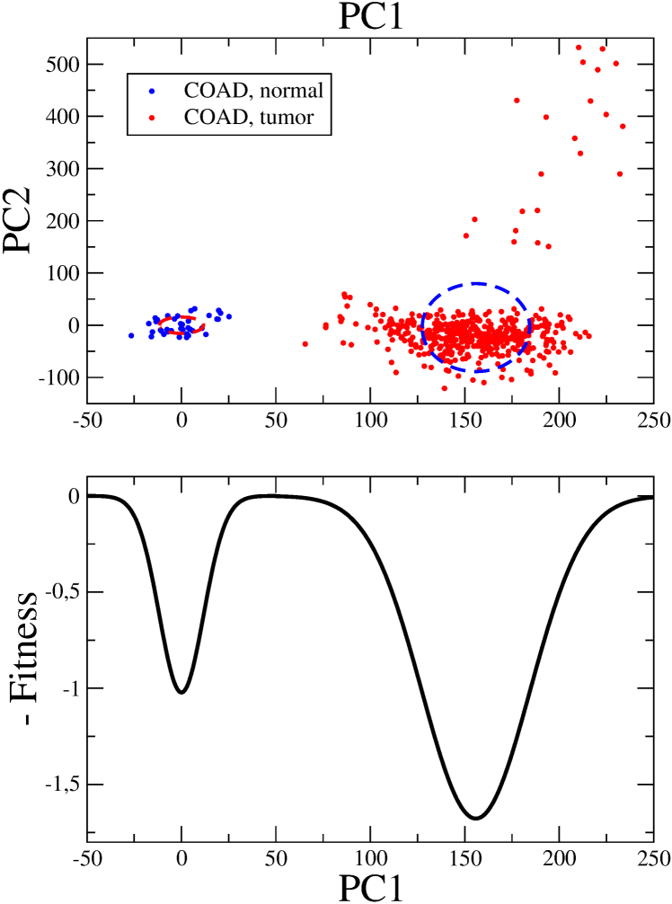
Figure 1: Top: PC analysis of the GE data for adenocarcinoma of the colon. Normal (blue circles) and tumor samples (red circles) are shown. Ellipses illustrating the centers and r.m.s. radi of both clouds of points are drawn. Bottom: Schematics of the fitness landscape. The fitness is normalized to the homeostatic value. The tumor region exhibits the deepest well (highest fitness).

A 1D model for tumorigenesis. We are closer than ever to modeling tumorigenesis. Perhaps, the best way to proceed is to use a gene expression (GE) description [1]. Indeed, in GE space the normal (homeostatic) and tumor states are seen as distant regions (attractors) [2]. Recall, for example, the principal component analysis [3, 4, 5] of GE data for colon adenocarcinoma (COAD), obtained from The Cancer Genome Atlas portal (https://www.cancer.gov/tcga). Fig 1 top panel shows the results [2].

Each point in this figure comes from a biopsy, Small samples are taken off from different patients and processed in order to obtain expression values for 60483 genes. For each gene, we define a reference value, $e_{ref}$, by geometric averaging over the normal samples. Then, new variables are defined: $\hat{e}=\log_{2}(e/e_{ref})$. The origin of coordinates in this figure is precisely the center of the cloud of normal samples, $\hat{e}=0$. A covariance matrix is defined and diagonalized. The first eigenvectors are used to define new coordinate axes: PC1, PC2, etc. Details may be found in Ref. [2]. We shall only stress that the first axis, PC1, which accounts for 51 % of the total data variance, is the cancer axis, which allows the discrimination between normal and tumor states.

Let ${\bf v_{1}}$ be the eigenvector of the covariance matrix along PC1, and ${\bf\hat{e}}$ the expression vector corresponding to a given sample. Then, $x_{1}={\bf\hat{e}\cdot v_{1}}$ is the position along PC1 of the sample. Normal samples define a region around the origin with r.m.s. radius $R_{n}=11.71$. On the other hand, the cloud of tumor samples is centered at $\bar{x}_{1}=155.89$, and its r.m.s. radius is $R_{t}=28.53$ [6].

Recall the interpretation of points in Fig. 1 top panel. Each point comes from a small sample, the GE data obtained from it contains the contribution of many cells and the complex signaling system regulating their interactions. One may speak of a tissue microstate. On the other hand, points come from different patients, each carrying a particular genetic load. The fact that the points are grouped in definite regions means that these regions are indeed attractors in GE space.

We want to describe the genesis of a tumor, that is the time evolution of a portion or sample of a tissue that starts in the normal region and progress towards the tumor zone. We have already defined a single coordinate describing this progression: $x_{1}$. In order to proceed further with the model, we shall clarify why and how this progression takes place.

The coordinate $x_{1}$ describing the tissue microstate starts at a point near the origin and realizes random oscillations in the normal zone. The cause for such random displacements is discussed in the next sections. The motion is confined to the normal region for a long time because this zone is a local maximum of fitness [6, 7]. We have schematically represented in Fig. 1 bottom panel the fitness distribution along the PC1 axis. The $y$ axis of this figure is the fitness with a minus sign, thus that the normal and tumor zones are local maxima. We have computed in Ref. [7] the number of available microstates in each zone, showing that this number is much greater for tumors than for normal states. In other words, the volume of the basin of attraction is much greater in the tumor than in the normal region. In addition, as a consequence of breaking the restrictions imposed by homeostasis, the mitotic rate of tumor stem cells is usually greater than that of normal somatic stem cells [8]. The conclusion is that the tumor minimum is the deepest in Fig. 1, the one with highest fitness. Our drawing for the fitness distribution is a sketch, but we are convinced that at least a rough quantitative description can be reached.

The intermediate region, $R_{n}<x_{1}<\bar{x}_{1}-R_{t}$, holds a low-fitness barrier [6, 7], which prevents the spontaneous transitions from the normal to the tumor region. The relative scarcity of samples in this region evidences the existence of the barrier.

A tissue microstate realizes random displacements within the normal region. Only when the barrier is surpassed and the microstate leaves the normal basin of attraction it is driven towards the tumor attractor. The transition is seen as discontinuous [6].

A precise description of the transition requires the detailed knowledge of the fitness landscape and the causes of the random fluctuations. However, in order to estimate the risk of cancer in a tissue we may proceed in a simpler way and compute the probability for the $x_{1}$ variable describing the microstate to transit from the normal to the tumor region. The minimal walk length is $\bar{x}_{1}-R_{n}-R_{t}$. This is the goal we are aimed at in the present paper.

The starting point in our model is a large set of samples or microstates located near the origin of Fig. 1. They represent small portions of the healthy tissue. We may think of colon crypts in the studied example. The mean number of crypts in a healthy individual is estimated as $1.5\times 10^{7}$ [9]. We shall follow the random oscillations in GE space of each of these crypts.

With regard to the time variable, it is natural to follow the renewal cycle of somatic stem cells, guaranteeing crypt homeostasis. In the studied example, the renewal rate is 73 per year [10]. Thus, we shall measure time in terms of somatic stem cell generations. $t=0$ may refer to conception or to the moment at which the first colon stem cell appears. On the other hand, $t_{0}=\log_{2}N_{sc}$, where $N_{sc}$ is the number of stem cells in the tissue, is the moment at which the tissue is formed. In colon, $N_{sc}\approx 2\times 10^{8}$, and $t_{0}\approx 27$. This is our starting point.

Small random displacements in GE space. Small variations of GE levels spontaneously occurs and may have different origins. First, somatic mutations in the human genome are known to occur at a rate of 8 per cell generation [11]. Second, there is also a rate of accumulation of epigenetic (mainly methylation and phosphorylation) events modifying the normal expression levels [12]. Both processes could be boosted by inherited mutations [13, 14] or external carcinogens [15].

We may thus write for the $x_{1}$ coordinate, characterizing the microstate of a crypt at time $t=n+1$, the following equation:

$$x_{1}^{(n+1)}=x_{1}^{(n)}+\delta x_{1},$$ (1)

where

$$\delta x_{1}={\bf v_{1}\cdot\delta\hat{e}}=\sum_{i}v_{1i}~{}\delta\hat{e}_{i},$$ (2)

and $\delta\hat{e}_{i}$ corresponds to a random variation of the expression of gene i. Eq. (1) describes a Markov chain of events [16]. On the other hand, Eq. (2) shows that fluctuations in the expression levels are filtered by the ${\bf v_{1}}$ vector.

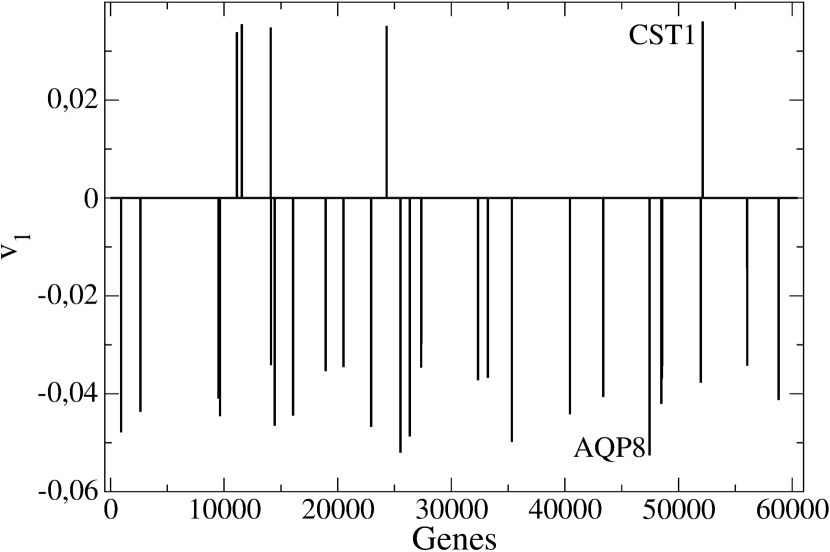
Figure 2: The 30 genes with most significant contributions to the ${\bf v_{1}}$ vector in COAD. CST1 is stressed among the over-expressed and AQP8 among the silenced genes.

In Fig. 2 we draw the 30 genes with the greatest contributions to ${\bf v_{1}}$ in COAD [2]. $v_{1i}>0$ and $v_{1i}<0$ correspond, respectively, to genes that should be over- and under-expressed (silenced) in order to the tumor to progress. We have distinguished the genes CST1 and AQP8. The former is a known marker of colon cancer [17], whereas the latter plays a significant role in colon homeostasis [18] and should be silenced in tumors.

The maximum value of $|v_{1i}|$ defines a scale, $D$, for the fluctuations of $x_{1}$. In COAD, it coincides with the modulus of the $v_{1i}$ related to the AQP8 gene. In order to get a simple estimate for the cancer risk, we may adopt the following model for the fluctuations: $\delta x_{1}=D~{}r$, where $r$ is a uniformly distributed random number in (-1,1). This model may result from an independent variation hypothesis, i.e. random amplitudes and signs in the individual gene variations $\delta\hat{e}_{i}$, so that most of they cancel. In this way, Eq. (1) for the small displacements in GE space describes a 1D Brownian or Poisson process [19].

We may use the well known fact that in a Brownian process, the final amplitudes at a given time are normally distributed, i.e. the probability density is given by:

$$p(x)=\sqrt{a/\pi}~{}e^{-a(x-x_{0})^{2}},$$ (3)

where $a=2/(D^{2}t)$. We shall evaluate the probability for a trajectory starting in the normal zone to reach the tumor zone. Above, we pointed out that the minimal walk length is $R=\bar{x}_{1}-R_{n}-R_{t}$. Thus, an estimate for the risk may be obtained from:

$$\int_{R}^{\infty}p(x){\rm d}x=Err(\sqrt{aR^{2}}),$$ (4)

where $Err$ is the complementary error function. The argument of this function is $z=\sqrt{aR^{2}}=\sqrt{2/t}~{}R/D$, in principle a large number. Then, we may use the asymptotic behavior $Err(z)\approx\exp(-z^{2})/(\sqrt{\pi}z)$ for large $z$. The risk of cancer in COAD is obtained by multiplying the escape probability for a single crypt by the number of crypts, or by the number of stem cells, which is proportional to it:

$$risk\sim N_{sc}~{}\frac{D\sqrt{t}}{R}~{}e^{-2(R/(D\sqrt{t}))^{2}},$$ (5)

or

$$ln(risk/N_{sc})=const+ln(D\sqrt{t}/R)-2(D\sqrt{t}/R)^{-2}.$$ (6)

This expression is general enough to be applied to other tissues, besides colon. The constant in Eq. (6) may account for other effects as, for example, the role of the immune system. Microregions escaping the normal region and forming a proto-tumor could be the subject of an attack by the immune system in the very early stages [20]. By definition, the constant is less than zero because the overall constant in Eq. (5) is less than one.

In Table 1 we compile a set of parameters for a group of tumors. The geometry of the normal and tumor regions, i.e. the parameters $\bar{x}_{1}$, $R_{n}$ and $R_{t}$ come from Ref. [6]. The $D$ value is estimated as the maximum of $|v_{1i}|$ [2]. On the other hand, the number of tissue stem cells, $N_{sc}$, the stem cell turnover rate. $m_{sc}$, and the lifetime risk of cancer (when available) are borrowed from Refs. [21, 22]. The reported values of risk represent averages over 380 cancer registries from different cities and countries in the world [22].

We may test Eq. (6) for the risk of cancer in a tissue resulting from small random variations of GE levels by using the data included in Table 1. A plot of the l.h.s. vs the r.h.s. of Eq. (6) should lead to a straight line with a slope near one and a constant less than zero. Notice that the life expectancy in Ref. [21] is assumed to be 80 years. Thus, $t$ is obtained by multiplying the stem cell rate, $m_{sc}$, by 80 years.

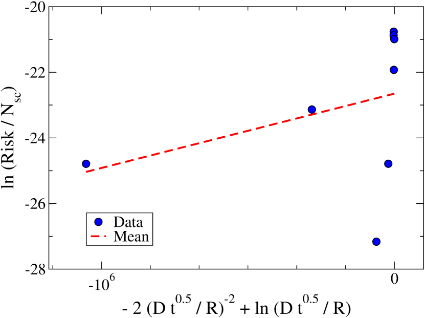
Figure 3: A test of how Eq. (6) describes the risk of cancer in 8 tissues. Data from Table 1 is used to this end. A nearly flat dependence on the abcisa is obtained, thus small amplitude fluctuations in gene expression space may not account for the risk of cancer in these tissues..

The results of that test are shown in Fig. 3. We get a nearly flat curve (slope = $2\times 10^{-6}$), indicating that the proposed dependence of the risk on the parameters is not correct. Thus, the observed risk of cancer can not be explained by small amplitude random variations in GE values. In the next section, we shall consider large jumps.

Let us stress that we use an expression like $t=m_{sc}\times age$ in a very broad age interval. It is well known that $m_{sc}$ experiences a significant decrease as a result of aging [23, 24]. However, also as a consequence of aging there is an accumulation of epigenetic events and DNA damages leading to a reduction of fitness and a displacement towards the low-fitness zone. Thus, aging acts in the same direction as the low amplitude fluctuations of GE values.

Large (Levy) jumps in GE space. Besides small random displacements, related to quasi independent variations in the GE values, there is also the possibility of large jumps in GE space. The origin of such large motions could be diverse.

First, there are large scale mutations, involving DNA rearrangements and simultaneously modifying the expression of many genes. An example, known to play an important role in cancer, is that of aneuploidies [25].

Second, large jumps in GE space could be related to coordinated variations in a group of genes. Indeed, GE values are known to be regulated by GE networks [26]. The global states of these networks define attractors. Variations in genes playing a decisive role in the network, or accumulation of variations in many genes, may cause a transition from one of these global states to another one.

Third, there is also the possibility of a programmed chain of mutations and GE variations leading to cancer, triggered by let unknown causes, which is the basic hypothesis in the atavistic theory of cancer [27].

For the large GE variations, we shall specify their rate of occurrence, $\mu$, and the probability distribution for their amplitudes, $\pi(\Delta x_{1})$.

It is very plausible to assume that $\pi$ is of Pareto [28] or Levy [29] kind, with a power-like tail. Indeed, the Pareto character of GE distribution functions was demonstrated in Ref. [30] (see also [6]). The Levy character of the length distribution functions in mutations was shown in [31].

Thus, our assumption is that displacements in GE space are a kind of Levy flights. Small variations allow the exploration of the fitness landscape at lower scales, whereas sporadic large jumps allow to find global maxima. Besides mutations [31], Levy flights are known to take place in many other biological processes, for example foraging [32].

For lage $|\Delta x_{1}|$, the tail of $\pi$ is described by a Pareto exponent $\nu$:

$$\pi(\Delta x_{1})\sim 1/|\Delta x_{1}|^{\nu}.$$ (7)

The probability of a large jump reaching the tumor region is thus proportional to

$$D~{}(\mu t)~{}\int_{R}^{\infty}{\rm d}x/x^{\nu},$$ (8)

and the risk of cancer in a tissue:

$$risk\sim N_{sc}D~{}\mu~{}(t_{0}+m_{sc}\times age)/R^{\nu-1},$$ (9)

where we assume $\nu>1$. Below, we use $\nu=2$ in order to get an estimate of the risk.

Let us examine Eq. (9) in more details. First, Eq. (8) assumes that $R$ is in the tail of the distribution function. This is justified if we compare $R=115.65$ with the scale $D=0.0526$. Second, no more than one hit or large jump is assumed to occur in the evolution of each microstate. In other words, the probability $\mu t$ is less than one and large jumps are thought to be rare. Third, we should consider the possibility of large GE variations due to mutations in the development period, that is why we included $t_{0}=\log_{2}(N_{sc})$ in the formula. This is particularly important in tissues with slow renewal rates but large number of stem cells. For example, in lung $t_{0}\approx 30$, but $m_{sc}\times 80$ years is only 5.6. Fourth, the rate of large jumps, $\mu$, is unknown. However, if we assume roughly the same value for all tissues, then it can be absorbed in the overall constant entering Eq. (9). The Pareto exponent is also unknown. Notice that in the COAD GE distribution functions the exponents take values between 1.6 and 2.0 [6]. The value we use for estimates, $\nu=2$, is motivated by this result.

Finally, we get the following expression for the risk, which may be tested against the data in Table 1:

$$ln(risk/N_{sc})=const+ln\{D(t_{0}+m_{sc}\times age)/R\}.$$ (10)

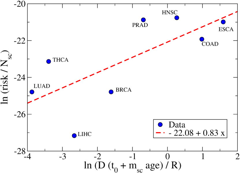
Figure 4: Testing the ability of Eq. (10) to describe the cancer risk in 8 tissues. The slope of the linear fit is near one, as expected. 72 % of the data dispersion is explained by the linear dependence (p-value = 0.04).

The constant should be negative according to our hypothesis of $\mu$ small. The results of the test are shown in Fig. 4.

The observed behavior is consistent with a linear dependence with slope near one. The Pearson correlation coefficient is 0.85, with a p-value equal to 0.04. The main reason for the remaining dispersion of points could be the assumption that the rate of large jumps, $\mu$, is roughly the same for all of the tumors. A variable $\mu$ would account for the dispersion.

In conclusion, we get the following simple expression for the risk of cancer per stem cell in a tissue, coming from large jumps in GE space:

$$\frac{risk}{N_{sc}}=\mu^{\prime}\frac{D}{R}(t_{0}+m_{sc}~{}age),$$ (11)

where we included an effective rate, $\mu^{\prime}$. Genetic, viral or external carcinogenic factors may increase $\mu^{\prime}$, whereas the action of the immune system in the tissue may modify $\mu^{\prime}$ in any direction. In the next section, we qualitatively analyze a larger set of tumors by using Eq. (11).

Qualitative analysis of the data on cancer risk in different tissues. We use Eq. (11) in order to re-examine the data presented in paper [21]. The qualitative idea is to set a reference value for the coefficient in front of the r.h.s. of Eq. (11), $a_{ref}=2\times 10^{-14}$, and include an extra risk score (ERS), in such a way that:

$$\frac{risk}{N_{sc}}=ERS~{}a_{ref}~{}(t_{0}+m_{sc}age).$$ (12)

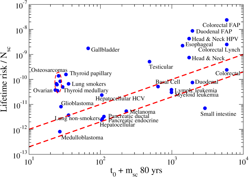
Figure 5: (Color online) Lifetime risk of cancer per stem cell in a tissue vs the number of stem cell generations. The analysis is based on Eq. (12). See the explanation in the main text.

We should try to understand the observed values of ERS in terms of the tissue characteristics. The results are shown in Fig. 5. In order to facilitate the analysis, the studied tumors are separated in groups.

Group I includes 11 tumors (9 tissues), located in a band delimited by red dashed lines in Fig. 5, and coefficients $1<ERS<5$. In the lack of a better name, it is called the normal group. In this set, random fluctuations in GE space seem to play the main role in the genesis of cancer, as originally claimed in Ref. [21]. Notice that this group is conformed by very different tissues – from the medulloblastoma to the colorectal adenocarcinoma.

Group II, with five points in the figure, include cases in which genetic or viral causes enhance the rate $\mu^{\prime}$. The ERS index exhibits very high values in this set.

The abnormal values of ERS for the 7 tissues (12 points) contained in Group III could have an immunological origin. Indeed, our body uses physical barriers, humors and immune cells in order to protect the tissues against infections caused by pathogens, which are the most common attacks. The combined effects of these factors guarantees immunity. In tissues where one factor is predominant, the others could be somehow depressed. On the other hand, the protection against tumors, which come form inside, that is originate in tissue cells, is mainly the responsibility of immune cells.

Barriers are known to play a basic role in the protection of germinal cells [33] and the brain [34] against infections. The cellular component of immunity in these tissues is, in some way, depressed with the purpose of avoiding inflammation events. The relatively high values of ERS could be explained in this way.

By contrast, the inclusion of the Medulloblastoma in the normal group is probably related to regional differences in blood-brain barrier permeability [35].

With regard to bones, it is known that immunity relies strongly on defensins [36], possibly with a depressed role of immune cells. On the other hand, the thyroid is known to have a close cross-talk with the immune system [37]. It’s dysregulation is the cause of immune disorders. One may speculate that a low cellular response is needed in order to prevent dysregulation of the thyroid.

The extreme case in this group is gallbladder non-papillary adenocarcinoma, with an index $ERS=1300$, the understanding of which is a real challenge. However, one can speculate that the cellular response is also depressed in the gallbladder, because of the strong microbicide character of the bile [38].

On the other hand, the relatively low value of ERS for the small intestine adenocarcinoma (eight times lower than the reference) can not have other explanation than overprotection by the cellular component of the immune system. Indeed, the small intestine is a possible entrance door for the microbiota living in the colon, and as such it requires special protection. The mean value of microbes/gm experiences a jump from $10^{4}$ to $10^{11}$ as we cross from the ileum to the cecum [39]. Barriers can not be reinforced because of the reduced dimensions. Thus, perhaps the Paneth cells [40], Peyer’s patches [41], and other structures concentrated in the distal ileum are the responsible for this additional protection.

Finally, there is a group of 3 tissues exhibiting abnormally high values of the ERS index, presumably related to external factors. One example is lung adenocarcinoma, for which the concurrence of radioactive Radon and smoking produces a 90-fold increase of the slope.

Concluding remarks. In the present paper, the time evolution of microstates representing small portions of a tissue are described as Levy flights in gene expression space. The small amplitude Brownian component is characterized by a radius $D\sqrt{t}$, much less than the distance between the normal and tumor regions, $R=\bar{x}_{1}-R_{n}-R_{t}$. Only sporadic large jumps, of Levy nature, allow the microstate to reach the cancer basin of attraction.

Although it is understood that aging induces a motion in the direction of the low-fitness region, it was not explicitly included in our model. Work along this direction is necessary.

The resulting formula for the risk of cancer in a tissue was quantitatively tested against observed data, and applied to the qualitative analysis of the risk of cancer in a set of tissues. The most important conclusion, in our opinion, is a possible connection between the risk and the way the tissue is protected against infections. The blood-brain barrier in the cerebrum, for example, preventing the entrance of pathogens, is also the reason for the relatively low rate of elimination of prototumors, and thus large risk per stem cell in this organ. The low risk per stem cell in the small intestine, on the other hand, is understood as a reinforcement of the cellular component of immunity.

Acknowledgments. A.G. acknowledges the Cuban Program for Basic Sciences, the Office of External Activities of the Abdus Salam Centre for Theoretical Physics, and the University of Electronic Science and Technology of China for support. The research is carried on under a project of the Platform for Bioinformatics of BioCubaFarma, Cuba.

Tissues	$\bar{x}_{1}$	$R_{n}$	$R_{t}$	$R$	$D$	$N_{sc}$	$m_{sc}$ (1/yr)	risk
BRCA	137.37	20.97	31.66	84.74	0.0450	$6.5\times 10^{9}$	4.3	0.1116
COAD	155.89	11.71	28.53	115.65	0.0526	$2\times 10^{8}$	73	0.0601
HNSC	123.50	27.74	23.54	72.22	0.0549	$1.85\times 10^{7}$	21.15	0.0178
KIRC	171.80	28.70	36.00	107.1	0.0679	…	…	…
KIRP	163.42	19.90	27.78	115.74	0.0768	…	…	…
LIHC	134.67	20.48	45.23	68.96	0.0461	$3.01\times 10^{9}$	0.9125	0.0048
LUAD	145.33	13.51	32.06	99.76	0.0581	$1.22\times 10^{9}$	0.07	0.0209
LUSC	194.49	11.62	36.65	146.22	0.0522	…	…	…
PRAD	91.33	31.31	32.17	27.85	0.0523	$2.1\times 10^{8}$	3	0.1804
STAD	136.97	27.14	43.24	66.59	0.0455	…	…	…
THCA	112.54	20.02	39.85	52.67	0.0532	$8.25\times 10^{7}$	0.087	0.0074
UCEC	171.38	38.24	22.14	111.00	0.0439	…	…	…
BLCA	140.61	57.53	34.68	48.40	0.0512	…	…	…
ESCA	138.70	64.28	35.79	38.63	0.0710	$6.65\times 10^{6}$	33.18	0.0051
READ	168.05	22.90	28.81	116.34	0.0521	…	…	…

Table 1: A set of parameters compiled for a group of tumors. The geometry of the normal and tumor regions, i.e. the parameters $\bar{x}_{1}$, $R_{n}$ and $R_{t}$ come from Ref. [6]. The minimal distance between both regions is $R=\bar{x}_{1}-R_{n}-R_{t}$. The $D$ value is estimated as the maximum of $|v_{1i}|$ [2]. On the other hand, the number of tissue stem cells, $N_{sc}$, the stem cell turnover rate. $m_{sc}$, and the lifetime risk of cancer (when available) are borrowed from Refs. [21, 22].

Cancer type	ERS
Group I. Normal
Hepatocellular C	1.13
Melanoma	1.16
Pancreatic endocrine C	1.23
Pancreatic ductal AC	1.45
Medulloblastoma	1.49
Myeloid leukemia	1.54
Duodenal AC	1.93
Lymphocytic leukemia	1.95
Colorectal AC	2.04
Basal Cell C	4.02
Lung AC (non-smokers)	5.15
Group II. Viral and Genetic
Hepatocellular C with HCV	11.29
Colorectal AC with Lynch	21.30
Head and Neck SCC with HPV	122.96
Colorectal AC with FAP	204.51
Duodenal AC with FAP	225.29
Group III. Immune
Small intestinal AC	0.12
Glioblastoma	14.48
Testicular germinal cell	52.78
Ovarian germinal cell	79.86
Thyroid medullary C	84.22
Osteosarcomas	153.04
Thyroid papillary and follicular C	239.78
Gallbladder non papillary AC	1299.58
Group IV. Abnormal
Head and Neck SCC	21.38
Esophageal SCC	79.44
Lung AC (smokers)	92.77

Table 2: The Extra Risk Score (ERS) index of Eq. (12) for cancer in different tissues.

References

- [1] U. Alon, N. Barkai, D. A. Notterman, K. Gish, S. Ybarra, D. Mack, and A. J. Levine. Broad patterns of gene expression revealed by clustering analysis of tumor and normal colon tissues probed by oligonucleotide arrays. PNAS, 96 (12):6745–6750, 1999.
- [2] Augusto Gonzalez, Yasser Perera, and Rolando Perez. On the gene expression landscape of cancer. (unpublished). 2020.
- [3] Svante Wold, Kim Esbensen, and Paul Geladi. Principal component analysis. Chemometr. Intell. Lab. Syst., 2(1-3):37–52, 1987.
- [4] Jake Lever, Martin Krzywinski, and Naomi Altman. Principal component analysis. Nat. Methods, 14:641–642, 2017.
- [5] Markus Ringner. What is principal component analysis? Nat. Biotechnol., 26:303–304, 2008.
- [6] Augusto Gonzalez, Joan Nieves, Maria Luisa Bringas, and Pedro Valdes-Sosa. Gene expression rearrangements denoting changes in the biological state. (unpublished). 2020.
- [7] Frank Quintela and Augusto Gonzalez. Estimating the number of available states for normal and tumor tissues in gene expression space. (unpublished). 2020.
- [8] Sten Friberg and Stefan Mattson. On the growth rates of human malignant tumors: Implications for medical decision making. J. Surg. Oncol., 65 (4):284–297, 1997.
- [9] B. M. Boman, J. Z. Fields, K. L. Cavanaugh, A. Guetter, and O. A. Runquist. How dysregulated colonic crypt dynamics cause stem cell overpopulation and initiate colon cancer. Cancer Res., 68 (9):3304–13, 2008.
- [10] R. Okamoto and M. Watanabe. Molecular and clinical basis for the regeneration of human gastrointestinal epithelia. J. Gastroenterol., 39 (1):1–6, 2004.
- [11] Brandon Milholland, Xiao Dong, Lei Zhang, Xiaoxiao Hao, Yousin Suh, and Jan Vijg. Differences between germline and somatic mutation rates in humans and mice. Nat. Commun., 8 (1):15183, 2017.
- [12] Keith D. Robertson. Dna methylation and human disease. Nat. Rev. Genet., 6 (8):597–610, 2005.
- [13] Mary-Claire King, Joan H. Marks, and Jessica B. Mandell. Breast and ovarian cancer risks due to inherited mutations in brca1 and brca2. Science, 302 (5645):643–646, 2003.
- [14] Julian R. Sampson, Sunil Dolwani, Sian Jones, Diana Eccles, Anthony Ellis, D. Gareth Evans, Ian Frayling, Sheila Jordan, Eamonn R. Maher, Tony Mak, Julie Maynard, Francesca Pigatto, Joan Shaw, and Jeremy P. Cheadle. Autosomal recessive colorectal adenomatous polyposis due to inherited mutations of myh. Lancet, 362 (9377):39–41, 2003.
- [15] Jessica L. Barnes, Maria Zubair, Kaarthik John, Miriam C. Poirier, and Francis L. Martin. Carcinogens and dna damage. Biochem. Soc. Trans., 46 (5):1213–1224, 2018.
- [16] V. S. Koroliuk, N. I. Portenko, A. V. Skorojod, and A. F. Turbin. Handbook on probability theory and mathematical statistics. Nauka, Moscow, 1978.
- [17] Taiyuan Li, Qiangqiang Xiong, Zhen Zou, Xiong Lei, Qunguang Jiang, and Dongning Liu. Prognostic significance of cystatin sn associated nomograms in patients with colorectal cancer. Oncotarget, 8 (70):115153–115163, 2017.
- [18] Celia Escudero-Hernandez, Andreas Munch, and Ann-Elisabet Ostvik. The water channel aquaporin 8 is a critical regulator of intestinal fluid homeostasis in collagenous colitis. J. Crohns Colitis, jjaa020, 2020.
- [19] A. Einstein. Investigations on the theory of the brownian movement. New York: Dover Publications, Inc., page 124, 1956.
- [20] Wolf H. Fridman, Laurence Zitvogel, Catherine Sautès-Fridman, and Guido Kroemer. The immune contexture in cancer prognosis and treatment. Nat. Rev. Clin. Oncol., 14 (12):717–734, 2017.
- [21] C. Tomasetti and B. Vogelstein. Variation in cancer risk among tissues can be explained by the number of stem cell divisions. supplementary materials at www.sciencemag.org/content/347/6217/78/suppl/. Science, 347:78–81, 2015.
- [22] C. Tomasetti and B. Vogelstein. Stem cell divisions, somatic mutations, cancer etiology, and cancer prevention. Science, 355 (6331):1330–1334, 2017.
- [23] Valerie D. Roobrouck, Fernando Ulloa-Montoya, and Catherine M. Verfaillie. Self-renewal and differentiation capacity of young and aged stem cells. Exp. Cell Res., 314 (9):1937–1944, 2008.
- [24] A. S. Ahmed, M. H. Sheng, Wasnik S., Baylink D. J., and Lau K. W. Effect of aging on stem cells. World J. Exp. Med., 7 (1):1–10, 2017.
- [25] Ithamar Ganmore, Gil Smooha, and Shai Izraeli. Constitutional aneuploidy and cancer predisposition. Human Molecular Genetics, 18 (R1):R84–R93, 2009.
- [26] Frank Emmert-Streib, Matthias Dehmer, and Benjamin Haibe-Kains. Gene regulatory networks and their applications: understanding biological and medical problems in terms of networks. Front. Cell. Dev. Biol., 2:38, 2014.
- [27] Luis Cisneros, Kimberly J. Bussey, Adam J. Orr, Milica Miocevic, Charles H. Lineweaver, and Paul Davies. Ancient genes establish stress-induced mutation as a hallmark of cancer. Front. Cell. Dev. Biol., 12 (4):e0176258, 2017.
- [28] M.E.J. Newman. Power laws, pareto distributions and zipf’s law. Contemporary Physics, 46 (5):323–351, 2005.
- [29] M. F. Shlesinger, G. Zaslavsky, and U. (Eds.) Frish. Levy flights and related phenomena in physics, lecture notes in physics. Springer, Berlin, 450, 1995.
- [30] V. A. Kuznetsov, G. D. Knott, and R. F. Bonner. General statistics of stochastic process of gene expression in eukaryotic cells. Genetics, 161 (3):1321–1332, 2002.
- [31] D. A. Leon and A. Gonzalez. Mutations as levy flights. (unpublished). 2020.
- [32] N. E. Humphries and D. W. Sims. Optimal foraging strategies: Levy walks balance searching and patch exploitation under a very broad range of conditions. J. Theor. Biol., 358:179–193, 2014.
- [33] L. R. França, S. A. Auharek, R. A. Hess, J. M. Dufour, and B. T. Hinton. Blood-tissue barriers: morphofunctional and immunological aspects of the blood-testis and blood-epididymal barriers. Adv. Exp. Med. Biol., 763:237–259, 2012.
- [34] Nina M. van Sorge and Kelly S. Doran. Defense at the border: the blood–brain barrier versus bacterial foreigners. Future Microbiol., 7 (3):383–394, 2012.
- [35] Timothy W. Phares, Rhonda B. Kean, Tatiana Mikheeva, and D. Craig Hooper. Regional differences in blood-brain barrier permeability changes and inflammation in the apathogenic clearance of virus from the central nervous system. J. Immunol., 176 (12):7666–7675, 2006.
- [36] D. Varoga, C. J. Wruck, M. Tohidnezhad, L. Brandenburg, F. Paulsen, R. Mentlein, A. Seekamp, L. Besch, and T. Pufe. Osteoblasts participate in the innate immunity of the bone by producing human beta defensin-3. Histochem Cell. Biol., 131 (2):207–218, 2008.
- [37] Cristiana Perrotta, Clara De Palma, Emilio Clementi, and Davide Cervia. Hormones and immunity in cancer: are thyroid hormones endocrine players in the microglia/glioma cross-talk? Front. Cell Neurosci., 9:236, 2015.
- [38] M. E. Merritt and J. R. Donaldson. Effect of bile salts on the dna and membrane integrity of enteric bacteria. J. Med. Microbiol., 58 (Pt 12):1533–1541, 2009.
- [39] A. M. O’Hara and F. Shanahan. The gut flora as a forgotten organ. EMBO Rep., 7 (7):688–693, 2006.
- [40] Hans C. Clevers and Charles L. Bevins. Paneth cells: maestros of the small intestinal crypts. Annual Review of Physiology, 75 (1):289–311, 2013.
- [41] Camille Jung, Jean-Pierre Hugot, and Frederick Barreau. Peyer’s patches: The immune sensors of the intestine. Int. J. Inflam., 2010:823710, 2010.