Numerical study of the unitary Fermi gas across the superfluid transition

Abstract

We present results from Monte Carlo calculations investigating the properties of the homogeneous, spin-balanced unitary Fermi gas in three dimensions. The temperature is varied across the superfluid transition allowing us to determine the temperature dependence of the chemical potential, the energy per particle and the contact density. Numerical artifacts due to finite volume and discretization are systematically studied, estimated, and reduced.

I Introduction

Ultracold, dilute gases of fermionic atoms have been studied extensively lately, in part due to the system being the simplest environment with strong interactions between fermions (for recent reviews of this active field see e.g. Refs. Giorgini et al. (2008); Zwerger (2012)). Most remarkably, a three-dimensional (3d) atomic gas with two hyperfine states, say lithium or potassium, can be constructed to have resonant interactions: by applying an external magnetic field the S-wave scattering length $a$ can be tuned to satisfy $1/a=0$. In this special situation, the properties of the gas become universal, dependent only on the density and temperature. What can be learned in the atomic physics laboratory then has implications for nonrelativistic fermions as small as nucleons.

This resonant Fermi gas – often called the “unitary Fermi gas” due to the scattering being limited only by unitarity – provides an excellent opportunity for quantitative theoretical calculations. The clean separation of scales means that much can be inferred from dimensional analysis and scaling arguments. What remains to be determined are universal dimensionless constants, such as the Bertsch parameter Bishop (2001), or functions of the product of the inverse temperature $\beta$ and the chemical potential $\mu$ Ho (2004) which completely specify the thermodynamic and hydrodynamic behavior of the unitary Fermi gas. Much effort has gone into using first-principles numerical methods to determine these quantities (see Refs. Pollet (2012); Lee (2009); Drut and Nicholson (2013) for reviews).

In this paper we use lattice Monte Carlo methods to give numerical results for thermodynamic quantities as the temperature is varied through the superfluid phase transition. In particular we determine the chemical potential, mean energy density, and contact density as functions of temperature. The corresponding universal functions $f(\beta\mu)$ are made dimensionless by taking ratios with the appropriate powers of the Fermi energy $\varepsilon_{F}$. It is notable that several other numerical methods for studying the Fermi gas cannot study the superfluid phase. With this study, we also pay particular attention to investigating and quantifying the systematic uncertainties associated with taking the thermodynamic limit and the continuum limit, which is crucial to obtain correct physical results Privitera et al. (2010); Privitera and Capone (2012). Generally, we find good agreement with experiment.

In previous work Goulko and Wingate (2010a) we used the Diagrammatic Determinant Monte Carlo (DDMC) algorithm Rubtsov et al. (2005); Burovski et al. (2006a, b) to numerically determine the critical temperature $T_{c}$ and thermodynamic properties of the unitary Fermi gas at $T=T_{c}$. Here we study the temperature dependence of physical observables in the approximate range $T_{c}/2\leq T\leq 2T_{c}$. An approach which is formulated in the continuum, bold-line diagrammatic Monte Carlo (bold DMC), has been used to compute quantities above the critical temperature Van Houcke et al. (2012, 2013), and these results agree well with experimental measurements. This method as presently formulated does not extend to temperatures below $T_{c}$ due to the singularity in the pair propagator appearing in the superfluid phase. Temperature effects have also been studied in a lattice computation using a hybrid Monte Carlo approach Drut et al. (2012); however results using different lattice spacings are not presented there.

II Setup

We consider a system of equal-mass fermions with two spin components labeled by the spin index $\sigma=\{\uparrow,\downarrow\}$. Since the details of the physical potential governing the interatomic interactions are irrelevant in the dilute limit realized in cold-atom experiments, we can work on a spatial lattice provided that we also take the dilute limit Chen and Kaplan (2004). The Hamiltonian is that of the simple Fermi-Hubbard model in the grand canonical ensemble,

$$H=\sum_{\mathbf{k},\sigma}(\epsilon_{\mathbf{k}}-\mu_{\sigma})c^{\dagger}_{\mathbf{k}\sigma}c_{\mathbf{k}\sigma}+U\sum_{\mathbf{x}}c^{\dagger}_{\mathbf{x}\uparrow}c_{\mathbf{x}\uparrow}c^{\dagger}_{\mathbf{x}\downarrow}c_{\mathbf{x}\downarrow},$$ (1)

where the first term corresponds to the kinetic part of the Hamiltonian $H_{\rm kin}$ and the second term to the interaction part $H_{\rm int}$. The units are chosen such that $\hbar=k_{B}=2m=1$. We work on a 3d periodic lattice with lattice spacing $b$ and $L^{3}$ sites. The discrete dispersion relation reads $\epsilon_{\mathbf{k}}=2b^{-2}\sum_{j=1}^{3}(1-\cos{k_{j}b})$; $\mu_{\sigma}$ is the chemical potential and $c^{\dagger}_{\mathbf{k}\sigma}$ the fermionic creation operator. The coupling constant $U<0$ corresponding to attractive interaction can be tuned so that the scattering length becomes infinite. The corresponding value in the infinite-volume limit is $U=-7.914/b^{2}$ which is the value we use throughout the calculation. Another approach is to include finite-volume effects in this two-body matching calculation Lee and Schafer (2006); Lee and Schäfer (2006); Drut et al. (2012). It remains to be seen which approach leads to a milder extrapolation of many-body results to the continuum limit.

The partition function $Z=\mathrm{Tr}\exp(-\beta H)$ can be written as a series of products of two matrix determinants built of free finite-temperature Green’s functions Rubtsov et al. (2005). If $\mu_{\uparrow}=\mu_{\downarrow}\equiv\mu$, as is always assumed to be the case in the present work, the two determinants are identical since the spin-dependence enters only via the chemical potential. Consequently all terms in the series are positive, and the series can be used as a probability distribution for Monte Carlo sampling.

We use the DDMC algorithm as introduced in Burovski et al. (2006a) with several modifications which increase the efficiency by reducing autocorrelation effects as compared to the original setup. We account for remaining autocorrelations by binning the data to the point where the statistical error is insensitive to the bin size. A detailed description of our numerical setup is given in Goulko and Wingate (2009, 2010a); Goulko (2011).

We performed many calculations, varying the dimensionless inputs for the chemical potential ($\mu b^{2}$) and inverse temperature ($\beta/b^{2}$), as well as the number of lattice points $L^{3}$, so that controlled extrapolations to the thermodynamic and continuum limits could be taken for a range of temperatures in both the normal and superfluid phases. Each diamond in Fig. 1 represents the thermodynamic limit of lattice calculations done for values of $\mu b^{2}$ and $\beta/b^{2}$ resulting in the corresponding filling factor $\nu$ and dimensionless product $\beta\mu$.

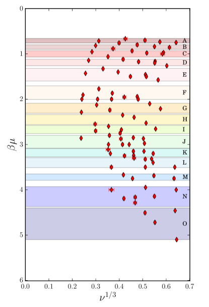
Figure 1: Diamonds correspond to parameters used for individual simulations extrapolated to the thermodynamic limit. The 15 bands indicate the subsets of data included in the continuum ($\nu\to 0$) extrapolations as described in Sec. III.

III Thermodynamic and continuum limits

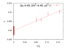
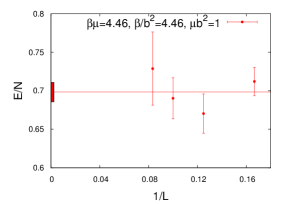
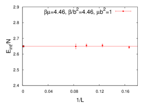
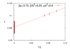
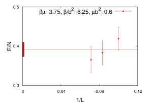
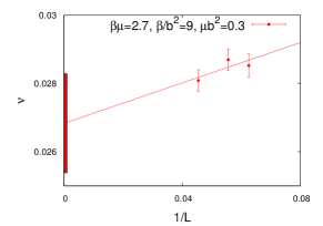
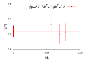
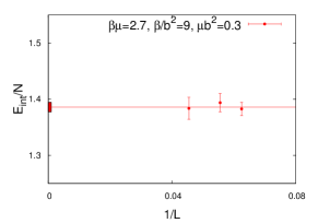
Figure 2: Examples of thermodynamic limit extrapolations in the superfluid phase for the filling factor $\nu$ (left), the energy per particle $E/N=E/L^{3}\nu$ (middle), and the interaction energy per particle $E_{\rm int}/N=E_{\rm int}/L^{3}\nu$ (right), which yields the value of the contact.

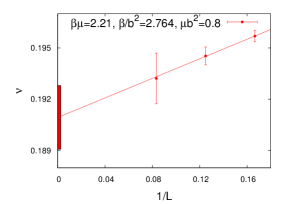
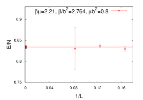
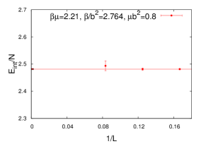
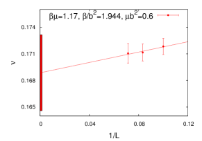
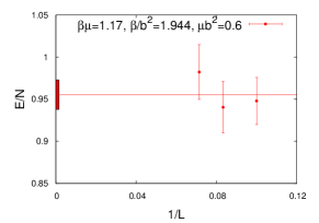
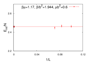
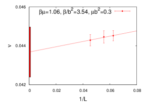
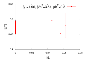
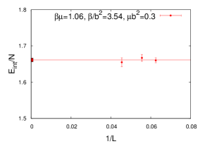
Figure 3: Examples of thermodynamic limit extrapolations in the normal phase for the filling factor $\nu$ (left), the energy per particle $E/N=E/L^{3}\nu$ (middle), and the interaction energy per particle $E_{\rm int}/N=E_{\rm int}/L^{3}\nu$ (right), which yields the value of the contact.

We set the physical scale via $\nu=nb^{3}$, where $\nu=\langle\sum_{\sigma}c^{\dagger}_{\mathbf{x}\sigma}c_{\mathbf{x}\sigma}\rangle$ is the dimensionless filling factor and $n$ the particle number density. Due to universality all physical quantities are given in units which can be expressed as appropriate powers of the Fermi energy $\varepsilon_{\rm F}=(3\pi^{2}n)^{2/3}$. To extract the physical results we need to perform two limits: the thermodynamic limit to infinite system size and then the continuum limit to zero lattice spacing.

First we take the thermodynamic limit in order to estimate and reduce systematic errors due to finite volume. For each $(\mu b^{2},\beta/b^{2})$ we perform computations with several (usually 3 or 4) sizes of cubic volumes, $V=L^{3}$, and extrapolate results as $1/L\to 0$. At the lowest filling factor (smallest $b$) we used volumes up to $V=32^{3}$ (corresponding to up to 1000 particles). Typical ranges are $L=6$ to $L=14$ at higher filling factors (about 40 to 700 particles) and $L=10$ to $L=32$ at lower filling factors (about 100 to 1000 particles). We find that the filling factor $\nu$ is the quantity most sensitive to finite-volume effects. With periodic boundary conditions, we expect finite-volume effects to cause an increase in filling factor compared to the infinite-volume limit. In small volumes the particles will feel an enhanced attraction not just from their neighboring particles, but also from their round-the-world doppelgängers. In agreement with Burovski et al. (2006a) we observe that the data for the filling factor are fit well by a linear function of $1/L$. Once we have $\nu$ in the thermodynamic limit, we can obtain $\varepsilon_{\rm F}$ and the dimensionless observables by taking $\nu$ to the appropriate power and multiplying by quantities which have no statistically significant finite-volume errors. Within the statistical uncertainties, it appears that finite-volume errors are negligible for $E/N$ and $E_{\mathrm{int}}/N$. Examples of thermodynamic extrapolations are shown in Figs. 2 and 3 for different parameter sets in the superfluid and normal phases, respectively.

For the continuum limit we vary the dimensionless chemical potential $\mu b^{2}$ such that the filling factor tends to zero. This is equivalent to $b\rightarrow 0$ since $b\propto\nu^{1/3}$ if $n$ is fixed to be a constant, physical value. Dimensionless ratios of physical quantities can then be extrapolated to the continuum limit by assuming discretization effects can be parametrized using a power series in $b$, or equivalently $\nu^{1/3}$.

Our previous work Goulko and Wingate (2010a, b) focused on determining the critical temperature and computing thermodynamic observables there. The critical temperature was determined at several values of the lattice spacing. In practice this was done by varying the inverse temperature and chemical potential in lattice units to the point where a finite-size scaling study of the order parameter indicated the transition would occur in infinite volume. Here we extend that work by taking the continuum limit of observables for a range of temperatures on either side of the phase transition.

Ideally the continuum limit would be taken varying $b$ along lines of constant $\beta\mu$. The numerical data acquired, however, do not lie exactly along lines of constant $\beta\mu$. Therefore, we group the data in several narrow bands of $y=\beta\mu$ values and extrapolate the data within each band to the continuum limit. Each band is defined by a central value $y_{0}$ and a width, as shown in Fig. 1. In order to account for mild $y$ dependence, we find it sufficient to introduce a term proportional to $\delta y=y-y_{0}$ in the extrapolation function. The lattice spacing dependence of a physical quantity $X$ can be written as a power series in the lattice spacing $b\propto\nu^{1/3}$ Symanzik (1983). Therefore, our continuum limit fits are to functions of the form

$$X(y_{0};\nu,\delta y) =X_{0}\left(1+d_{1}\delta y+\sum_{k=1}^{K}c_{k}\nu^{k/3}\right)\,.$$ (2)

The fit parameter $X_{0}=X_{0}(y_{0})$ is then taken to be the continuum limit result. The other fit parameters, $d_{1}$ and $c_{k}$ also depend on $y_{0}$, but we suppress this dependence in the notation. In almost every case the Monte Carlo data are sufficient to determine $c_{1}$ but not the coefficients of higher-order terms. In other words, the data points indeed look linear in $\nu^{1/3}$. However, given that, especially for larger $y$, the numerical values of $\nu^{1/3}$ are not very small, it is prudent to allow for higher-order contributions in the numerical data. Therefore we introduce Bayesian prior distributions for the $c_{k}$ with $k>1$ Lepage et al. (2002). In the cases where the Monte Carlo results do constrain $c_{2}$ (i.e. fits to $\mu/\varepsilon_{\rm F}$ at low $y$) we find $c_{2}\approx 0.3$. Therefore, we take Gaussian prior distributions centered at 0 with width 0.3. We found very little difference in the fits where we set $K=2$ or $K=3$, but we used the latter, more conservative, option for the results presented here. Finally, we also performed fits which included a term $f_{1}\,\delta y\,\nu^{1/3}$, with a Gaussian prior for $f_{1}$ of $0.0\pm 1.0$. This had no effect on the fits, so for simplicity we omit this term from our final fits.

In Fig. 4 we show the results of these fits for 5 of the 15 bands. The fit curve and corresponding error are evaluated at the value of $\beta\mu$ given in the legend, and represent an interpolation of the data to the central value of the lettered band shown in Fig. 1 as well as the continuum extrapolation to $\nu=0$. In the case of band F, we have several data points generated with $\beta\mu=2$; we emphasize these points with stars. Within uncertainties, the widths of the bands in $\beta\mu$ are sufficiently narrow that interpolating in $\beta\mu$ is mild, well-parametrized by the $d_{1}$ term in Eq. (2).

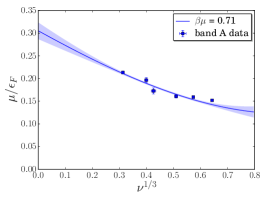
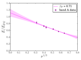
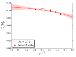
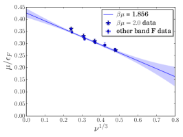
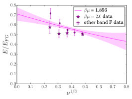
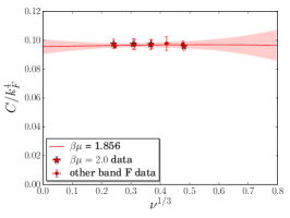
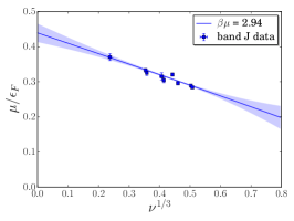
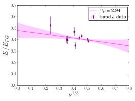
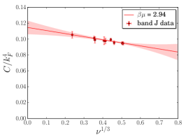
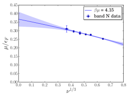
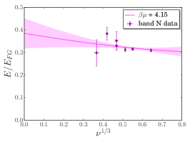
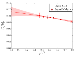
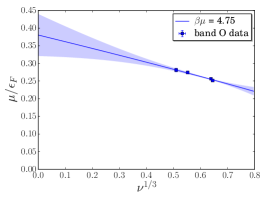
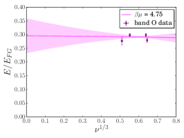
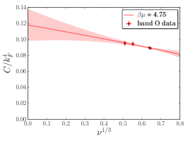
Figure 4: Continuum limit extrapolation along bands of constant $\beta\mu\pm\delta(\beta\mu)$ (see Fig. 1) for the chemical potential (left), energy density (middle) and contact density (right). See further discussion at the end of Sec. III regarding the interpolation in $\beta\mu$.

Summarizing the size of discretization error for the continuum extrapolations, we show the values obtained for the coefficient $c_{1}$ of $\nu^{1/3}$ in Eq. (2). Figure 5 shows that the Monte Carlo data for the chemical potential and energy per particle have significant linear dependence on the lattice spacing, as parametrized by $\nu^{1/3}$, especially at lower $\beta\mu$. This is similar to what was seen for lattice determinations of $T_{c}$ Burovski et al. (2006a); Goulko and Wingate (2010a). Nevertheless, the fits described above, which include possible contributions of higher-order terms, include estimates of these lattice artifacts in the uncertainties quoted below. We tried a variety of other fits, altering the bands in $\beta\mu$, and omitting data with large filling factor, e.g., $\nu^{1/3}>0.5$ Privitera and Capone (2012). These variations produced fits which were in agreement with our final results, but were less precise in some cases.

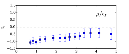
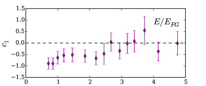
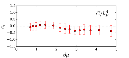
Figure 5: The fit parameter $c_{1}$ obtained from continuum extrapolations, see Eq. (2), of Monte Carlo data for the chemical potential (top), energy per particle (middle), and contact density (bottom).

IV Results

IV.1 Chemical potential

The left panel of Fig. 6 shows the continuum limit of the chemical potential as a function of $\beta\mu$. We see excellent agreement with experimental data Ku et al. (2012); Nascimbène et al. (2010), as well as with several other theoretical predictions Van Houcke et al. (2012); Haussmann et al. (2007). Our results below $T_{c}$ capture the experimentally observed change of the slope of the chemical potential curve.

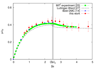
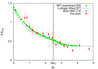
Figure 6: The chemical potential $\mu/\varepsilon_{\rm F}$ (left panel) and the energy per particle $E/E_{\rm FG}$ (right panel) in the continuum limit versus $\beta\mu$. We compare our results (red circles; the empty circles denote our results at $T_{c}$ from Goulko and Wingate (2010a)) with experimental data Ku et al. (2012) (green squares), as well as results obtained with bold DMC Van Houcke et al. (2012) (blue triangles) and with the Luttinger-Ward formalism Haussmann et al. (2007) (black dashed line). The gray bar indicates the critical point Goulko and Wingate (2010a) with error margin.

IV.2 Energy per particle

The energy is composed of the kinetic energy $E_{\textnormal{kin}}$ and the interaction energy $E_{\textnormal{int}}$. We find that, within the statistical uncertainties, neither $E_{\mathrm{kin}}/N$ nor $E_{\mathrm{int}}/N$ exhibit dependence on $L$. This insensitivity can be understood by looking at the lattice Monte Carlo estimator for $E_{\textnormal{kin}}/N=E_{\textnormal{kin}}/L^{3}\nu$ Goulko and Wingate (2010a), which can be expressed as

$$\frac{E_{\textnormal{kin}}}{L^{3}\nu}=6\left(1-\frac{\sum_{\sigma}\langle c^{\dagger}_{\mathbf{x}\sigma}c_{(\mathbf{x}+\hat{\mathbf{j}})\sigma}\rangle}{\nu}\right).$$ (3)

This expression contains the ratio of the kinetic energy operator $\sum_{\sigma}\langle c^{\dagger}_{\mathbf{x}\sigma}c_{(\mathbf{x}+\hat{\mathbf{j}})\sigma}\rangle$ and the filling factor operator $\sum_{\sigma}\langle c^{\dagger}_{\mathbf{x}\sigma}c_{\mathbf{x}\sigma}\rangle$. These two operators have a very similar structure, which explains to some extent why finite-volume errors are negligible within the error bars of the data. The same holds for the interaction part of the energy. Therefore it is sufficient to consider the finite-size scaling of $1/\varepsilon_{\rm F}$ (which follows directly from the finite-size scaling of $\nu$), while the data for $E/L^{3}\nu$ obtained at different lattice sizes can be fitted by a constant. Our data confirms this scaling, as the constant fits of $E/L^{3}\nu$ yield acceptable $\chi^{2}$-values, see the middle panel of Figs. 2 and 3 for several examples.

The results for the energy per particle $E/E_{\rm FG}$, where $E_{\rm FG}=(3/5)N\varepsilon_{\rm F}$ is the ground state energy of the free gas, are shown in the right panel of Fig. 6. Like for the chemical potential, we obtain excellent agreement with experimental data Ku et al. (2012); Nascimbène et al. (2010) and theory Van Houcke et al. (2012); Haussmann et al. (2007).

IV.3 Contact density

The contact density can be interpreted as a measure of the local pair density Braaten (2011). The contact plays a crucial role for several universal relations derived by Tan Tan (2008a, b, c). We use the definition $C=m^{2}g_{0}E_{\textnormal{int}}$, where $g_{0}$ is the physical coupling constant Braaten (2011); Werner and Castin (2012). The contact is related to the contact density $\mathcal{C}$ via $C=\int\mathcal{C}(\mathbf{r})d^{3}r$, or for homogeneous systems simply $C=\mathcal{C}V$.

In Goulko and Wingate (2010b) we have presented results for the contact density at the critical point. Now we extend this study to other values of the temperature. For the finite-size scaling we can rewrite the dimensionless contact density as

$$\frac{\mathcal{C}}{\varepsilon_{\rm F}^{2}}=\frac{UE_{\textnormal{int}}}{4L^{3}\varepsilon_{\rm F}^{2}}=\frac{U}{4}\,\frac{E_{\mathrm{int}}}{N}\,\frac{\nu^{-1/3}}{(3\pi^{2})^{4/3}}\propto\nu^{-1/3}\frac{E_{\textnormal{int}}}{N}.$$ (4)

Since $E_{\rm int}/N$ is independent of $L$ within uncertainties, this part of the contact density for different lattice sizes is fit to a constant (see the right panel of Figs. 2 and 3 for examples of such fits), while the thermodynamic limit for the part proportional to $\nu^{-1/3}$ follows from the finite-size scaling of the filling factor $\nu$.

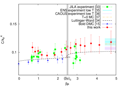
Figure 7: The contact density $\mathcal{C}/\varepsilon_{\rm F}^{2}=\mathcal{C}/k_{\rm F}^{4}$ in the continuum limit versus $\beta\mu$. We compare our results (red circles; the empty circle denotes our result at $T_{c}$ from Goulko and Wingate (2010b)) with experimental data Sagi et al. (2012) (green squares), as well as results obtained with bold DMC Van Houcke et al. (2013) (blue triangles), Luttinger-Ward formalism Enss et al. (2011) (black dashed line) and the zero-temperature results from Navon et al. (2010) (cyan line with error margin), Hoinka et al. (2013) (purple dotted line with error margin) and Gandolfi et al. (2011) (orange dash-dotted line with error margin).

Figure 7 shows the contact density in the continuum limit. There has been recent progress experimentally investigating Tan’s contact, mostly for trapped systems Hoinka et al. (2013); Kuhnle et al. (2011); Stewart et al. (2010) as well as numerical and analytical calculations Van Houcke et al. (2013); Boettcher et al. (2013); Enss et al. (2011); Hu et al. (2011); Palestini et al. (2010); Drut et al. (2011). The homogeneous contact in the normal phase has been studied experimentally in Ref. Sagi et al. (2012). They find a sharp decrease in the contact around the superfluid phase transition. We do not observe any such sudden change around $T_{c}$, but our results above $T_{c}$ show good agreement with their data. Our results at low temperature also show excellent agreement with the zero-temperature numerical Gandolfi et al. (2011) and experimental results Hoinka et al. (2013); Navon et al. (2010) (the contact is not discussed explicitly in the latter reference, but can be easily extracted with the appropriate Tan relation yielding $\mathcal{C}/\varepsilon_{\rm F}^{2}=2\zeta/5\pi=0.1184(64)$).

V Summary and Conclusion

In summary, we have calculated the chemical potential, the energy density and the contact of a homogeneous 3d balanced unitary Fermi gas at different temperatures above and below the critical point. Our results show good agreement with experimental measurements and provide a benchmark for future studies, in particular below $T_{c}$ where few accurate predictions and measurements are available.