Observational evidence for travelling wave modes bearing distance proportional shifts

Abstract

Discrepancies of range between the Space Surveillance Network radars and the Deep Space Network in tracking the 1998 earth flyby of NEAR, and between ESA’s Doppler and range data in Rosetta’s 2009 flyby, reveal a consistent excess delay, or lag, equal to instantaneous one-way travel time in the telemetry signals. These lags readily explain all details of the flyby anomaly, and are shown to be symptoms of chirp d’Alembertian travelling wave solutions, relating to traditional sinusoidal waves by a rotation of the spectral decomposition due to the clock acceleration caused by the Doppler rates during the flybys. The lags thus relate to special relativity, but yield distance proportional shifts like those of cosmology at short range.

The fourth-power power law limits direct radar tracking, as provided by the Space Surveillance Network (SSN), to about the range of geostationary orbits ($36,000~{}\mathrm{k}\mathrm{m}$). For tracking spacecraft on deep space missions, NASA’s Deep Space Network (DSN) uses the telemetry signal returned by the phase-coherent onboard transponder for both range and Doppler measurements, using modulated range codes and the carrier, respectively, as detailed in [1, §III]. Using spin-stabilized spacecraft, this approach achieves sufficient precision for tests of general relativity [2, 3, 4]. Over decades, this approach has led to four space anomalies [5], of which the best known, the Pioneer anomaly, has now been traced to an overlooked radiation reaction [6].

The present work fully explains the earth flyby anomaly, without assuming dark matter (cf. [7]), or modifications to gravitation theory (cf. [8, 9]). A broader result is a local mechanism that relates more closely to special relativity and propagation, yet yields distance proportional spectral shifts along with time dilations, which are thought to need an expanding space-time (cf. [10, 11, 12, 13]).

The distance proportionality is given by large negative residuals of the SSN data [14], against the DSN-estimated trajectory, which, barring contrived hypotheses, can only mean either that the SSN radar echoes were superluminal specially during the flybys, or that the DSN Doppler and range data had an excess delay. These residuals have been omitted in later discussions [15, 9, 16, 17, 18, 19, 20, 21, 22, 23], as they exceed the SSN resolutions, but radar cannot have less than two-way delay or large variations regardless of processing errors.

The excess delay equals light time for the instantaneous range, and the residuals match the radial distance that the spacecraft would travel in that time. Corresponding shifts in the telemetry spectra are implied by the consistency of the demodulated range codes with the delay in the carrier affecting the DSN Doppler. Both effects are traced to large radial Doppler rates not seen with orbiting satellites; their general absence beyond orbit range is also explained below by the spectral selection in the receiving process.

The core contribution, with the broadest significance, is the explanation of the delays and the shifts themselves as properties of travelling wave chirp spectra, since they are impossible from traditional sinusoidal spectra. The chirps relate to sinusoidal wave spectra as rotations over the local frequency-time planes at the source and the receiver, the rotated frequency axes signifying phase accelerations, and equivalently clock accelerations. The shifts result due to causality and the finite speed of light, whose manifestation in the rotated view resembles expansion of space.

The result finally reveals, and closes, a fine gap between d’Alembert’s general solutions and Bernoulli’s solution to the vibrating string problem as a series in sinusoidal waves [24, 25], that has been thought complete because of Fourier theory, but makes sinusoidal transport look fundamental and special. The constancy of frequencies is often assumed as sinusoidal wave solutions (cf. [26, §1.3], [27, §10-8]), or obtained as eigenfunctions of time invariant Hamiltonians (cf. [27, §10-3,4], [28, §28,29]). However, the stationarity of source dynamics or constancy of carrier frequencies has no bearing on decomposition at a receiver, which is strictly computational and dictates the spectral components seen, and thus also lags in time varying component properties, including frequency and wavelength in chirps, which must be travel invariant to satisfy d’Alembert’s equation.

The shifts then arise as chirp lags, but empirical proofs were needed for both the computational choice and reality of the lags, since the distance information is impossible per current theory. The computational aspect and availability of distance information in waves are specifically proved by the absence of the anomaly in the ESA Doppler analysis, which uses a Fourier transform [29], in the Rosetta 2009 flyby [30], while its presence in range data from the same signal, demodulated using a carrier reconstructed with the Doppler rate, required a false ephemeris correction [31].

The SSN range residuals in the 1998 NEAR flyby and the ephemeris discrepancy in the Rosetta 2009 flyby thus bear a fundamental significance complementing relativity, of distinguishing a spectral reference frame from physical space-time. The distinction decouples the wavelengths of reception or observation from the source spectrum, since the received spectrum can be arbitrarily shifted by suitable choice of chirp frequency rates for any source distance, so that tera-hertz or X-ray images can now be obtained under visible illumination, for example. In communication, the capacity of a channel is similarly defined by the sinusoidal assumption [32], but signals of arbitrary wavelengths could be received simultaneously as chirp modes, by using shifts to place them in the transmission band of the same optical fibre, whose capacity would be then unlimited [33, 34].

The SSN residuals and their implication of excess delay in DSN and ESA data, are explained in the next section. The theory of chirp travelling wave spectra is given next, followed by quantitative analyses of the SSN residuals and the flyby anomaly, substantiating the above.

1 Indication of the excess delay in DSN data

To an observer using an accelerating clock, a sinusoidal wave should appear as a chirp having the reverse rate of change of frequency, and chirps with the same frequency rate, as sinusoids. Chirps waves necessarily exhibit frequency lags that yield range in continuous wave frequency modulated (CW-FM) radars. In the accelerated clock view, the chirp lags would appear as frequency shifts which are impossible in sinusoidal waves, and the shifts would be proportional to travel, inconsistent with wave propagation as currently known. Fig. 1 is the graph of the SSN residuals reproduced from [14], with scales of distance and one-way travel times for light overlaid to expose their distance proportionality.

The $900~{}\mathrm{m}$ residual at the start of tracking by the SSN is exactly the range error that would occur in about $131~{}\mathrm{m}\mathrm{s}$, representing an optical path length of $33,000~{}\mathrm{k}\mathrm{m}$, at the radial speed of $6.870~{}\mathrm{k}\mathrm{m}~{}\reciprocal{\mathrm{s}}$, and it far exceeds the known resolutions of $15$-$25~{}\mathrm{m}$ at Altair and $5~{}\mathrm{m}$ at Millstone SSN stations. The negative sign is from the original graph and can only mean that the NEAR spacecraft was that much closer, according to SSN radars, than estimated by DSN.

The delays are also too large to blame radar processing. Coherent radars perform phase correlated integration only to extract weak echoes over noise. The radar use of echoes for round trip timing eliminates ambiguities of modulated range codes, which get repeated and are periodic, but are the source of DSN and ESA range data. The SSN datasets thus denote true round trip times, and large errors solely during flybys would be in any case unlikely. Occam’s razor dictates, given the negative sign, that the DSN signal had an excess delay impossible by current ideas, but consistent with chirping due to acceleration, as follows.

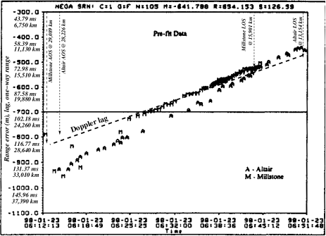
Figure 1: SSN residuals from [14] with lag, range annotations

Denoting the instantaneous range errors as $\Delta r$, and the radial speed as $v_{o}$, the lag times in the figure are given by $\Delta t=\Delta r/v_{o}$, and the one-way ranges, by $r=c\,\Delta t-r_{e}\approx c\,\Delta r/v_{o}-r_{e}$, where $r_{e}\equiv 6.371~{}\mathrm{k}\mathrm{m}$, the earth’s radius. The slope of the residuals thus signifies proportionality of the range error to travel time as $\Delta r=v\Delta t$. The consistency of the DSN Doppler and differenced range data [14, 9] implies the same error affected the DSN Doppler.

The nonrelativistic two-way Doppler is given by $\Delta\nu=2\nu v/c$ at frequency $\nu$ for a velocity $v\equiv dr/dt$, so the DSN phase counters yielded smaller shifts $\Delta\nu^{\prime}=2\nu v^{\prime}/c<\Delta\nu$. The observed travel time proportionality more specifically implies velocity error $d(\Delta r)/dt\equiv\Delta v=d(v\Delta t)/dt\equiv a\Delta t$, where $a$ is the approach acceleration. A Doppler lag can be only significant during a Doppler rate $d(\Delta\nu)/dt=2\nu a/c$, whose lag $d(\Delta\nu)/dt\times\Delta t$ would be therefore of frequency.

The uplink frequency was ramped to keep the downlink steady during the flyby [31], so the delay and lags occurred in the uplink, and were carried into the downlink by the phase-synchronous transponders onboard (cf. [1, §III-A]).

The DSN carrier loop is designed to track the downlink carrier frequency continuously even when its Doppler shift is changing (cf. [35] [1, §III]), hence the DSN phase counts are of cycles of changing periods, whereas Doppler theory was formulated for change in sinusoidal wave periods [36]. The ESA extracts the Doppler using a Fourier transform [29], and thereby conforms to the sinusoidal definition even during accelerations, since each output “bin” of a Fourier transform is a count of cycles around a single frequency. The bound of $4~{}\mathrm{\SIUnitSymbolMicro}\mathrm{m}~{}\reciprocal{\mathrm{s}}\pm 44~{}\mathrm{\SIUnitSymbolMicro}\mathrm{m}~{}\reciprocal{\mathrm{s}}(1\sigma)$ stated against the anomaly in Rosetta’s 2009 flyby [30] are just the resolution and phase noise in the ESA’s Fourier transform.

The reconstructed carrier used for demodulation had to have been again a chirp, however, given the Doppler rate. As Rosetta approached the earth along its orbital motion from behind for gravitational boost (see [37] for all three flyby trajectory diagrams), the earth would have receded over the excess delay in the range data. The $13.34~{}\mathrm{k}\mathrm{m}~{}\reciprocal{\mathrm{s}}$ perigee velocity and $2483~{}\mathrm{k}\mathrm{m}$ altitude suggest $8~{}\mathrm{m}\mathrm{s}$ excess delay, and $110.5~{}\mathrm{m}$ range error as the magnitude of ESA’s erroneous ephemeris correction.

In CW-FM radar, the frequency lags yielding the range comprise cumulative change of transmitter frequency over the radar pulse round trips. Although the Doppler change was similarly continuous in both pre- and post-encounter tracking segments, and the modulated range codes yielded similar lags, the reception process represents a maximum integration time $T$ shorter than a single bit in a modulated range code, so the implied lags and frequency rate of the modulation side-band spectrum, cannot have depended on integration through the round trip. That is, lags in a chirp spectrum depend only on the instantaneous rate, and not a cumulative change of frequency, unlike cosmological shifts.

The residuals are thus evidence for chirp spectra bearing lags exceeding the total carrier variation over the receiver integration times $T$, and for realizability of fractional lags $z\equiv\Delta\nu/\nu\approx\beta r/c\gg\beta T$, variation of the receiver local oscillator (LO), which followed the Doppler rate.

2 Chirp travelling wave spectra

The general form of d’Alembertian solutions $f(r\pm ct)$ requires $f$ invariant of the retarded time $(t-r/c)$. Invariance in $t$ or $r$ separately, generally assumed for separating space and time parts of dynamical equations, would be redundant for waves as the d’Alembertian solutions are already most general. Rather, as characteristic solutions defined by and for the constraint of constant frequencies, sinusoidal waves were never most general. The assumption of constancy avoided a problem, however, that any variation of frequencies with distance $r$ or time $t$ would make the received waves differ from those observable at the source, i.e., at $t=r=0$.

Yet, any travel-invariant property $\xi$ of a travelling wave, hence other than amplitude or phase, should be allowed to vary over time locally at points on the wave path, and must then exhibit the lags $\Delta\xi\equiv\xi(t)-\xi(t-r/c)=\xi(t)-\dot{\xi}r/c+\ddot{\xi}(r/c)^{2}/2!-\ldots\equiv\xi(t)[1-\beta r/c+\beta^{(1)}(r/c)^{2}/2!-\ldots]$, where $\beta\equiv\xi^{-1}d\xi/dt$, $\beta^{(1)}\equiv\xi^{-1}d^{2}\xi/dt^{2}$, $\beta^{(2)}\equiv\xi^{-1}d^{3}\xi/dt^{3}$ …, are fractional derivatives of $\xi$ by the receiver’s clock. This is unlike the Hubble shifts, which are characterized using proper time along the path in current theory.

Fig. 2 shows that such lags must occur in the wavelength of a chirp wave because its local value around each crest and trough moves with the wave. The lag $\Delta\lambda\equiv(\lambda_{4}-\lambda_{1})$ at time $t_{2}$ at receiver $R$ must occur, in a locally measurable sense explained ahead, as the waveform stays unchanged by travel. The fractional shifts $z\approx 1-\beta r/c$ additionally imply time dilations, via the Fourier inverse

$$\int_{\Omega}F(\omega[1+z])\,e^{i\omega t}\,d\omega=\frac{1}{1+z}\,f\left(\frac{t}{1+z}\right),$$ (1)

the amplitude factor denoting stretching of the energy over a dilated interval. Equation (1) governs all uniform shifts, including both Hubble shifts and Doppler, as highlighted recently by the Cassini-Huygens link failure as the signal dilation was overlooked [38]. Dilations were not considered in Dirichlet’s conditions, which assured the completeness of Fourier theory [24, 25]. As a receiver’s local oscillators can be independently varied at arbitrary fractional rates $\beta$, and would yield the corresponding chirp spectra as proved ahead, the reconstructed waveforms would differ from the arriving waves by arbitrary time dilations, which further depend on the distances of the individual sources!

Figure 2: Lags in chirp waves

As a prediction in a differential form from radar imaging [33, 34], this had made no sense and seemed causally flawed [39]. It is finally explained by the computational character of a chirp spectrum in Fig. 3, as a rotation of the receiver’s local frequency ($RR_{\Omega}$) and time ($-RR_{T}$) axes, denoting the local evolution of the spectral components in time by the receiver’s clock. The constant frequency of a sinusoidal component would be represented by vertical lines like $BC$. The inclined lines $GC$, $HF$ denote chirp components with frequencies increasing over time. The spectrum at present time $t_{2}$ is represented by the same coefficient values on the frequency axis $RR_{\Omega}$ regardless of the inclination.

With the inclination, however, excess one-way delays are incurred, just as in the DSN Doppler, that result in shifts exactly equal to cumulative change from an earlier state at the source, so the distance information bears the penalty of excess delay. Each chirp line, projected indefinitely, not only attains every possible frequency at some instant, but is identical to every other chirp of the same inclination by a simple displacement in time. This equivalence leads to the excess delay, as the travel delay acts against the frequency change. Conversely, were the angle of inclination $\angle CBF\equiv\tan^{-1}(|CF|/|BC|)=\tan^{-1}(\beta\Delta t/\Delta t)=\tan^{-1}\beta$ made $0$, the chirps would become degenerate vertical lines through $C$ and $F$ that overlap no longer if displaced in time, so the delay and the distance information both vanish.

These details, and relations to causality and the speed of light, are revealed by incorporating the source frequency ($SS_{\Omega}$) and time ($-SS_{T}$) axes, with corresponding source chirp lines $JD$ and $AE$ parallel to $GC$ and $HF$. Sinusoidal transport would be represented by parallel lines like $DC$ and $EF$ connecting equal values on the source and receiver frequency axes. Hubble’s law would require inclined lines like $EC$ to produce shifts $\Delta\omega=\omega_{4}-\omega_{1}=|CF|$ at distance $r$ and $\Delta\omega_{1}\equiv|LM|\approx|CF|r_{1}/r$ at distance $r_{1}\equiv|EM|$.

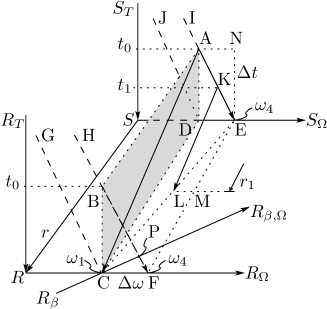
Figure 3: Spatial relation of spectral histories

The $r-ct$ invariance required of d’Alembertian solutions more particularly requires lines like $AC$ and $KL$ inclined at $\angle DAC=\tan^{-1}(|DC|/|AD|)=\tan^{-1}(r/\Delta t)\equiv\tan^{-1}c$ with respect to the time axes, but parallel to the distance vector $SR$, so as to connect equal component frequencies of the source current and receiver voltage spectra, regardless of whether the connected frequencies belong to chirps, as denoted by lines $IE$ and $HF$, or to sinusoids, represented by lines $AD$ and $BC$, respectively. The inclination denotes wave speeds $c<\infty$, and is along of increasing time from source ($A$) to receiver ($C$), conforming to causality.

More importantly, a component with angular frequency $\omega_{1}$ at $C$ on chirp line $GC$ should correspond to the same angular frequency $\omega_{1}$ in source history ($A$), but belong on chirp line $IE$ that changes to $\omega_{4}$ by time $t_{2}$ ($E$). However, an atom emitting at angular frequency $\omega_{4}$ at $t_{2}$ ($E$) would have been observed locally at $\omega_{4}$ also at $t_{0}$ ($N$), and the same should hold for a steady carrier transmission. It thus appears that the d’Alembertian travel lines like $AC$ either require amplitudes to shift with travel, from $N$ to $C$, which would conflict with the d’Alembertian invariance; or chirp spectral decompositions, which can only produce inclined histories like $HF$ and $AE$, must be impossible, so the lags $\Delta\omega$ would require nonlocal simultaneous measurements at source and receiver at $t_{2}$. The second case is cannot hold since the inclinations $\beta$ could be infinitesimally small, and the decomposition is in any case purely computational.

The answer is that the construction already implies that at nonzero $\beta$, $\omega_{1}$ is seen only at distances $r=c\,\Delta\omega/\beta$. The amplitude at $C$ comes from $A$, which is precursor to $E$ at $t_{0}$ and to $N$ at $t_{0}-\Delta t$. The chirp spectrum thus reconstructs distributions at the past times $t_{0}-\Delta t\equiv t_{2}-2\Delta t$, where the factor $2$ relates to the excess delay.

Chirp spectra would be thus time invariant like Fourier spectra, but exhibit distance proportional shift factors and dilations with the receiver’s choice of $\beta$ and its derivatives, because the chirp spectra start fully shifted and dilated at the source! The total energy is also clearly unchanged.

The inclined axis $R_{\beta}R_{\beta,\Omega}$, denotes the chirped spectral view, given by the DSN and ESA range data during flybys, in which local chirp histories $GC$ and $HF$ seem normal to the frequency axis, but travel lines $AC$, $KL$ unaccountably seem inclined. The inclination of axis is equivalent to the receiver’s clock acceleration inclining the components; the segment $|PF$ denotes the relative phase accelerations $|PF|$ that are not apparent in the rotated “reference frame”, in which the chirps appear as a Fourier spectrum with shifts $|CP|\approx\Delta\omega$, due to skewing of all travel lines $AC$, $KL$ to longer wavelengths, as if space itself were expanding.

3 Reception and orthogonality

In any frequency modulation scheme, including phase shift keying (PSK) in deep space telemetry [40], can be described by a random variable $\Omega_{m}$ denoting the instantaneous modulation. Both at the DSN receiver and the spacecraft transponder, the carrier loop phase locks imply, upon allowing for frequency variations, the first order product integral condition

$$\begin{split}\int_{T}\exp\left[\frac{i}{\beta}(\omega_{c}+\Omega_{m})e^{\beta^{\prime}(t-r/c)}\right]\exp\left[-\frac{i\omega_{o}}{\beta}e^{\beta t}\right]dt\\ \simeq 2\pi\,\delta\left(\omega_{c}+\left\langle\Omega_{m}\right\rangle-\omega_{o}\right)\delta(\beta^{\prime}-\beta),\end{split}$$ (2)

where $\omega_{c}$ is the carrier; $\omega_{o}$ is the loop voltage-controlled oscillator (VCO) frequency; $\beta$ and $\beta^{\prime}$ are fractional rates of the VCO and a received spectral component, respectively; and $T$ is the loop filter time constant. $T$ is set below $1~{}\mathrm{Hz}$ in DSN carrier loops in order to suppress both phase noise and modulation [35]. The $\beta^{-1}$ factor is from integrating the exponential chirp $\omega(t)=\omega_{0}e^{\beta t}$ for get the phase, and vanishes in the phase derivative via L’Hôpital’s rule.

Equation (2) constitutes the orthogonality condition for exponential chirp waves without modulation ($\Omega_{m}=0$), and including the case of $T\rightarrow\infty$, since a travelling wave of the same instantaneous frequency and rate of change as the receiver’s LO ($\sim\omega_{o}$) contributes in every cycle to the integration performed by subsequent filters, but any other component contributes over at most a cycle. In a Fourier transform, nonmatching components contribute at every few cycles indefinitely, so Fourier convergence depends on Cesàro means, and is weaker in this sense.

The orthogonality looks weak for distinguishing between say, a chirp of fractional rate $1~{}\reciprocal{\mathrm{s}}$ at $5~{}\mathrm{T}\mathrm{Hz}$ from a $5~{}\mathrm{T}\mathrm{Hz}$ sinusoid as their phases would differ by only $10^{-7}~{}\mathrm{rad}$ over $10^{5}$ cycles, but in a spectral selection or decomposition, all families of curves over local frequency-time planes (Fig. 3) must be assumed available. The contributions from $\beta\pm\delta\beta$ pairs then cancel out for $\delta\beta\neq 0$, just as in the interference of alternative paths in Fermat’s principle. For decoding or demodulation, equation (2) relates the modulated carrier and LO statistically over shorter integration times $T$ for the modulation bandwidth, assuming $\left\langle\Omega_{m}\right\rangle=0$, since the d.c.(direct current) is suppressed in deep space telemetry. The consistency of the DSN range data with its Doppler implies that the modulated chirp spectrum had the correct phase offsets $\Omega_{m}$ relative to the chirp carrier.

Larger lags, of $9~{}\mathrm{M}\mathrm{Hz}$ at $1~{}\mathrm{AU}$ for the same acceleration $0.5~{}\mathrm{m}~{}\mathrm{s}^{-2}$ as at loss of signal (LOS), would shift the chirps out of the filter pass-bands, so the signal presumably gets demodulated from the Fourier spectrum without lags.

4 Explanation of the SSN residuals

The net gain in speed was only $(6.87-6.83)/6.87\approx 0.6\%$ [9, Fig. 3a], with most of the acceleration close to earth after the SSN tracking in increasingly tangential motion. The uniformity of the $10~{}\mathrm{min}$ ticks in the equatorial view [9, Fig. 1] and of similar ticks in the north polar view [14, Fig. 9], which are expanded due to projection, suggest that the mean speed $v_{o}\equiv 6.85~{}\mathrm{k}\mathrm{m}~{}\reciprocal{\mathrm{s}}$ would be adequate for present purposes.

The $219~{}\mathrm{min}$ gap in the DSN tracking then represents $6.851~{}\mathrm{k}\mathrm{m}~{}\reciprocal{\mathrm{s}}\times 219~{}\mathrm{min}=90,000~{}\mathrm{k}\mathrm{m}$ of trajectory. LOS occurred $1\mathrm{h}~{}8\mathrm{min}$ before periapsis and acquisition of signal (AOS), at Canberra, at $2\mathrm{h}~{}31\mathrm{min}$ after periapsis, so the range was $90,000~{}\mathrm{k}\mathrm{m}\times 68/219\approx 27,950~{}\mathrm{k}\mathrm{m}$ at LOS and $62,070~{}\mathrm{k}\mathrm{m}$ at AOS. Tracking at Altair ended $36~{}\mathrm{min}$ past LOS at 06:51:08 and had started at 06:14:28, for a total of $2200~{}\mathrm{s}$, so the tracking started $4120~{}\mathrm{s}$ before periapsis, at $r\approx 4120\times 6.851~{}\mathrm{k}\mathrm{m}~{}\reciprocal{\mathrm{s}}=28,226~{}\mathrm{k}\mathrm{m}$. The one-way delay was therefore $\Delta t\equiv-r/c\approx-94~{}\mathrm{m}\mathrm{s}$, implying range error $\epsilon_{r}\equiv v\,\Delta t=-94~{}\mathrm{m}\mathrm{s}\times 6.851~{}\mathrm{k}\mathrm{m}~{}\reciprocal{\mathrm{s}}\approx-645~{}\mathrm{m}$, about $25\%$ smaller than in Fig. 1. The error decreased with the range rate at $d\epsilon_{r}/dt\approx v\,d(\Delta t)/dt=v^{2}/c=(6.851~{}\mathrm{k}\mathrm{m}~{}\reciprocal{\mathrm{s}})^{2}/c\approx 0.313~{}\mathrm{m}~{}\reciprocal{\mathrm{s}}$, over $1187~{}\mathrm{s}$ from 06:25:25 to 06:45:12, hence by $0.313\times 1187\approx 186~{}\mathrm{m}$, which is within $10\%$ of the $200~{}\mathrm{m}$ Millstone decrease. Fig. 1 shows two sets of residuals, since they are projections of the same lag of the (pre-LOS based) DSN estimate behind the true trajectory in the direction of each of the two SSN stations. The ground track diagram [14, Fig. 7] shows the trajectory pointed towards Millstone initially, implying a faster initial decrease of range, hence greater initial values for Millstone, as seen in Fig. 1.

5 Explanation of the flyby anomaly

The delay means that DSN underestimates pre-encounter approach speed and overestimates post-encounter recession and thus infers an anomalous velocity gain in earth flybys whenever the tracking is discontinuous across periapsis. If tracked continuously, however, the delay in the Doppler’s change of sign at periapsis (Fig. 4) should cause a negative $\Delta v$.

The negative $\Delta v$ in Galileo’s second flyby was concluded from around periapsis, since it was at first thought masked by atmospheric drag [14, 9]. The tracking was unbroken in Cassini’s flyby that also showed negative $\Delta v$ [41].

As the excess delay varies with range, the true velocity profile, given by the differenced SSN range, and the DSN Doppler would be closest at periapsis, and cannot really be parallel. The slopes of the residuals were thus “irreducible through velocity estimation” [14], though both curves were monotonic over the SSN tracking period, as shown.

Figure 4: DSN Doppler and its lags during flybys

The velocity error at AOS should cause post-encounter data to be inconsistent with the pre-encounter trajectory, and vice versa. Acceleration due to earth’s gravity at AOS range would be $a=0.103~{}\mathrm{m}~{}\mathrm{s}^{-2}$, implying a velocity error $\Delta v=-a\Delta t\approx 21.4~{}\mathrm{m}\mathrm{m}~{}\reciprocal{\mathrm{s}}$, or a $603~{}\mathrm{m}\mathrm{Hz}\sim 10.7~{}\mathrm{m}\mathrm{m}~{}\reciprocal{\mathrm{s}}$ Doppler amplitude at the downlink frequency. These are about $20\%$ of the reported $760~{}\mathrm{m}\mathrm{Hz}=13.5~{}\mathrm{m}\mathrm{m}~{}\reciprocal{\mathrm{s}}$ [9].

Canberra’s latitude of $35.2828\mathrm{\SIUnitSymbolDegree}$ means it is $6371~{}\mathrm{k}\mathrm{m}\times\cos(35.2828\mathrm{\SIUnitSymbolDegree})=5201~{}\mathrm{k}\mathrm{m}$ off the earth’s axis. The $-71.96\mathrm{\SIUnitSymbolDegree}$ declination of the post-encounter velocity asymptote then implies $5201~{}\mathrm{k}\mathrm{m}\times\cos(71.96\mathrm{\SIUnitSymbolDegree})\approx 1611~{}\mathrm{k}\mathrm{m}$ of diurnal range and $(1611/62070)\times 603~{}\mathrm{m}\mathrm{Hz}\approx 15.6~{}\mathrm{m}\mathrm{Hz}$ diurnal Doppler oscillations. The larger actual $50~{}\mathrm{m}\mathrm{Hz}$ amplitude is due to a smaller declination at AOS, and to a misprediction of direction [9], possibly worsened by the error at LOS.

The velocity error $\Delta v=-a\Delta t\equiv-ar/c$ also explains the $r^{-1}$ decay in the post-encounter oscillation graphs [14, 9], since $a\propto r^{-2}$ due to earth’s gravity.

6 Conclusion

All features of the flyby anomaly are thus explained by a delay proportional to range in Doppler and range data derived from the telemetry signal that was chirped due to the Doppler rate, and should be impossible by current notions of wave propagation.

More particularly, the distance proportionality of the delay and of the equivalent frequency lags in the telemetry spectrum are given by two independent radar tracks which had been overlooked for over a decade, oddly, in the very quest for deviations from the known laws.

The chirping and lags should be also easy to verify over ground distances at radio frequencies, with no motion or the difficulties of optical implementation (cf. [34]).

References

- [1] J D Anderson, P A Laing, E L Lau, A S Liu, M Nieto, and S G Turyshev. Study of the anomalous acceleration of Pioneer 10 and 11. Phys Rev D, 65:082004/1–50, Apr 2002. Report LA-UR-00-5654, arXiv:gr-qc/0104064.
- [2] P L Bender and M A Vincent. Small Mercury Relativity Orbiter. Technical Report N90-19940 12-90, NASA, Aug 1989.
- [3] M A Vincent and P L Bender. Orbit determination and gravitational field accuracy for a Mercury transponder satellite. J Geophy Res, 95:21357–21361, Dec 1990.
- [4] J D Anderson et al. Gravitational wave background in coincidence experiments with Doppler tracking of interplanetary spacecraft. Am Astro Soc Meeting, 182(05.11), May 1993.
- [5] J D Anderson and M M Nieto. Astrometric solar-system anomalies. Aug 2009. arXiv:gr-qc/0907.2469v2.
- [6] S G Turyshev, V T Toth, G Kinsella, S C Lee, S M Lok, and J Ellis. Support for the thermal origin of the Pioneer anomaly. Phys Rev Lett, 108, 2012. arXiv:1204.2507v1.
- [7] S L Adler. Modeling the flyby anomalies with dark matter scattering: update with additional data and further predictions. Int J Mod Phys A, 28, Dec 2011. arXiv:1112.5426.
- [8] J D Anderson et al. Indication from Pioneer 10/11, Galileo and Ulysses data of an apparent anomalous, weak, long-range acceleration. Phys Rev Lett, 81:2858–2861, Oct 1998. arXiv:gr-qc/9808081.
- [9] J D Anderson, J K Campbell, J E Ekelund, J Ellis, and J F Jordan. Anomalous orbital-energy changes observed during spacecraft flybys of earth. PRL, 100(9):091102, 2008.
- [10] A Sandage and L M Lubin. The Tolman Surface Brightness Test for the Reality of the Expansion. I-IV. Astro J, 121:2271-300, 122:1071-1103, 2001. arXiv:astro-ph/0102213.
- [11] E Wolf. Noncosmological redshifts of spectral lines. Nature, 326:363–365, 1987.
- [12] E Wolf. Redshifts and blueshifs of spectral lines caused by source correlations. Opt Comm, 62:12–16, 1987.
- [13] E Wolf et al. Frequency shifts of spectral lines … J Opt Soc Am A, 6(8), Aug 1989.
- [14] P G Antreasian and J R Guinn. Investigations into the unexpected Delta-V increases during the earth gravity assists of Galileo and NEAR. AIAA, 1998. 98-4287.
- [15] J D Anderson, J K Campbell, and M M Nieto. The Energy Transfer Process in Planetary Flybys. NewAstron, 12:383–397, Nov 2006. arXiv.org:astro-ph/0608087v2.
- [16] M B Gerrard and T J Sumner. Earth flyby and pioneer anomalies. Oct 2008. arXiv:gr-qc/0807.3158v2.
- [17] J P Mbelek. Special relativity may account for spacecraft flyby anomalies. Mar 2009. arXiv:0809.1888v3.
- [18] M E McCulloch. Modelling the flyby anomalies using a modification of inertia. MNRAS Lett, 389(1):L57–L60, 2008. arXiv:0806.4159.
- [19] S G Turyshev and V T Toth. The Puzzle of the Flyby Anomaly. Space Sci Rev, 148:169–174, 2010. arXiv:gr-qc/0907.4184v1.
- [20] G G Nyambuya. Are Flyby Anomalies and the Pioneer Effect an ASTG Phenomenon? May 2010. arXiv:0803.1370v4.
- [21] O Bertolami, F Francisco, P J S Gil, and J Páramos. Probing the Flyby Anomaly with the Galileo Constellation. Sep 2011. arXiv:1109.2779.
- [22] J Páramos and G Hechenblaikner. Probing the Flyby Anomaly with the future STE-QUEST mission. Oct 2012. arXiv:1210.7333.
- [23] L Lorio. A flyby anomaly for Juno? Not from standard physics. Nov 2013. arXiv:1311.4218.
- [24] I Kleiner. Evolution of the function concept: A brief survey. The College Math J, 20(4):282–300, 1989.
- [25] G F Wheeler and W P Crummett. The vibrating string controversy. Am J Phys, 55(1):33–37, 1987.
- [26] M Born and E Wolf. Principles of optics: Electromagnetic theory of propagation, interference and diffraction of light. Cambridge University Press, 7th edition, 2002.
- [27] H Goldstein. Classical Mechanics. Addison-Wesley, 2nd edition, 1980.
- [28] P A M Dirac. The Principles of Quantum Mechanics. Cambridge Univ, 4th edition, 1953.
- [29] B E Jensen. New high performance integrated receiver/ranging/demodulator system for ESTRACK. 1998.
- [30] T Morley. http://webservices.esa.int/blog/post/5/916. https://web.archive.org/web/20120327190538/, 2009.
- [31] P G Antreasian and W Folkner. Pvt comm, 2015.
- [32] C E Shannon. Communication in the presence of noise. Proc IRE, 37(1):10–21, 1949. Reprint: Proc IEEE Feb 1998.
- [33] V Guruprasad. A wave effect enabling universal frequency scaling, monostatic passive radar, incoherent aperture synthesis, and general immunity to jamming and interference. In MILCOM (classified session), 2005. arXiv:physics/0812.2652v1.
- [34] V Guruprasad. Prediction of spectral shifts proportional to source distances by time-varying frequency or wavelength selection. In Proc. Nature of Light II: Light in Nature, SPIE Optics+Photonics Symp, Aug 2008. Paper no. 7057-11. Also: arXiv:physics/0812.1004v1.
- [35] D K Shin. 202, Rev. B 34-m and 70-m Doppler. In 810-005 DSN Telecommunications Link Design Handbook. Sep 2010.
- [36] J C A Doppler. On the coloured light of the binary stars and other celestial bodies. Prague: K Bohm Gesellschaft der Wissenschaften, 1842. (in German).
- [37] M Billvik. The first Rosetta flyby – trajectory, attitude and radiation information for LAP operations. PhD thesis, Uppsala, 2005. UPTEC F05 063.
- [38] J Oberg. Titan calling. IEEE Spectrum, Oct 2004.
- [39] B G Elmegreen. Pvt comm, 2009.
- [40] R W Sniffin. 208, Rev. A Telemetry Data Decoding. In 810-005 DSN Telecommunications Link Design Handbook. 2009.
- [41] M E Burton, B Buratti, D L Matson, and J P Lebreton. The Cassini/Huygens Venus and Earth flybys: An overview of operations and results. J Geophys Res, 106(A12):30099–30107, 2001.