Geometrical Scaling
in Inelastic Inclusive Particle Production at the LHC

Abstract

Analyzing recent ALICE data on inelastic pp scattering at the LHC energies we show that charged particle distributions exhibit geometrical scaling (GS). We show also that the inelastic cross-section is scaling as well and that in this case the quality of GS is better than for multiplicities. Moreover, exponent $\lambda$ characterizing the saturation scale is for the cross-section scaling compatible with the one found in deep inelastic ep scattering at HERA. Next, by parametrizing charged particles distributions by the Tsallis-like formula, we find a somewhat unexpected solution that still exhibits GS, but differs from the ”standard” one where the Tsallis temperature is proportional to the saturation scale.

I Introduction

It is believed that gluon distribution inside a hadron saturates at small Bjorken $x$ (see Refs. Mueller:2001fv ; McLerran:2010ub for review). This is a consequence of the non-linear QCD evolution equations, known as Balitsky-Kovchegov (BK) equation BK or in a more general case as JIMWLK equation jimwlk , that poses traveling wave solutions Munier:2003vc . The latter property, in the QCD context, is called geometrical scaling (GS) Stasto:2000er . An effective theory relevant for the small Bjorken $x$ region is so called Color Glass Condensate (CGC) MLV . For the purpose of present work the details of the saturation are not of primary importance; it is the very existence of the saturation scale which plays the crucial role

Geometrical scaling means that some observable $N$ that in principle depends on two independent kinematical variables, say $x$ and $Q^{2}$, in fact depends only on a specific combination of them denoted as $\tau$:

$$N(x,Q^{2})={\cal F}(\tau).$$ (1)

Here function ${\cal F}$ in Eq. (1) is a dimensionless function of a scaling variable fn1

$$\tau=Q^{2}/Q_{\rm s}^{2}(x).$$ (2)

and

$$Q_{\rm{s}}^{2}(x)=Q_{0}^{2}\left({x}/{x_{0}}\right)^{-\lambda}$$ (3)

is the saturation scale. The power law form of the saturation scale is dictated by a saddle-point solution to the BK equation and has been tested phenomenologically for different high energy processes Stasto:2000er –Praszalowicz:2013uu .

Here we are coming back to pp scattering McLerran:2010ex in the context of recently published ALICE data Abelev:2013ala for charged particle distributions at three LHC energies 0.9, 2.76 and 7 TeV. After discussing shortly in Sect. II how GS emerges in the $k_{\rm T}$ factorization scheme, we shall show in Sect. III that recent ALICE data indeed exhibit geometrical scaling with, however, $\lambda$ exponent being different than in the case of deep inelastic (DIS) ep scattering. Interestnigly, we shall also show that the inclusive cross-sections scale somewhat better and with an exponent that is very close to the DIS value $\lambda=0.32$ Praszalowicz:2012zh . This result calls for better understanding of the impact parameter picture of pp scattering in the context of the saturation physics and the Color Glass Condensate theory.

Another topic addressed in the present paper is the shape of the scaling function introduced schematically in Eq. (1). Function $\cal{F}$ can be in fact obtained only numerically within some specific model. Here, we shall use phenomenological parametrization in the form of Tsallis-like distribution Tsallis applied successfully in the past to describe spectra of charged particles Wong:2012zr –Cleymans:2013rfq . In Sect.IV we briefly describe how GS should be reflected in the Tsallis distribution. Next, in Sect. V we shall try do fit Tsallis-like parametrization to the ALICE data. Unfortunately, as already remarked in the original ALICE publication Abelev:2013ala , this piece of data does not admit good quality Tsallis fit. Nevertheless, we invoke a procedure that allows for rather good description of the data in the range of moderate transverse momenta where GS is expected to occur. Somewhat unexpectedly we find GS scaling solution that is very different from the ”standard” one described in Sect. IV. Unfortunately GS in this solution is rather accidental and will disappear at very high energies. Whether this is only a property of the Tsallis parametrization ”forced” to describe ALICE data, or a real prediction, remains to bee seen. We conclude in Sect. VI

II Geometrical scaling in hadronic collisions

The cross-section for producing a moderate $p_{\rm{T}}$ gluon in hadronic collision can be described as Gribov:1981kg :

$$\frac{d\sigma}{dyd^{2}p_{\rm T}}=\frac{C}{p_{\rm{T}}^{2}}{\displaystyle\int}d^{2}\vec{k}_{\rm{T}}\,\alpha_{\rm{s}}(k_{\rm{T}}^{2})\varphi_{1}(x_{1},\vec{k}_{\rm{T}}^{2})\varphi_{2}(x_{2},(\vec{k}-\vec{p})_{\rm{T}}^{2})$$ (4)

where $C$ contains color factors and numerical constants. Bjorken $x$’s of colliding partons read

$$x_{1,2}=\frac{p_{\mathrm{T}}}{\sqrt{s}}\,e^{\pm y}$$ (5)

however, since in the following we will be interested in central rapidity production, i.e. $y\simeq 0$, we have $x_{1}\simeq x_{2}=x$. Functions $\varphi_{1,2}$ are the unintegrated gluon distributions in hadron $h_{1}$ and $h_{2}$ respectively. There exist many models of unintegrated gluon distributions (see e.g. Szczurek:2003vq ); the most simple ones are the one of the Golec-Biernat–Wüsthoff (GBW) model  GolecBiernat:1998js or the one by Kharzeev, Levin and Nardi Kharzeev:2002ei . They share two important features: geometrical scaling and dependence on the transverse area $S_{\bot}$ whose precise meaning is best understood in a picture where also the impact parameter is taken into account Kowalski:2003hm ; Tribedy:2010ab . Therfore

$$\varphi(x,\vec{k}_{\rm{T}}^{2})=S_{\bot}\phi(k_{\rm{T}}^{2}/Q_{\rm{s}}^{2}(x))$$ (6)

where $\phi$ is a dimensionless function of the scaling variable $k_{\rm{T}}^{2}/Q_{\rm{s}}^{2}(x)$, rather than independently of $x$ and $k_{\rm{T}}^{2}$. Of course geometrical scaling is only an approximation and is expected to break for large Bjorken $x$’s and also for large transverse momenta. We also expect GS breaking for small $k_{\rm T}$ where non-perturbative effects including effects from the pion mass are of importance. Ignoring these effects and neglecting also momentum dependence of the strong coupling constant we arrive at

$$\frac{d\sigma}{dyd^{2}p_{\rm{T}}}=\frac{S_{\bot}^{2}}{2\pi}\mathcal{F}(\tau)$$ (7)

where $\mathcal{F}$ is a universal, energy independent function of the scaling variable $\tau$:

$$\tau=\frac{p_{\rm{T}}^{2}}{Q_{\rm{s}}^{2}(x)}=\left(\frac{p_{\rm{T}}}{Q_{0}}\right)^{2}\left(\frac{p_{\rm{T}}}{\xi W}\right)^{\lambda}.$$ (8)

Here we have used (3) for the saturation scale $Q_{\mathrm{s}}^{2}$. We take for $x_{0}=\xi\times 10^{-3}.$ This implies that in (8) $p_{\rm{T}}$ is in GeV$/c$ and $W$ in TeV. Furthermore for $Q_{0}$ we can take without any loss of generality $Q_{0}=1$ GeV$/c.$ One typically assumes that $S_{\bot}$ is an energy independent constant. This is true in the case of the GBW model GolecBiernat:1998js where $S_{\bot}=\sigma_{0}$ with $\sigma_{0}$ characterizing the asymptotics of the dipole-proton cross-section for large dipole sizes. In the case of heavy ion collisions for fixed centrality, $S_{\bot}$ has geometrical interpretation as an overlap area of two colliding nuclei Kharzeev:2002ei . In this case one can also assume that

$$\frac{d\sigma}{dyd^{2}p_{\rm{T}}}=S_{\bot}\frac{d^{2}N}{dyd^{2}p_{\rm{T}}}$$ (9)

where $N$ is a multiplicity of produced gluons. Neglecting possible energy dependence of gluon fragmentation into hadrons Levin:2011hr , i.e. adopting parton-hadron duality hypothesis PHD , we arrive at:

$$\frac{1}{p_{\rm{T}}}\frac{d^{2}N_{\rm{ch}}}{dydp_{\rm{T}}}=S_{\bot}\mathcal{F}(\tau).$$ (10)

Expression (10) will be used in the following to look for GS in the multiplicity distributions. Let us, however, note that GS is in fact a property of Eq.(7) and that the multiplicity scaling (10) is based on (9) which is not so obvious for the scattering of small systems, like pp.

In order to integrate (10) over $d^{2}p_{\rm{T}}$ we have to change variables

$$p_{\rm{T}}=\overline{Q}_{\rm{s}}(W)\tau^{1/(2+\lambda)}$$ (11)

where the average saturation scale is defined as

$$\overline{Q}_{\rm{s}}(W)=Q_{0}\left(\frac{\xi W}{Q_{0}}\right)^{\lambda/(2+\lambda)}.$$ (12)

Note that the effective power describing the rise of the average saturation scale with energy $\lambda_{\mathrm{eff}}=\lambda/(2+\lambda)$ is slightly smaller than $\lambda/2$. Then

$$p_{\rm{T}}dp_{\rm{T}}=\frac{1}{2+\lambda}\overline{Q}_{\rm{s}}^{2}(W)\,\tau^{2/(2+\lambda)}\frac{d\tau}{\tau}.$$ (13)

Hence

$$\frac{dN_{\rm ch}}{dy} = \left[\frac{1}{2+\lambda}{\displaystyle\int}\mathcal{F}(\tau)\tau^{2/(2+\lambda)}\frac{d\tau}{\tau}\right]\times S_{\bot}\overline{Q}_{\rm{s}}^{2}(W)$$ (14)

$$= b\times S_{\bot}\overline{Q}_{\rm{s}}^{2}(W)\ .$$

Here $b$ is an energy independent constant related to the the integral of $\mathcal{F}(\tau)$. Equation (14) is often used as a definition of the saturation scale (with $N_{\rm ch}$ replaced by $N_{\rm gluons}$) understood as gluon number density per transverse area.

III Geometrical scaling of ALICE data

In this Section we are going to check whether ALICE data Abelev:2013ala on inelastic multiplicity distributions of charged particles exhibits geometrical scaling and for what value of $\lambda$. We shall show that indeed GS is reached for $\lambda\sim 0.22-0.24$ as it is illustrated in Fig. 1.

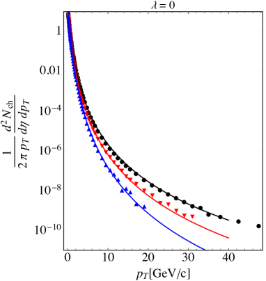
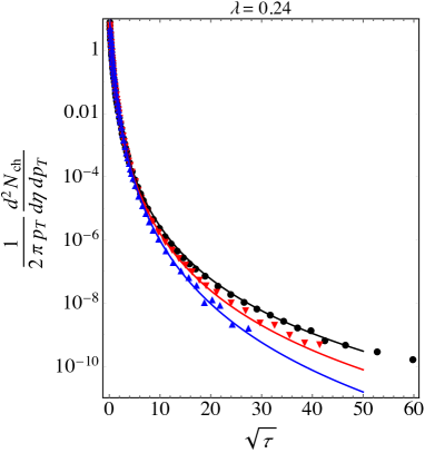
Figure 1: Charged particle spectra measured by ALICE Abelev:2013ala , plotted as functions of $p_{\mathrm{T}}$ (left panel) and as functions of the scaling variable $\tau$ (8) for $\lambda=0.24$ (right panel). Black full dots correspond to $W=7$ TeV, red down-triangles to 2.76 TeV and blue up-triangles to 0.9 TeV. Solid lines correspond to the Tsallis fits from Sect. V.

In order to find the best value of $\lambda$ we have adopted the method of ratios described in more detail in Refs. Praszalowicz:2012zh . Let us denote for simplicity

$$N(p_{\rm{T}},W)=\left.\frac{1}{2\pi p_{\rm{T}}}\frac{d^{2}N_{\rm ch}}{dydp_{\rm{T}}}\right|_{W}.$$ (15)

We form ratios of spectra expressed in terms of the scaling variable $\tau$ rather than in terms of $p_{\mathrm{T}}$:

$$R_{W/W^{\prime}}(\tau)=\frac{N(\tau,W)}{N(\tau,W^{\prime})}$$ (16)

and request that $R\sim 1$ over the largest possible interval of $\tau$. Note that this method is sensitive only to the value of $\lambda$ and not to the actual values of parameters $Q_{0}$ and $x_{0}$ In the present case we choose 7 TeV for $W$ and $W_{1}=2.76$ or $W_{2}=0.9$ TeV for $W^{\prime}$. Therefore we can form two such ratios, which are depicted in Fig. 2 for $\lambda=0$ (i.e. for $\sqrt{\tau}=p_{\mathrm{T}}$) and for $\lambda=0.24$. We see that indeed, these two ratios that rise rather steeply with $p_{\mathrm{T}}$, remain flat and close to 1 if plotted in terms of $\sqrt{\tau}$ for $\lambda=0.24$. We interpret this as a signature of geometrical scaling.

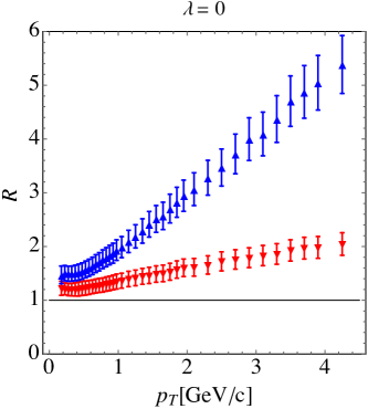
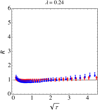
Figure 2: Ratios of charged particle spectra measured by ALICE Abelev:2013ala , plotted as functions of $p_{\mathrm{T}}$ (left panel) and as functions of the scaling variable $\tau$ (8) for $\lambda=0.24$ (right panel). Red down-triangles correspond to to the ratio 7/2.76 TeV and blue up-triangles to 7/0.9 TeV.

In order to decide on the best value of exponent $\lambda$ we need to provide a quantitative criterion measuring the ”average distance” of experimental values of $R_{W/W^{\prime}}$ from unity. To this end we propose the following procedure. Since for $\lambda$ values relevant for the present analysis the first few $R$ points corresponding to low $p_{\mathrm{T}}$ lie above 1 (which is the sign of GS violation in a region when non-perturbative effects are of importance) we pick up the first point for which

$$R_{W/W_{1,2}}(\tau_{\mathrm{start}})-1\leq\Delta_{R}(\tau_{\mathrm{start}}).$$

Here $\Delta_{R}$ is an experimental error of $R$. For points with $\tau>\tau_{\mathrm{start}}$ ratio $R$ is either close to 1 within the experimental errors, or it is falling below 1 exceeding $\Delta_{R}$. Next, since for large transverse momenta $p_{\mathrm{T}}$ spectra are getting harder with increasing energy, the values of $R$ start to increase with $\tau$, getting again larger than 1. This is well visible in Fig. 3 where the vertical scale has been magnified with respect to Fig. 2 for better resolution.

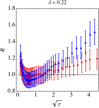
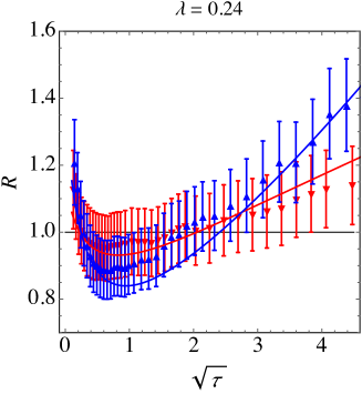
Figure 3: Same as Fig. 2 with different scale for better resolution. Solid lines in the right panel correspond to the Tsallis fits from Sect. V.

Starting from $\tau_{\mathrm{start}}$ that of course depends on energy $W_{1,2}$, we compute mean square deviation for given $\lambda$

$$\delta_{W_{1,2}}^{2}(\lambda)=\frac{1}{n_{W_{1,2}}(\lambda)}{\displaystyle\sum\limits_{\tau_{n}=\tau_{\mathrm{satrt}}}^{\tau_{\mathrm{end}}}}\frac{\left(R(\tau_{n},W_{1,2})-1\right)^{2}}{\Delta_{R}^{2}(\tau_{n},W_{1,2})}$$ (17)

where $n_{W_{1,2}}(\lambda)$ is a number of points between $\tau_{\mathrm{start}}$ and $\tau_{\mathrm{end}}$. We increase $\tau_{\mathrm{end}}$ up to the last point where $\delta_{W_{1,2}}^{2}(\lambda)<1$. In this way we obtain $n_{W^{\prime}}(\lambda)$ which is the number of points that exhibit GS for given $W^{\prime}=W_{1,2}$ and for given $\lambda$, which are plotted in Fig. 4. Now we look for maximum of $n_{W_{1}}(\lambda)+n_{W_{2}}(\lambda)$. This happens for $\lambda=0.24$. As seen from Fig. 3 $W_{2}=0.9$ TeV points scale in a shorter interval of $\tau$, which translated back to transverse momenta corresponds to $p^{\mathrm{max}}_{\mathrm{T}}=3.1$ GeV$/c$. We see from Fig. 3 (right panel) that although $\delta_{W_{2}}^{2}<1$ there are 0.9 TeV points (blue up-triangles) in the region $\tau_{\mathrm{start}}\leq\tau\leq\tau_{\mathrm{end}}$ which are below 1 outside the experimental error. If we demand that all points between $\tau_{\mathrm{start}}$ and $\tau_{\mathrm{end}}$ should be equal to unity within experimental errors, then $\lambda=0.22$. This is the value of $\lambda$ used in Refs. McLerran:2014apa and the relevant plot is shown in the left panel of Fig. 3. The corresponding $p^{\mathrm{max}}_{\mathrm{T}}$ is shifted down to 2.9 GeV$/c$.

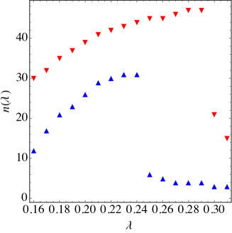
Figure 4: Number of points that contribute to (17) for two different ratios: 7/2.76 TeV (red down-triangles) and 7/0.9 TeV (blue up-triangles) plotted as functions of $\lambda$.

Interestingly, when we repeat this procedure for the cross-sections which are obtained by multiplying the multiplicity spectra by the minimum bias cross-section $\sigma_{\mathrm{MB}}(W)$ given explicitly in Ref. Abelev:2013ala , we find that GS occurs at a higher value of $\lambda=0.31-0.33$. This by itself is not surprising since $\sigma_{\mathrm{MB}}(W)$ depends on energy and this dependence makes $\lambda$ different than in the case of multiplicity. What is, however, surprising and encouraging is that the value of $\lambda$ is now consistent with DIS. Moreover, the range of GS is now larger, up to $p^{\mathrm{max}}_{\mathrm{T}}=4.25$ GeV$/c$. This is depicted in Fig. 5. The explanation of this observation is beyond the scope of the present paper, however, it is clear that it requires a more sophisticated model of $S_{\bot}$ of Eq. (9), which in the present analysis is assumed to be an energy independent constant in the case of multiplicity scaling or minimum bias cross-section in the case of cross-section scaling.

We have performed similar analysis for the UA1 data Albajar:1989an for p$\bar{\mathrm{p}}$ cross-section at $\sqrt{s}=0.2$, 0.5 and 0.9 TeV with similar result that $\lambda\approx 0.34$. Here, however, the data extends only up to $\sim 7$ GeV$/c$ (for two lower energies) and the tail is quite noisy, namely the ratios of the cross-sections fluctuate quite significantly for $\sqrt{\tau}>3$.

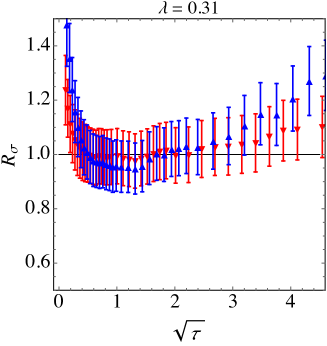
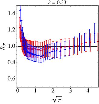
Figure 5: Ratios of charged particle cross-sections measured by ALICE, plotted as functions of the scaling variable $\tau$ (8) for $\lambda=0.31$ (left panel) and for $\lambda=0.33$ (right panel). Red down-triangles correspond to to the ratio 7/2.76 TeV and blue up-triangles to 7/0.9 TeV.

IV Geometrical Scaling and Tsallis parametrization

It is well known that particle spectra at low and medium transverse momenta can be described by thermal distributions in transverse mass $m_{\mathrm{T}}=\sqrt{p_{\mathrm{T}}^{2}+m^{2}}$ with ”temperature” $T$ which is a function of the scattering energy Hagedorn . It is also known that more accurate fits are obtained by means of Tsallis-like parametrization Tsallis where particle multiplicity distribution takes the following form (see e.g. Chatrchyan:2012qb ):

$$\frac{1}{2\pi p_{\rm{T}}}\frac{d^{2}N_{\rm ch}}{dydp_{\rm{T}}}=\frac{dN_{\rm ch}}{dy}\frac{p}{E}\frac{C_{n}}{2\pi}\left[1+\frac{\widetilde{E}_{\rm{T}}}{n\,T}\right]^{-n}$$ (18)

where $\widetilde{E}_{\rm{T}}=\sqrt{m^{2}+p_{\rm{T}}^{2}}-m$. In what follows we shall keep $m=0$ what implies $p/E=1$. Here

$$C_{n}=\frac{(n-1)(n-2)}{n\,^{2}T^{2}}.$$ (19)

Coefficient $C_{n}$ in Eq. (19) ensures proper normalization of (18). Indeed

$$\frac{dN_{\rm ch}}{dy} = \int\frac{1}{2\pi p_{\rm{T}}}\frac{d^{2}N_{\rm ch}}{dydp_{\rm{T}}}d^{2}p_{\rm{T}}$$ (20)

$$= \frac{dN_{\rm ch}}{dy}C_{n}{\displaystyle\int\limits_{0}^{\infty}}dp_{\rm{T}}p_{\rm{T}}\left[1+\frac{p_{\rm{T}}}{n\,T}\right]^{-n}$$

where the last integral is equal $1/C_{n}.$ Here $n$ and $T$ are free fit parameters that depend on particle species and on energy.

In the limit $n\rightarrow\infty$ (or equivalently for small $p_{\rm T}$) distribution (18) tends to the exponent

$$\frac{1}{p_{\rm{T}}}\frac{d^{2}N_{\rm ch}}{dydp_{\rm{T}}}\simeq\frac{dN_{\rm ch}}{dy}\frac{1}{T^{2}}\exp(-p_{\mathrm{T}}/T).$$ (21)

Substituting (11) into (21) we arraive at:

$$\frac{1}{p_{\rm{T}}}\frac{d^{2}N_{\rm ch}}{dydp_{\rm{T}}}\simeq\frac{dN_{\rm ch}}{dy}\frac{1}{T^{2}(W)}\exp\left(-\frac{\overline{Q}_{\rm{s}}(W)}{T(W)}\tau^{1/(2+\lambda)}\right)$$ (22)

Equation (22) exhibits geometrical scaling exactly, only when Praszalowicz:2013fsa

$$T(W)=\frac{1}{\varkappa}\overline{Q}_{\rm{s}}(W).$$ (23)

Then, using Eq. (14), we get:

$$\frac{1}{p_{\rm{T}}}\frac{d^{2}N_{\rm ch}}{dydp_{\rm{T}}}\simeq\frac{b\varkappa^{2}}{Q_{0}^{2}}\exp\left(-\varkappa\,\tau^{1/(2+\lambda)}\right).$$ (24)

Indeed, (24) is energy independent. This would generalize to the full Tsallis distribution if exponent $n$ were constant. We know, however, from the phenomenological fits that $n$ is decreasing with energy making $p_{\rm{T}}$ spectra harder and – in the same time – introducing explicit violation of geometrical scaling for particle spectra.

Let us observe that we can include factor $\xi$ into a definition of $b$ and $\varkappa$, so without any loss of generality we can set $\xi=1.$ Therefore we finally arrive at the GS-Tsallis parametrization of the $p_{\rm{T}}$ spectra that reads:

$$\left.\frac{1}{2\pi p_{\rm{T}}}\frac{d^{2}N_{\rm ch}}{dydp_{\rm{T}}}\right|_{W} = \frac{B}{Q_{0}^{2}}C_{n_{W}}\left[1+\frac{\varkappa\,p_{\rm{T}}}{n_{W}\,\overline{Q}_{\rm{s}}(W)}\right]^{-n_{W}}$$ (25)

where we have introduced new constant $B=b\varkappa^{2}/2\pi$ and explicitly indicated that $n$ is a function of $W$. This dependence would be of course a source of GS violation. Constants $B$, $\varkappa$ and $Q_{0}$ should remain energy independent.

V Tsallis parametrization of ALICE data

In this Section we are going to check whether one can fit ALICE data Abelev:2013ala with the help of formula (25). In the original ALICE paper Abelev:2013ala it is said that the multiplicity data can be fitted with the Hagedorn distribution Hagedorn , rather than with the Tsallis one. Therefore we could expect that ordinary fitting procedures would not give a reasonable parametrization of the data. In order to enforce Tsallis parametrization we have proceeded in the following way. For each LHC energy we have chosen two values of $p_{\rm{T}}$, one in the small $p_{\rm{T}}$ region and one in the tail that are displayed in Table 1. For $p_{\rm{T}}^{\rm{low}}$ we have chosen approximately 0.5 GeV$/c$ that is already above the non-perturbative region. For $p_{\rm{T}}^{\rm{high}}$ we have chosen values that are rather far from the end of the spectrum, but already large enough to be in the perturbaitve regime. Of course our fit parameters do depend on this choice, however, as we shall see below, the quality of the Tsallis fits with the values of limiting $p_{\rm T}$ given in Table 1 is good enough that manipulating with these values has not been necessary. Let us also remark at this point that our aim here was to show certain properties of the Tsallis fits enforced on ALICE data at low and moderate transverse momenta, since we new from the beginning that this particular piece of data does not admit Tsallis parametrization in the whole $p_{\rm T}$ range.

$W\,$[TeV]	$p_{\rm{T}}^{\rm{low}}$ [GeV$/c$]	$p_{\rm{T}}^{\rm{high}}$ [GeV$/c$]
0.90	0.525	8.5
2.76	0.525	10.5
7.00	0.525	13.5

Table 1: Values of $p_{\rm{T}}^{\rm{low}}$ and $p_{\rm{T}}^{\rm{high}}$ used to fit Tsallis parametrization to ALICE data (see the beginning of Sect. V).

For the $p_{\rm{T}}$ values given in Table 1 we have calculated ratios $N(p_{\rm{T}}^{\rm{low}},W)/N(p_{\rm{T}}^{\rm{high}},W)$, both for the data and for parametrization (25). In this way normalization parameter $B$ canceled out. Now, for fixed value of $\varkappa$ we have calculated $n_{W}$ from the following condition:

$$\varkappa:\;\left.\frac{N(p_{\rm{T}}^{\rm{low}},W)}{N(p_{\rm{T}}^{\rm{high}},W)}\right|_{\rm{th}}=\left.\frac{N(p_{\rm{T}}^{\rm{low}},W)}{N(p_{\rm{T}}^{\rm{high}},W)}\right|_{\rm{exp}}\;\Rightarrow\;n_{W}.$$ (26)

Note that the value of parameter $\lambda$ entering the definition of the saturation scale (12) has been already fixed by the method desribed in Sect. III. Here we have used $\lambda=0.24$.

Next, for each pair $(\varkappa,n_{W})$ we have computed mean quadratic deviation

$$\sigma_{W}^{2}(\varkappa)=\frac{1}{i^{W}_{\rm{max}}}{\displaystyle\sum\limits_{i=1}^{i^{W}_{\rm{max}}}}\frac{\left(\left.N(p_{\rm{T}}^{i},W)\right|_{\rm{th}}-\left.N(p_{\rm{T}}^{i},W)\right|_{\rm{exp}}\right)^{2}}{\Delta^{2}(p_{\rm{T}}^{i},W)}$$ (27)

where $i$ runs over experimental data points at energy $W$ up to the maximal $p_{\rm{T}}$. $\Delta$ denotes the experimental error of $N$. The result is plotted in Fig. 6. We see that functions $\sigma_{W}^{2}(\varkappa)$ exhibit minima at three distinct values of parameter $\varkappa$. This is the first signal that one cannot fit ALICE data with Tsallis distributions that correspond to the energy independent parameter $\varkappa$. Therefore we have to allow for energy dependent $\varkappa\rightarrow\varkappa_{W}$ which takes us away from the geometrically scaling Tsallis parametrization of Eq.(25).

One can also see that minima of $\sigma_{W}^{2}$ grow with energy. This is due to the fact, that Tsallis distributions used here are not able to describe both low $p_{\mathrm{T}}$ part and the very high end of the spectrum simultaneously. We have checked that confining the sums in (27) to $p_{\mathrm{T}}^{\mathrm{max}}\sim 20$ GeV$/c$ corresponding to $i_{\mathrm{max}}=54$ for all energies in question, brings down $\sigma_{W}^{2}$ below 0.8 (see Table 2). This means that Tsallis parameterization with energy dependent $\varkappa_{W}$ used here is able to describe the $p_{\mathrm{T}}$ spectra at small and moderate transverse momenta, i.e. precisely in the region we are interested in.

In Table 2 we collect values of the parameters $\varkappa_{W}$, $n_{W}$ and $B_{W}$ at the minima of $\sigma_{W}^{2}$. $B_{W}$ is calculated from the condition $\left.N(p_{\rm{T}}^{\rm{low}},W)\right|_{\rm{th}}=\left.N(p_{\rm{T}}^{\rm{low}},W)\right|_{\rm{exp}}$. The resulting spectra together with ALICE data are shown in Fig. 1 both for distributions expressed in terms of $p_{\rm T}$ and in terms of scaling variable $\sqrt{\tau}$. The quality of this fit can be also appreciated by looking at the right panel of Fig. 3 where the multiplicity ratios are well reproduced without any adjustment of fit parameters.

$W\,$[TeV]	$\varkappa_{W}$	$n_{W}$	$B_{W}$	$\sigma_{W}^{2}$
				all $p_{\rm{T}}$	$p_{\rm{T}}<20$ GeV$/c$
0.90	7.0	8.32	28.88	0.46	0.46
2.76	7.9	7.33	36.96	0.87	0.71
7.00	8.6	6.79	43.82	1.49	0.75

Table 2: Parameters entering Tsallis parametrization (25) coming from the fit to ALICE spectra and the corresponding values of mean square deviation for all measured $p_{\rm T}$ values and for $p_{\rm{T}}<20$ GeV$/c$.

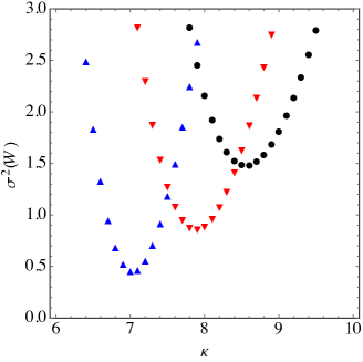
Figure 6: Mean square deviations defined in Eq.(27) as functions of $\varkappa$. Black circles correspond to $W=7$ TeV, red down-triangles to 2.76 TeV and blue up-tangles to 0.9 TeV.

Given the fact that the saturation momentum scales as a power of energy $\overline{Q}_{\mathrm{s}}(W)=(W/Q_{0})^{\lambda_{\mathrm{eff}}}$ we have tried to fit energy dependence of parameters $\kappa_{W}$, $n_{W}$ and $B_{W}$ with generic form $a_{0}(W/Q_{0})^{\alpha}$ with the following result:

$$\kappa_{W} =7.097\;(W/Q_{0})^{0.1000},$$

$$n_{W} =8.199\;(W/Q_{0})^{-0.1005},$$

$$B_{W} =29.76\;(W/Q_{0})^{0.2013}.$$ (28)

This result is surprisingly in line with the effective exponent of the saturation scale which for $\lambda=0.24$ reads $\lambda_{\mathrm{eff}}=0.1071$. Note also that $B\sim\kappa^{2}$ (see definition of $B$ below Eq. (25)), and this dependence is reproduced by the fits of Eqs. (28). Although this energy dependence follows only from the fit to data, and we do not have any model to explain their values, it is a reasonable assumption to take:

$$\kappa_{W} =\kappa_{0}\;\frac{\overline{Q}_{\mathrm{s}}(W)}{Q_{0}},$$

$$n_{W} =n_{0}\;\frac{Q_{0}}{\overline{Q}_{\mathrm{s}}(W)},$$

$$B_{W} =B_{0}\;\frac{\overline{Q}_{\mathrm{s}}^{2}(W)}{Q_{0}^{2}}$$ (29)

where the coefficients $\kappa_{0}$, $n_{0}$ and $B_{0}$ can be read off from Eq. (28). In what follows we shall drop $Q_{0}=1$ GeV/$c$ which was included in (29). Therefore we have:

$$\left.\frac{d^{2}N_{\rm ch}}{dyd^{2}p_{\rm{T}}}\right|_{W} =B_{0}\,\overline{Q}_{\mathrm{s}}^{2}(W)\,\frac{(n_{0}-\overline{Q}_{\mathrm{s}}(W))(n_{0}-2\overline{Q}_{\mathrm{s}}(W))}{n_{0}^{2}}$$

$$\times\left[1+\frac{\varkappa_{0}}{n_{0}}\overline{Q}_{\rm{s}}^{2}(W)\tau^{1/(2+\lambda)}\right]^{-n_{0}/\overline{Q}_{\mathrm{s}}(W)}.$$ (30)

For geometrical scaling to be present we need this function to be inedependent of $W$, i.e. independent of $\overline{Q}_{\mathrm{s}}(W).$ For the energies in question (from a few hundreds GeV up to a few TeV) $\overline{Q}_{\mathrm{s}}(W)$ changes from 0.9 to 1.5. Therefore the factor involving $n_{0}$ is in fact close to 1 and the main energy dependence comes from $\overline{Q}_{\mathrm{s}}^{2}(W)$ in front and from the factor in a square bracket in Eq. (30).

In order to see how GS is reached by Eq. (30) we plot in Fig. 7 ratio $N(\sqrt{\tau},7)/N(\sqrt{\tau},W)$ as a function of $\sqrt{\tau}$ for $W=0.9$, 2.76 and 14 TeV (left panel). Horizontal dashed lines at $1\pm 0.15$ show 15% band around unity which roughly corresponds to the size of the experimental errors $\Delta_{R}$ (10 %) and the accuracy of the fit (5 %) – see Fig. 2. GS is present if theoretical solid curves fall within this interval. We can conclude from Fig. 7 that with this accuracy GS should be seen in the data up to $\sqrt{\tau}\sim 4$ for the whole LHC energy range up to 14 TeV. Should Tsallis parametrization (30) hold for higher energies we might expect shrinking of the maximal $\sqrt{\tau}$ where GS is still present with increasing energy. Given the fact that for fixed $\tau$ transverse momentum $p_{\rm T}$ is an increasing function of energy (see Eq. (11)), this may not immediately mean that the $p_{\rm T}$ window for GS would be shrinking as well.

The same conclusion can be reached by looking at Eq. (30) where $N(\sqrt{\tau},W)/N(\sqrt{\tau},7)$ is plotted as a function of energy for fixed $\tau$. In the right panel of Fig. 7 we plot $N(\sqrt{\tau},W)/N(\sqrt{\tau},7)$ as a function of $W$ for different values of $\sqrt{\tau}=0.2$, 0.5, 1, 2, 3, 4 and 5 shown next to the horizontal axis.

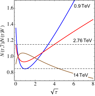
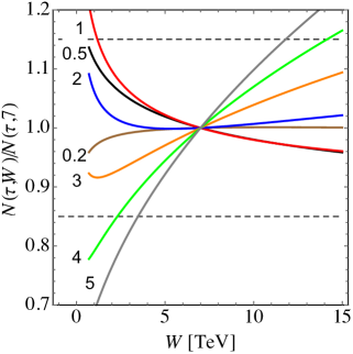
Figure 7: Left panel: Ratios (16) in terms of parametrization of Eq. (30) for $W^{\prime}=0.9$ (blue), 2.76 (red) and 14 TeV (brown). Right panel: multiplicities $N(\sqrt{\tau_{i}},W)$ normalized to $N$ at 7 TeV plotted as functions of $W$ in TeV for fixed values of $\sqrt{\tau_{i}}$ displayed next to the vertical axis.

VI Conclusions

In this paper we have addressed three questions concerning saturation in high energy pp scattering. To this end we have used recent ALICE data on inelastic scattering at the LHC Abelev:2013ala .

The first question concerned the very existence of geometrical scaling in multiplicity distributions. By applying a model-independent method of ratios we have established that GS is indeed present in multiplicity spectra over a limited transverse momentum range up to $\sim 3$ GeV$/c$ with characteristic exponent $\lambda\sim 0.22-0.24$. This exponent is significantly different than in DIS, where $\lambda=0.32$, and also lower than the one extracted from the CMS non-single diffractive data: $\lambda=0.27$. We have proposed the solution to this discrepancy by looking at GS for the inelastic cross-section rather than for the multiplicity distribution. Motivation for this comes from the $k_{\rm T}$ factorized form of the gluon production in pp collisions (4) that leads straightforwardly to Eq. (7) and from the fact that the proportionality factor between the multiplicity and the cross-section (9) is not energy-independent. We have found that the inelastic cross-section scales better than multiplicity up to he maximal transverse momentum that is larger than 4 GeV$/c$ and with the characteristic exponent $\lambda\sim 0.31-0.33$. We have also looked at the UA1 data for $\bar{\rm p}$p scattering and obtained similar value of $\lambda$. We believe that this observation provides a solution to the discrepancy between scaling properties in DIS and in hadronic collisions.

The second question concerned the universal shape of GS and its connection to the Tsallis distribution. We have confirmed that the natural answer to this question is provided by a parametrization where the Tsallis ”temperature” $T$ is proportional to the average saturation scale $\overline{Q}_{\rm s}$ (12) and the remaining Tsallis parameter $n$ should be an energy independent constant. In practice $n$ does depend on energy and this leads to the violation of GS for this particular parametrization.

Finally the third question was whether such a simple solution is admitted by the experimental data. We have found that recent ALICE data on inelastic charged particle multiplicity does not admit the above solution, in agreement with the original claim of Ref. Abelev:2013ala . We have found another parametrization where Tsallis parameter $n$ is inversely proportional to $\overline{Q}_{\rm s}$. This parametrization indeed exhibits GS in the limited energy range, however GS is not obviously extended to higher energies. We have concluded at this point that the solution we found was rather accidental. It will be therefore interesting to see whether this solution will be still present at higher energies of the LHC run II.

References

- (1) A. H. Mueller, arXiv:hep-ph/0111244.
- (2) L. McLerran, Acta Phys. Pol. B 41 (2010) 2799 [arXiv:1011.3203 [hep-ph]].
-
(3)
I. Balitsky,
Nucl. Phys. B 463 (1996) 99;
Y. V. Kovchegov, Phys. Rev. D 60 (1999) 034008 and Phys. Rev. D 61 (2000) 074018. -
(4)
J. Jalilian-Marian, A. Kovner, A. Leonidov, and H. Weigert,
Nucl. Phys. B 504 (1997) 415 and Phys. Rev. D 59
(1998) 014014;
E. Iancu, A. Leonidov, and L. D. McLerran, Nucl. Phys. A 692, (2001) 583 ;
E. Ferreiro, E. Iancu, A. Leonidov, and L. D. McLerran, Nucl. Phys. A 703 (2002) 489. - (5) S. Munier, and R. B. Peschanski, Phys. Rev. Lett. 91 (2003) 232001 [hep-ph/0309177] and Phys. Rev. D 69 (2004) 034008 [hep-ph/0310357].
- (6) A. M. Stasto, K. J. Golec-Biernat and J. Kwiecinski, Phys. Rev. Lett. 86 (2001) 596 [hep-ph/0007192].
- (7) L. D. McLerran, and R. Venugopalan, Phys. Rev. D 49 (1994) 2233 , Phys. Rev. D 49 (1994) 3352 and Phys. Rev. D 50 (1994) 2225 .
- (8) Throughout this paper we shall generically denote by an energy independent function of scaling variable , although in some cases some constant factors are included in without changing notation.
- (9) L. McLerran and M. Praszalowicz, Acta Phys. Polon. B 41 (2010) 1917 [arXiv:1006.4293 [hep-ph]] and Acta Phys. Polon. B 42 (2011) 99 [arXiv:1011.3403 [hep-ph]].
- (10) M. Praszalowicz and T. Stebel, JHEP 1303 (2013) 090 [arXiv:1211.5305 [hep-ph]] and JHEP 1304 (2013) 169 [arXiv:1302.4227 [hep-ph]].
- (11) M. Praszalowicz, Phys. Rev. D 87 (2013) 071502 [arXiv:1301.4647 [hep-ph]].
- (12) B. B. Abelev et al. [ALICE Collaboration], Eur. Phys. J. C 73 (2013) 12, 2662 [arXiv:1307.1093 [nucl-ex]].
-
(13)
C. Tsallis, J. Stat. Phys. 52 (1988) 479 and Eur. Phys. J. A 40 (2009) 257;
T. S. Biró, G. Purcsel, and K. Ürmössy, Eur. Phys. J. bfA 40, 325 (2009). - (14) C. Y. Wong and G. Wilk, Acta Phys. Polon. B 43 (2012) 2047 [arXiv:1210.3661 [hep-ph]] and Phys. Rev. D 87 (2013) 11, 114007 [arXiv:1305.2627 [hep-ph]] and arXiv:1309.7330 [hep-ph].
-
(15)
L. J. L. Cirto, C. Tsallis, C. Y. Wong and G. Wilk,
arXiv:1409.3278 [hep-ph];
C. Y. Wong, G. Wilk, L. J. L. Cirto and C. Tsallis, EPJ Web Conf. 90 (2015) 04002 [arXiv:1412.0474 [hep-ph]]. -
(16)
J. Cleymans, G. I. Lykasov, A. S. Parvan, A. S. Sorin, O. V. Teryaev and D. Worku,
Phys. Lett. B 723 (2013) 351
[arXiv:1302.1970 [hep-ph]];
M. D. Azmi and J. Cleymans, J. Phys. G 41 (2014) 065001 [arXiv:1401.4835 [hep-ph]];
L. Marques, J. Cleymans and A. Deppman, Phys. Rev. D 91 (2015) 054025 [arXiv:1501.00953 [hep-ph]]. - (17) L. V. Gribov, E. M. Levin and M. G. Ryskin, Phys. Lett. B 100 (1981) 173.
- (18) A. Szczurek, Acta Phys. Polon. B 35 (2004) 161 [hep-ph/0311175].
- (19) K.J. Golec-Biernat and M. Wüsthoff, Phys. Rev. D bf59 (1998) 014017 [hep-ph/9807513] and Phys. Rev. D bf60 (1999) 114023 [hep-ph/9903358].
- (20) D. Kharzeev, E. Levin and M. Nardi, Nucl. Phys. A 730 (2004) 448 [Nucl. Phys. A 743 (2004) 329] [hep-ph/0212316] and Nucl. Phys. A 747 (2005) 609 [hep-ph/0408050].
- (21) H. Kowalski and D. Teaney, Phys. Rev. D 68 (2003) 114005 [hep-ph/0304189].
- (22) P. Tribedy and R. Venugopalan, Nucl. Phys. A 850 (2011) 136 [Nucl. Phys. A 859 (2011) 185] [arXiv:1011.1895 [hep-ph]].
- (23) E. Levin and A. H. Rezaeian, Phys. Rev. D 83 (2011) 114001 [arXiv:1102.2385 [hep-ph]].
-
(24)
Ya.I. Azimov, Yu.L. Dokshitzer, V.A. Khoze and S.I. Troian, Z. Phys. C 27 (1985) 65;
Yu. L. Dokshitzer, V. A. Khoze and S. I. Troyan, J. Phys. G 17 (1991) 1585;
V.A. Khoze and W. Ochs, Int. J. Mod. Phys. A 12 (1997) 2949;
S. Lupia and W. Ochs, Phys. Lett. B 418 (1998) 214. -
(25)
L. McLerran and M. Praszalowicz,
Phys. Lett. B 741 (2015) 246
[arXiv:1407.6687 [hep-ph]];
M. Praszalowicz, AIP Conf. Proc. 1654 (2015) 080001 [arXiv:1410.5220 [hep-ph]]. - (26) C. Albajar et al. [UA1 Collaboration], Nucl. Phys. B 335 (1990) 261.
- (27) R. Hagedorn, Nuovo Cim. Suppl. 3 (1965) 147.
- (28) S. Chatrchyan itet al. [CMS Collaboration], Eur. Phys. J. C 72, 2164 (2012) [arXiv:1207.4724 [hep-ex]].
- (29) M. Praszalowicz, Phys. Lett. B 727 (2013) 461 [arXiv:1308.5911 [hep-ph]].