Grand Unification in the Spectral Pati–Salam Model

Abstract

We analyze the running at one-loop of the gauge couplings in the spectral Pati–Salam model that was derived in the framework of noncommutative geometry. There are a few different scenario’s for the scalar particle content which are determined by the precise form of the Dirac operator for the finite noncommutative space. We consider these different scenarios and establish for all of them unification of the Pati–Salam gauge couplings. The boundary conditions are set by the usual RG flow for the Standard Model couplings at an intermediate mass scale at which the Pati–Salam symmetry is broken.

I Introduction

This paper builds on two recent discoveries in the noncommutative geometry approach to particle physics: we showed in CCS13b how to obtain inner fluctuations of the metric without having to assume the order one condition on the Dirac operator. Moreover the original argument by classification CC07b of finite geometries $F$ that can provide the fine structure of Euclidean space-time as a product $M\times F$ (where $M$ is a usual $4$-dimensional Riemannian space) has now been replaced by a much stronger uniqueness statement CCM14 ; CCM15 . This new result shows that the algebra

$$M_{2}(\mathbb{H})\oplus M_{4}(\mathbb{C}),$$ (1)

where $\mathbb{H}$ are the quaternions, appears uniquely when writing the higher analogue of the Heisenberg commutation relations. This analogue is written in terms of the basic ingredients of noncommutative geometry where one takes a spectral point of view, encoding geometry in terms of operators on a Hilbert space $\mathcal{H}$. In this way, the inverse line element is an unbounded self-adjoint operator $D$. The operator $D$ is the tensor sum of the usual Dirac operator on $M$ and a ‘finite Dirac operator’ on $F$, which is simply a hermitian matrix $D_{F}$. The usual Dirac operator involves $\gamma$ matrices which allow one to combine the momenta into a single operator. The higher analogue of the Heisenberg relations puts the spatial variables on similar footing by combining them into a single operator $Y$ using another set of $\gamma$ matrices and it is in this process that the algebra (1) appears canonically and uniquely in dimension $4$. We refer to CCM14 ; CCM15 for a detailed account. What matters for the present paper is that the above process leads without arbitrariness to the Pati–Salam PS74 gauge group $SU(2)_{R}\times SU(2)_{L}\times SU(4)$, together with the corresponding gauge fields and a scalar sector, all derived as inner perturbations of $D$ CCS13b . Note that the scalar sector can not be chosen freely, in contrast to the early work on Pati–Salam unification Eli76 ; Eli77 ; Bar82 ; CMP84 . In fact, there are only a few possibilities for the precise scalar content, depending on the assumptions made on the finite Dirac operator.

From the spectral action principle, the dynamics and interactions are described by the spectral action CC96 ; CC97 ,

$$\mathrm{tr}(f(D_{A}/\Lambda))$$ (2)

where $\Lambda$ is a cutoff scale and $f$ an even and positive function. In the present case, it can be expanded using heat kernel methods,

$$\mathrm{tr}(f(D_{A}/\Lambda))\sim F_{4}\Lambda^{4}a_{0}+F_{2}\Lambda^{2}a_{2}+F_{0}a_{4}+\cdots$$ (3)

where $F_{4},F_{2},F_{0}$ are coefficients related to the function $f$ and $a_{k}$ are Seeley deWitt coefficients, expressed in terms of the curvature of $M$ and (derivatives of) the gauge and scalar fields. This action is interpreted as an effective field theory for energies lower than $\Lambda$.

One important feature of the spectral action is that it gives the usual Pati–Salam action with unification of the gauge couplings CCS13b (cf. Eq. (43) below). This is very similar to the case of the spectral Standard Model CCM07 where there is unification of gauge couplings. Since it is well known that the SM gauge couplings do not meet exactly, it is crucial to investigate the running of the Pati–Salam gauge couplings beyond the Standard Model and to find a scale $\Lambda$ where there is grand unification:

$$g_{R}(\Lambda)=g_{L}(\Lambda)=g(\Lambda).$$ (4)

This would then be the scale at which the spectral action (3) is valid as an effective theory. There is a hierarchy of three energy scales: SM, an intermediate mass scale $m_{R}$ where symmetry breaking occurs and which is related to the neutrino Majorana masses ($10^{11}-10^{13}$Gev), and the GUT scale $\Lambda$.

For simplicity, we restrict our analysis to the running of the gauge couplings at one-loop. Indeed, at two loops, the gauge and scalar couplings are mixed and influence each other. Moreover, the running of the scalar mass terms can not be trusted at all because of quadratic divergences.

Thus, we analyze the running of the gauge couplings according to the usual (one-loop) RG equation where each takes the form

$$16\pi^{2}\frac{dg}{dt}=-bg^{3}.$$ (5)

The coefficient $b$ is determined by the particle content and their representation theory CEL74 ; MV83 ; MV84 ; MV85 for which we use KP81 as well as the program PyR@TE. As mentioned before, depending on the assumptions on $D_{F}$, one may vary to a limited extent the scalar particle content, consisting of either composite or fundamental scalar fields. We will not limit ourselves to a specific model but consider all cases separately. In fact, we establish grand unification for all of them, thus confirming validity of the spectral action at the corresponding scale, independent of the specific form of $D_{F}$.

II Spectral Pati–Salam and grand unification

One of the pressing questions at present is whether there is new physics beyond the Standard Model. The success of the spectral construction of the Standard Model, predicting its particle content, including gauge fields, Higgs fields as well as a singlet whose vev gives Majorana mass to the right handed neutrino, is a strong signal that we are on the right track. The route that led to this conclusion starts with classifying the algebras of the finite space. The results show that the only algebras which solve the fermion doubling problem are of the form $M_{2a}(\mathbb{C})\oplus M_{2a}(\mathbb{C})$ where $a$ is an even integer. An arbitrary symplectic constraint is imposed on the first algebra restricting it from $M_{2a}(\mathbb{C})$ to $M_{a}(\mathbb{H}).$ The first non-trivial algebra one can consider is for $a=2$ with the algebra CC07b

$$M_{2}(\mathbb{H})\oplus M_{4}(\mathbb{C}).$$ (6)

Coincidentally, and as explained in the introduction, the above algebra comes out as a solution of the two-sided Heisenberg quantization relation between the Dirac operator $D$ and the two maps from the four spin-manifold and the two four spheres $S^{4}\times S^{4}$ CCM14 ; CCM15 . This removes the arbitrary symplectic constraint and replaces it with a relation that quantize the four-volume in terms of two quanta of geometry and have far reaching consequences on the structure of space-time.

The existence of the chirality operator $\gamma$ that commutes with the algebra breaks the quaternionic matrices $M_{2}(\mathbb{H})$ to the diagonal subalgebra and leads us to consider the finite algebra

$$\mathcal{A}_{F}=\mathbb{H}_{R}\oplus\mathbb{H}_{L}\oplus M_{4}(\mathbb{C}).$$ (7)

The Pati–Salam gauge group $SU(2)_{R}\times SU(2)_{L}\times SU(4)$ is obtained as the inner automorphism group of $\mathcal{A=C}^{\infty}\left(M\right)\otimes\mathcal{A}_{F}$, and the corresponding gauge bosons appear as inner perturbations of the (spacetime) Dirac operator CCS13b .

Next, an element of the Hilbert space $\Psi\in\mathcal{H}$ is represented by

$$\Psi_{M}=\left(\begin{array}[c]{c}\psi_{A}\\ \psi_{A^{{}^{\prime}}}\end{array}\right),\quad\psi_{A^{\prime}}=\psi_{A}^{c}$$ (8)

where $\psi_{A}^{c}$ is the conjugate spinor to $\psi_{A}.$ Thus all primed indices $A^{\prime}$ correspond to the Hilbert space of conjugate spinors. It is acted on by both the left algebra $M_{2}\left(\mathbb{H}\right)$ and the right algebra $M_{4}\left(\mathbb{C}\right)$. Therefore the index $A$ can take $16$ values and is represented by

$$A=\alpha I$$ (9)

where the index $\alpha$ is acted on by quaternionic matrices and the index $I$  by $M_{4}\left(\mathbb{C}\right)$ matrices. Moreover, when the grading breaks $M_{2}\left(\mathbb{H}\right)$ into $\mathbb{H}_{R}\oplus\mathbb{H}_{L}$ the index $\alpha$ is decomposed to $\alpha=\overset{.}{a},a$ where $\overset{.}{a}=\overset{.}{1},\overset{.}{2}$ (dotted index) is acted on by the first quaternionic algebra $\ \mathbb{H}_{R}$ and $a=1,2$ is acted on by the second quaternionic algebra $\ \mathbb{H}_{L}$. When $M_{4}\left(\mathbb{C}\right)$ breaks into $\mathbb{C}\oplus M_{3}\left(\mathbb{C}\right)$ (due to symmetry breaking or through the use of the order one condition as in CC07b ) the index $I$ is decomposed into $I=1,i$ and thus distinguishing leptons and quarks, where the $1$ is acted on by the $\mathbb{C}$ and the $i$ by $M_{3}\left(\mathbb{C}\right).$ Therefore the various components of the spinor $\psi_{A}$ are

$$\psi_{\alpha I} =\left(\begin{array}[c]{cccc}\nu_{R}&u_{iR}&\nu_{L}&u_{iL}\\ e_{R}&d_{iR}&e_{L}&d_{iL}\end{array}\right),\qquad i=1,2,3$$ (12)

$$=\left(\psi_{\overset{.}{a}1},\psi_{\overset{.}{a}i},\psi_{a1},\psi_{ai}\right),\qquad a=1,2,\quad\overset{.}{a}=\overset{.}{1},\overset{.}{2}$$

This is a general prediction of the spectral construction that there is $16$ fundamental Weyl fermions per family, $4$ leptons and $12$ quarks.

The (finite) Dirac operator can be written in matrix form

$$D_{F}=\left(\begin{array}[c]{cc}D_{A}^{B}&D_{A}^{B^{{}^{\prime}}}\\ D_{A^{{}^{\prime}}}^{B}&D_{A^{{}^{\prime}}}^{B^{{}^{\prime}}}\end{array}\right),$$ (13)

and must satisfy the properties

$$\gamma_{F}D_{F}=-D_{F}\gamma_{F}\qquad J_{F}D_{F}=D_{F}J_{F}$$ (14)

where $J_{F}^{2}=1.$ A matrix realization of $\gamma_{F}$ and $J_{F}$ are given by

$$\gamma_{F}=\left(\begin{array}[c]{cc}G_{F}&0\\ 0&-\overline{G}_{F}\end{array}\right),\qquad G_{F}=\left(\begin{array}[c]{cc}1_{2}&0\\ 0&-1_{2}\end{array}\right),\qquad J_{F}=\left(\begin{array}[c]{cc}0_{4}&1_{4}\\ 1_{4}&0_{4}\end{array}\right)\circ\mathrm{cc}$$ (15)

where $\mathrm{cc}$ stands for complex conjugation. These relations, together with the hermiticity of $D$ imply the relations

$$\left(D_{F}\right)_{A^{{}^{\prime}}}^{B^{{}^{\prime}}}=\left(\overline{D}_{F}\right)_{A}^{B}\,\qquad\left(D_{F}\right)_{A^{{}^{\prime}}}^{B}=\left(\overline{D}_{F}\right)_{B}^{A^{\prime}}$$ (16)

and have the following zero components CC10

$$\left(D_{F}\right)_{aI}^{bJ} =0=\left(D_{F}\right)_{\overset{.}{a}I}^{\overset{.}{b}J}$$ (17)

$$\left(D_{F}\right)_{aI}^{\overset{.}{b}^{\prime}J^{\prime}} =0=\left(D_{F}\right)_{\overset{.}{a}I}^{b^{\prime}J\prime}$$ (18)

leaving the components $\left(D_{F}\right)_{aI}^{\overset{.}{b}J}$, $\left(D_{F}\right)_{aI}^{b^{\prime}J^{\prime}}$ and $\left(D_{F}\right)_{\overset{.}{a}I}^{\overset{.}{b}^{\prime}J^{\prime}}$ arbitrary. These restrictions lead to important constraints on the structure of the connection that appears in the inner fluctuations of the Dirac operator. In particular the operator $D$ of the full noncommutative space given by

$$D=D_{M}\otimes 1+\gamma_{5}\otimes D_{F}$$ (19)

gets modified to

$$D_{A}=D+A_{\left(1\right)}+JA_{\left(1\right)}J^{-1}+A_{\left(2\right)}$$ (20)

where

$$A_{\left(1\right)}={\displaystyle\sum}a\left[D,b\right],\,\qquad A_{2}={\displaystyle\sum}\widehat{a}\left[A_{\left(1\right)},\widehat{b}\right],\qquad\widehat{a}=JaJ^{-1}$$ (21)

We have shown in CCS13b that components of the connection $A$ which are tensored with the Clifford gamma matrices $\gamma^{\mu}$ are the gauge fields of the Pati–Salam model with the symmetry of $SU\left(2\right)_{R}\times SU\left(2\right)_{L}\times SU\left(4\right).$ On the other hand, the non-vanishing components of the connection which are tensored with the gamma matrix $\gamma_{5}$ are given by

$$\left(A\right)_{aI}^{\overset{.}{b}J}\equiv\gamma_{5}\Sigma_{aI}^{\overset{.}{b}J},\qquad\left(A\right)_{aI}^{b^{\prime}J^{\prime}}=\gamma_{5}H_{aIbJ},\qquad\left(A\right)_{\overset{.}{a}I}^{\overset{.}{b}^{\prime}J^{\prime}}\equiv\gamma_{5}H_{\overset{.}{a}I\overset{.}{b}J}$$ (22)

where $H_{aIbJ}=H_{bJaI}$ and $H_{\overset{.}{a}I\overset{.}{b}J}=H_{\overset{.}{b}J\overset{.}{a}I}$, which is the most general Higgs structure possible. These correspond to the representations with respect to $SU\left(2\right)_{R}\times SU\left(2\right)_{L}\times SU\left(4\right):$

$$\Sigma_{aI}^{\overset{.}{b}J} =\left(2_{R},2_{L},1\right)+\left(2_{R},2_{L},15\right)$$ (23)

$$H_{aIbJ} =\left(1_{R},1_{L},6\right)+\left(1_{R},3_{L},10\right)$$ (24)

$$H_{\overset{.}{a}I\overset{.}{b}J} =\left(1_{R},1_{L},6\right)+\left(3_{R},1_{L},10\right)$$ (25)

We note, however, that the inner fluctuations form a semi-group and if a component $\left(D_{F}\right)_{aI}^{\overset{.}{b}J}$ or $\left(D_{F}\right)_{aI}^{b^{\prime}J^{\prime}}$ or $\left(D_{F}\right)_{\overset{.}{a}I}^{\overset{.}{b}^{\prime}J^{\prime}}$ vanish, then the corresponding $A$ field will also vanish. We distinguish three cases: 1) Left-right symmetric Pati–Salam model with fundamental Higgs fields $\Sigma_{aI}^{\overset{.}{b}J},$ $H_{aIbJ}$ and $H_{\overset{.}{a}I\overset{.}{b}J}.$ In this model the field $H_{aIbJ}$ should have a zero vev. 2) A Pati–Salam model where the Higgs field $H_{aIbJ}$ that couples to the left sector is set to zero which is desirable because there is no symmetry between the left and right sectors at low energies. 3) If one starts with $\left(D_{F}\right)_{aI}^{\overset{.}{b}J}$ or $\left(D_{F}\right)_{aI}^{b^{\prime}J^{\prime}}$ or $\left(D_{F}\right)_{\overset{.}{a}I}^{\overset{.}{b}^{\prime}J^{\prime}}$ whose values are given by those that were derived for the Standard Model, then the Higgs fields $\Sigma_{aI}^{\overset{.}{b}J},$ $H_{aIbJ}$ and $H_{\overset{.}{a}I\overset{.}{b}J}$ will become composite and expressible in terms of more fundamental fields $\Sigma_{I}^{J},$ $\Delta_{\overset{.}{a}J}$ and $\phi_{\overset{.}{a}}^{b}$ . We refer to this as the composite model.

Depending on the precise particle content we determine the coefficients $b_{R},b_{L},b$ in (5) that control the RG flow of the Pati–Salam gauge couplings $g_{R},g_{L},g$. We run them to look for unification of the coupling $g_{R}=g_{L}=g$. The boundary conditions are taken at the intermediate mass scale $\mu=m_{R}$ to be the usual (e.g. (Moh86, , Eq. (5.8.3)))

$$\frac{1}{g_{1}^{2}}=\frac{2}{3}\frac{1}{g^{2}}+\frac{1}{g_{R}^{2}},\qquad\frac{1}{g_{2}^{2}}=\frac{1}{g_{L}^{2}},\qquad\frac{1}{g_{3}^{2}}=\frac{1}{g^{2}},$$ (26)

in terms of the Standard Model gauge couplings $g_{1},g_{2},g_{3}$. At the mass scale $m_{R}$ the Pati–Salam symmetry is broken to that of the Standard Model, and we take it to be the same scale that is present in the see-saw mechanism. It should thus be of the order $10^{11}-10^{13}$Gev. We now discuss the three models, in order of complexity.

II.1 Pati–Salam with composite Higgs fields

$$\begin{array}[c]{c|ccc}\text{particle}&SU(2)_{R}&SU(2)_{L}&SU(4)\\ \hline\cr\phi_{\dot{a}}^{b}&2&2&1\\ \Delta_{\dot{a}I}&2&1&4\\ \hline\cr\Sigma_{J}^{I}&1&1&15\end{array}$$

Table 1: Pati–Salam scalar particle content and their representations for a first-order Dirac operator. The field $\Sigma_{J}^{I}$ in the last row is decoupled if there is quark-lepton coupling unification.

We first consider the case of a finite Dirac operator for which the Standard Model subalgebra $\mathbb{C}\oplus\mathbb{H}_{L}\oplus M_{3}(\mathbb{C})\subset\mathcal{A}_{F}$ satisfies the first-order condition CC07b . This condition is extremely constraining and forces the couplings of the right-handed neutrino to be with a singlet. In this case, the off-diagonal term in (13) becomes

$$D_{\alpha I}^{\beta^{\prime}K^{\prime}}=\delta_{\alpha}^{\overset{.}{1}}\delta_{\overset{.}{1^{\prime}}}^{\beta^{\prime}}\delta_{I}^{1}\delta_{1^{\prime}}^{K^{\prime}}k^{\ast\nu_{R}},$$ (27)

and the diagonal structure of $D_{F}$ is determined by the following sub-matrices CC10

$$D_{\alpha 1}^{\quad\beta 1} =\left(\begin{array}[c]{cc}0&D_{a1}^{\overset{.}{b}1}\\ D_{\overset{.}{a}1}^{b1}&0\end{array}\right),\quad D_{a1}^{\overset{.}{b}1}=\left(D_{\overset{.}{a}1}^{b1}\right)^{\ast}\equiv D_{a\left(l\right)}^{\overset{.}{b}}$$ (30)

$$D_{\alpha i}^{\quad\beta j} =\left(\begin{array}[c]{cc}0&D_{a\left(q\right)}^{\overset{.}{b}}\delta_{i}^{j}\\ D_{\overset{.}{a}\left(q\right)}^{b}\delta_{i}^{j}&0\end{array}\right),\quad D_{\overset{.}{a}\left(q\right)}^{b}=\left(D_{a\left(q\right)}^{\overset{.}{b}}\right)^{\ast}$$ (33)

where

$$D_{a\left(q\right)}^{\overset{.}{b}}=\left(\begin{array}[c]{cc}k^{\ast u}&0\\ 0&k^{\ast d}\end{array}\right).$$

The Yukawa couplings $k^{\nu},$ $k^{e},$ $k^{u},$ $k^{d}$ are $3\times 3$ matrices in generation space. Notice that this structure gives Dirac masses to all the fermions, but Majorana masses only for the right-handed neutrinos. One can also consider the special case of lepton and quark unification by equating $k^{\nu}=k^{u},k^{e}=k^{d}$ which imply some simplifications.

The inner perturbations of the finite Dirac operator of the above type were determined in CCS13b to be composite fields $\Sigma_{\overset{.}{a}I}^{bJ}$ and $H_{\overset{.}{a}I\overset{.}{b}J}$, depending on fundamental Higgs fields $\phi_{\overset{.}{a}}^{b}$, $\Sigma_{I}^{J}$ and $\Delta_{\overset{.}{a}J}$ in the following way:

$$\Sigma_{\overset{.}{a}I}^{bJ} =\left(k^{\nu}\phi_{\overset{.}{a}}^{b}+k^{e}\widetilde{\phi}_{\overset{.}{a}}^{b}\right)\Sigma_{I}^{J}+\left(k^{u}\phi_{\overset{.}{a}}^{b}+k^{d}\widetilde{\phi}_{\overset{.}{a}}^{b}\right)\left(\delta_{I}^{J}-\Sigma_{I}^{J}\right),$$

$$H_{\overset{.}{a}I\overset{.}{b}J} =k^{\ast\nu_{R}}\Delta_{\overset{.}{a}J}\Delta_{\overset{.}{b}I}.$$ (34)

The field $\widetilde{\phi}_{\overset{.}{a}}^{b}$ is not an independent field and is given by

$$\widetilde{\phi}_{\overset{.}{a}}^{b}=\sigma_{2}\overline{\phi}_{\overset{.}{a}}^{b}\sigma_{2}.$$ (35)

We have listed the fundamental Higgs fields and their representations in Table 1. We first assume that there is lepton quark unification, so that the $\Sigma_{I}^{J}$ is decoupled.

The $\beta$-functions for the Pati–Salam couplings $g_{R},g_{L},g$ with the above particle content are found to be

$$(b_{R},b_{L},b)=\left(\frac{7}{3},3,\frac{31}{3}\right).$$ (36)

The solutions of the RG-equations are easily found to be

$$g_{R}(\mu)^{-2} =g_{R}(m_{R})^{-2}+\frac{1}{8\pi^{2}}\frac{7}{3}\log\frac{\mu}{m_{R}},$$ (37)

$$g_{L}(\mu)^{-2} =g_{L}(m_{R})^{-2}+\frac{1}{8\pi^{2}}3\log\frac{\mu}{m_{R}},$$ (38)

$$g(\mu)^{-2} =g(m_{R})^{-2}+\frac{1}{8\pi^{2}}\frac{31}{3}\log\frac{\mu}{m_{R}},$$ (39)

We impose the boundary conditions (26) at the mass scale $\mu=m_{R}$.

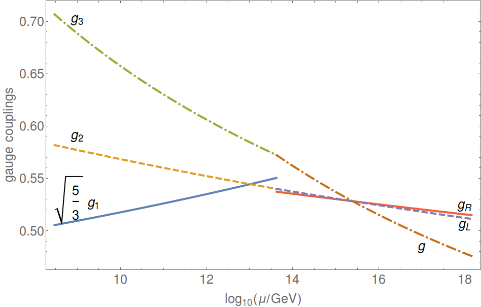
Figure 1: Running of coupling constants for the spectral Pati–Salam model with composite Higgs fields: $g_{1},g_{2},g_{3}$ for $\mu<m_{R}$ and $g_{R},g_{L},g$ for $\mu>m_{R}$ with unification scale $\Lambda\approx 2.5\times 10^{15}\operatorname{GeV}$ for $m_{R}=4.25\times 10^{13}\operatorname{GeV}$.

As a first approximation, we adopt the usual running of the SM gauge couplings, leaving a full analysis of the effect of the scalar fields after Pati–Salam symmetry breaking to future work. Also, we ignore the presence of non-renormalizable terms in the spectral action for the composite model. Then, after experimenting with different values of $m_{R}$, we find a unification scale $\Lambda\approx 2.5\times 10^{15}$Gev if we set $m_{R}=4.25\times 10^{13}$Gev (Figure 1).

If the scalar field $\Sigma_{I}^{J}$ is not decoupled —in other words, if there is no lepton-quark coupling unification— then there is an additional scalar $(1_{R},1_{L},15)$ irreducible representation contributing to the $\beta$-function, giving a slightly different $(b_{R},b_{L},b)=\left(\frac{7}{3},3,9\right)$. This in turn gives a unification scale $\Lambda\approx 6.3\times 10^{15}$Gev for $m_{R}=4.1\times 10^{13}$Gev.

II.2 Pati–Salam with fundamental Higgs fields

Next, we consider the case of a more general finite Dirac operator, not satisfying the first-order condition with respect to the Standard Model subalgebra. We begin with the special case where

$$\left(D_{F}\right)_{aI}^{b^{\prime}J^{\prime}}=0$$ (40)

which implies that the Higgs field $H_{aIbJ}=0.$ The inner perturbations $\Sigma_{\overset{.}{a}I}^{bJ}$ and $H_{\overset{.}{a}I\overset{.}{b}J}$ are now themselves fundamental Higgs fields (CCS13b, , Sect. 5) and their representations are listed in Table 2. The $\beta$-functions are computed to be

$$(b_{R},b_{L},b)=\left(-\frac{26}{3},-2,2\right)$$ (41)

Note that the $SU(2)_{R}$ and $SU(2)_{L}$-sectors are not asymptotically free, due to the large scalar sector. Nevertheless, we can still run the gauge couplings with the boundary values set by (26). Adopting the same approximation as in the previous section, this results in Figure 2. The unification scale is $\Lambda\approx 6.3\times 10^{16}$Gev if we set $m_{R}=1.5\times 10^{11}$Gev.

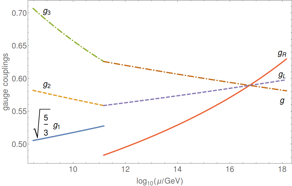
Figure 2: Running of coupling constants for the spectral Pati–Salam model with fundamental Higgs fields: $g_{1},g_{2},g_{3}$ for $\mu<m_{R}$ and $g_{R},g_{L},g$ for $\mu>m_{R}$ with unification scale $\Lambda\approx 6.3\times 10^{16}\operatorname{GeV}$ for $m_{R}=1.5\times 10^{11}\operatorname{GeV}$.

$$\begin{array}[c]{c|ccc}\text{particle}&SU(2)_{R}&SU(2)_{L}&SU(4)\\ \hline\cr\Sigma_{\dot{a}J}^{bJ}&2&2&1+15\\ H_{\dot{a}I\dot{b}J}\bigg{\{}&\begin{array}[c]{cc}3&\\ 1&\end{array}&\begin{array}[c]{cc}1&\\ 1&\end{array}&\begin{array}[c]{cc}10&\\ 6&\end{array}\end{array}$$

Table 2: Pati–Salam scalar particle content and their representations for a general finite Dirac operator.

II.3 Left-right symmetric Pati–Salam with fundamental Higgs fields

As a final possibility we consider the most general case for $D_{F}$ which gives in addition to the fundamental Higgs fields in Table 2 the field $H_{aIbJ}$ in the $(1_{R},3_{L},10)+(1_{R},1_{L},6)$ representation. The $\beta$-functions become

$$(b_{R},b_{L},b)=\left(-\frac{26}{3},-\frac{26}{3},-\frac{4}{3}\right)$$ (42)

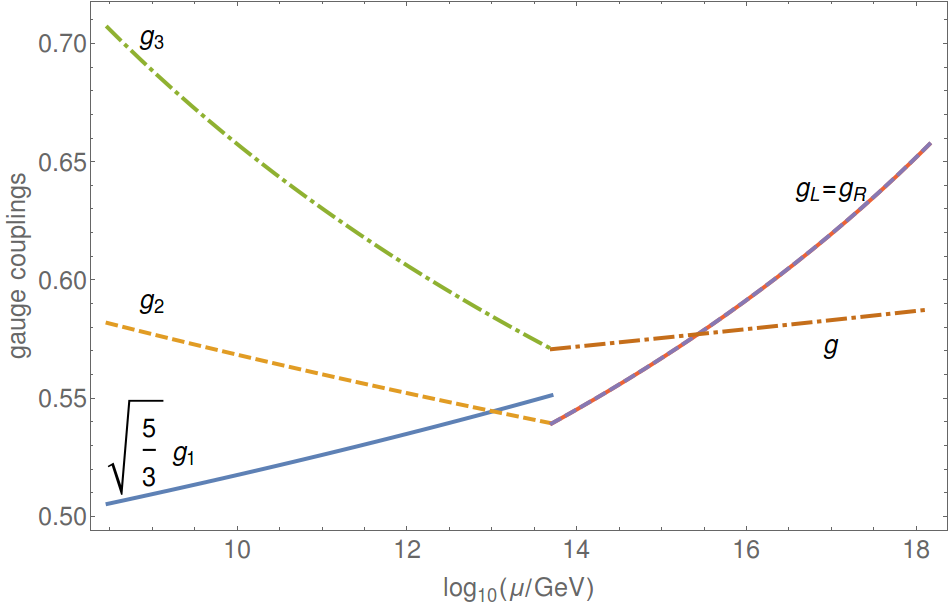
Figure 3: Running of coupling constants for the left-right symmetric spectral Pati–Salam model: $g_{1},g_{2},g_{3}$ for $\mu<m_{R}$ and $g_{R},g_{L},g$ for $\mu>m_{R}$ with unification scale $\Lambda\approx 2.7\times 10^{15}\operatorname{GeV}$ for $m_{R}=5.1\times 10^{13}\operatorname{GeV}$.

Adopting once more the approximation that we made use of in the previous sections, we run the Pati–Salam gauge couplings from $m_{R}$, resulting in Figure 3. We find the unification scale to be $\Lambda\approx 2.7\times 10^{15}$Gev if we set $m_{R}=5.1\times 10^{13}$Gev.

III Conclusions

We have analyzed the running of the Pati–Salam gauge couplings for the spectral model, considering different scalar field contents corresponding to the assumptions made on the finite Dirac operator. We stress that the number of possible models is quite restrictive and that one can not freely choose the particle content. We have identified the three main models, although there exists small variations on them. The different possibilities correspond to restrictions on the geometry of the finite space $F$. In all the models considered here, we establish unification of the gauge couplings, with boundary conditions set by the usual Standard Model gauge couplings at an intermediate mass scale.

Besides the direct physical interest of such grand unification, it also determines the scale at which the asymptotic expansion of Equation (3) is actually valid as an effective theory. In order to see this, note that the scale-invariant term $F_{0}a_{4}$ in (3) for the spectral Pati–Salam model contains the terms CCS13b :

$$\frac{F_{0}}{2\pi^{2}}\int\left(g_{L}^{2}\left(W_{\mu\nu L}^{\alpha}\right)^{2}+g_{R}^{2}\left(W_{\mu\nu R}^{\alpha}\right)^{2}+g^{2}\left(V_{\mu\nu}^{m}\right)^{2}\right).$$ (43)

Normalizing this to give the Yang–Mills Lagrangian demands

$$\frac{F_{0}}{2\pi^{2}}g_{L}^{2}=\frac{F_{0}}{2\pi^{2}}g_{R}^{2}=\frac{F_{0}}{2\pi^{2}}g^{2}=\frac{1}{4},$$ (44)

which requires gauge coupling unification, $g_{R}=g_{L}=g$. Note that the similar result for the Standard Model gauge couplings does not hold (at least at the one-loop level) because the three couplings actually do not meet, even though they are required to be unified in the spectral action CC96 . We consider this to be strong evidence for the spectral Pati–Salam model as a realistic possibility to go beyond the Standard Model.

To summarize, the spectral construction of particle physics models based on a spectral triple with a noncommutative space with metric dimension four and whose finite part has KO dimension $6$ leads directly to a family of Pati–Salam models with gauge symmetry $SU\left(2\right)_{R}\times SU\left(2\right)_{L}\times SU\left(4\right)$ and well defined Higgs structure. Breaking of $SU\left(2\right)_{R}\times SU\left(4\right)$ to $U\left(1\right)\times SU\left(3\right)$ occurs at some scale $m_{R}\sim 10^{11}-10^{13}$ Gev with a unification scale where the three coupling constants meet of the order of $10^{16}$ Gev. All these breakings will have the Standard Model as an effective theory at low energies.

References

• (1) V. D. Barger, E. Ma, and K. Whisnant. General analysis of a possible second weak neutral current in gauge models. Phys. Rev. D26 (1982) 2378.
• (2) A. H. Chamseddine and A. Connes. Universal formula for noncommutative geometry actions: Unifications of gravity and the Standard Model. Phys. Rev. Lett. 77 (1996) 4868–4871.
• (3) A. H. Chamseddine and A. Connes. The spectral action principle. Commun. Math. Phys. 186 (1997) 731–750.
• (4) A. H. Chamseddine and A. Connes. Why the Standard Model. J. Geom. Phys. 58 (2008) 38–47.
• (5) A. H. Chamseddine and A. Connes. Noncommutative geometry as a framework for unification of all fundamental interactions including gravity. Part I. Fortsch. Phys. 58 (2010) 553–600.
• (6) A. H. Chamseddine, A. Connes, and M. Marcolli. Gravity and the Standard Model with neutrino mixing. Adv. Theor. Math. Phys. 11 (2007) 991–1089.
• (7) A. H. Chamseddine, A. Connes, and V. Mukhanov. Geometry and the quantum: Basics. JHEP 1412 (2014) 098.
• (8) A. H. Chamseddine, A. Connes, and V. Mukhanov. Quanta of geometry: Noncommutative aspects. Phys. Rev. Lett. 114 (2015) 091302.
• (9) A. H. Chamseddine, A. Connes, and W. D. van Suijlekom. Beyond the spectral Standard Model: Emergence of Pati-Salam unification. JHEP 1311 (2013) 132.
• (10) D. Chang, R. Mohapatra, and M. Parida. A new approach to left-right symmetry breaking in unified gauge theories. Phys. Rev. D30 (1984) 1052.
• (11) T. Cheng, E. Eichten, and L.-F. Li. Higgs phenomena in asymptotically free gauge theories. Phys. Rev. D9 (1974) 2259.
• (12) V. Elias. Coupling constant renormalization in unified gauge theories containing the Pati-Salam model. Phys. Rev. D14 (1976) 1896.
• (13) V. Elias. Gauge coupling constant magnitudes in the Pati-Salam model. Phys. Rev. D16 (1977) 1586.
• (14) M. Machacek and M. Vaughn. Two-loop renormalization group equations in a general quantum field theory : (i). Wave function renormalization. Nucl. Phys. B 222 (1983) 83 – 103.
• (15) M. Machacek and M. Vaughn. Two-loop renormalization group equations in a general quantum field theory (ii). Yukawa couplings. Nucl. Phys. B 236 (1984) 221 – 232.
• (16) M. Machacek and M. Vaughn. Two-loop renormalization group equations in a general quantum field theory : (iii). Scalar quartic couplings. Nucl. Phys. B 249 (1985) 70 – 92.
• (17) W. McKay and J. Patera. Tables of dimensions, indices, and branching rules for representations of simple Lie algebras. Number 69 in Lecture Notes in Pure and Applied Mathematics. Marcel Dekker, Inc., New York, 1981.
• (18) R. Mohapatra. Unification and supersymmetry. The frontiers of quark-lepton physics. Springer, New York, third edition, 2003.
• (19) J. C. Pati and A. Salam. Lepton number as the fourth color. Phys. Rev. D10 (1974) 275–289.