Tabling as a Library with Delimited Control

Abstract

Tabling is probably the most widely studied extension of Prolog. But despite its importance and practicality, tabling is not implemented by most Prolog systems. Existing approaches require substantial changes to the Prolog engine, which is an investment out of reach of most systems. To enable more widespread adoption, we present a new implementation of tabling in under 600 lines of Prolog code. Our lightweight approach relies on delimited control and provides reasonable performance.

1 Introduction

Tabling is one of the most widely studied extensions to Prolog because it considerably raises the declarative nature of the language. Tabling takes away the sensitivity of SLD resolution to rule and goal ordering, and allows a larger class of programs to terminate. As an added bonus, the memoisation that is done by the tabling mechanism may drastically improve performance in exchange for more memory.

Given all these advantages, it may come as a surprise that many Prolog systems still do not support tabling. The reason for this is that existing implementations, such as those of Yap and XSB, require pervasive changes to the Prolog engine. This is a substantial engineering effort that is beyond most systems [Santos Costa et al. (2012)].

Several works have already attempted to tackle this problem. Through the foreign function interface, Ramesh and Chen (?) extend Prolog with tabling primitives implemented in C. A complicated program transformation introduces calls to these C routines at the appropriate points in tabled predicates. More recently, Guzmán et. al. (?) have addressed the performance bottlenecks of Ramesh and Chen’s approach. But while their improvement is successful in terms of performance, it does require lower-level C primitives, changes to the WAM’s memory management, and an even more complicated program transformation. These changes further increase the cost of porting and maintaining the mechanism, and the development effort cannot be amortised over other features. Hence, the approach does not lower the threshold for adopting tabling.

Extension tables [Fan and Dietrich (1992)] provide a tabling mechanism that is implemented directly in Prolog. However, the approach cannot achieve satisfactory performance as suspended goals are always re-evaluated. The initial implementation used the assert and retract predicates for database manipulations. These predicates are notorious for their slow performance. A later version moved the data structures to C, but did not change the inherent recomputation behaviour.

Santos Costa et al. (?) point out that “Making it easy to change and control Prolog execution in a flexible way is a fundamental challenge for Prolog.”. We argue that delimited control, a language construct for manipulating a program’s control flow, does exactly that. Schrijvers et. al. (?) show that the impact of delimited control on the WAM is minimal. On top of that, the development effort of delimited control can be amortized over the range of high-level language features they enable, such as effect handlers [Plotkin and Pretnar (2013)].

We show how delimited control can be used for a lightweight tabling mechanism. Both the tabling control flow and data structures are written entirely in Prolog enhanced with delimited control. It does not require deep custom changes to the Prolog engine, complicated program transformations, or meta-interpretation. As such our mechanism demystifies many aspects of implementing tabling.

Compared to existing state-of-the-art systems, our system needs more attention in terms of performance, but this does not outweigh the gain in flexibility: we bring tabling much closer to the masses. In contrast with extension tables, our approach does not require recomputation of suspended goals. Our tabling implementation is available at http://users.ugent.be/~bdsouter/tabling/.

2 Background: Delimited Continuations

Delimited control [Felleisen (1988), Danvy and Filinski (1990)] is the key ingredient of our lightweight tabling approach. This technique originates in functional programming and was recently introduced in Prolog by Schrijvers et al. (?; ?) in the form of two built-ins: reset/3 and shift/1 for delimiting and capturing the continuation respectively.

• reset(Goal,Cont,Term1) executes Goal. If Goal calls shift(Term2), its further execution is suspended and unified with continuation Cont. A continuation is an unspecified Prolog term, which can be resumed using call/1. It can be called, saved, copied and compared like any other term, but it is opaque: from its representation we cannot determine anything about the actual goals it represents.

• shift(Term2) unifies the remainder of Goal up to the nearest call to reset/3 (i.e., the delimited continuation) with Cont, and its return value Term2 with Term1. Finally, it returns control to just after the reset/3 goal.

We start with an example that does not call the continuation.

p :-

  reset(q,Cont,Term1),

  writeln(Term1),

  writeln(Cont),

  writeln(end).

q :-

  writeln(’before shift’),

  shift(’return value’),

  writeln(’after shift’).

?- p.

before shift

return value

[$cont$(785488,[])]

end

This example shows that shift/1 instantiates the last two arguments of reset/3. Cont represents the writeln(’after shift’) goal in the context of the activation of the clause for q/0. But since the continuation is not called, this goal has no effect. Term1 is unified with the term ’return value’. The execution continues after the reset/3.

The following example shows what happens if the continuation is called:

p :-

  reset(q,Cont,Term1),

  writeln(Term1),

  call(Cont),

  writeln(end).

q :-

  writeln(’before shift’),

  shift(’return value’),

  writeln(’after shift’).

?- p.

before shift

return value

after shift

end

3 Shallow Program Transformation

In our approach, tabled predicates require no special notation, nor any syntactic analysis of the predicates being tabled. Predicates are written in the usual way, and transformed by a shallow program transformation.

 

   

 :- table p/2. 

  

 p(X,Y) :- p(X,Z), e(Z,Y). 

 p(X,Y) :- e(X,Y). 

   

 

Figure 1: Running example: transitive closure.

 

   

 p(X,Y) :- table(p(X,Y),p_aux(X,Y)). 

  

 p_aux(X,Y) :- p(X,Z), e(Z,Y). 

 p_aux(X,Y) :- e(X,Y). 

   

 

Figure 2: Result of the transformation.

The use of tabling is illustrated in Figure 2. Predicate p/2 computes the transitive closure of the e/2 relation. The table-directive indicates that p/2 will be tabled. Predicates without that directive are resolved using standard SLD-resolution.

The table/1 directive performs a very shallow program transformation, the result of which is shown in Figure 2. This transformation introduces p_aux/2, which we call the worker predicate, and p/2, the wrapper predicate. The wrapper predicate is defined in terms of the tabling predicate table/2, which care of tabling that call fully dynamically. The next section explains how table/2 can be implemented directly in Prolog.

4 Implementation of the Tabling Library

This section explains how we implement tabling as a library.

4.1 The table/2 Predicate

 

   

 table(Wrapper,Worker) :- 

   get_table_for_variant(Wrapper,Table), 

   table_get_status(Table,Status) 

   ( Status = complete -> 

     get_answer_from_table(Table,Wrapper) 

   ; 

     ( exists_scheduling_component -> 

       run_leader(Wrapper,Worker,Table), 

       get_answer_from_table(Table,Wrapper) 

     ; 

       run_follower(Status,Wrapper,Worker,Table) 

     ) 

   ). 

   

 

Figure 3: The table/2 predicate.

Thanks to the shallow program transformation, the table/2 predicate intercepts every call to a tabled predicate. Figure 3 shows that table/2 retrieves the Table data structure for the given Wrapper call pattern. There is one table for every distinct call pattern encountered so far; if the current call pattern has not been encountered before, get_table_for_variant/2 allocates a fresh data structure for it.

Then table/2 switches on the Table’s status. If the status is complete, it means that all answers for the Wrapper call pattern are already available in the table. The call is then answered by consuming the answers with the get_answer_from_table/2 predicate.

Otherwise, we either start collecting answers (run_leader/3), or we are already in the process of collecting answers and simply proceed (run_follower/4). The call that initiates answer collection is called the leader. A leader is a call to a tabled predicate that has only non-tabled ancestors in the dynamic call graph. Other calls to tabled predicates during answer collection are called followers. Every follower has a leader as its ancestor. The leader and its followers make up a scheduling component. Multiple scheduling components can occur during program execution.

Example 4.1.

Consider the top-level call ?- p(X,Y). for our running example. Then p(X,Y) clearly is the leader of a new scheduling component. The recursive call p(X,Z) in the first clause constitutes a follower in its scheduling component.

The Leader

The leader, defined in Figure 5, takes responsibility for computing all the answers of its scheduling component. To quickly identify whether there currently is a leader, we use a global non-backtrackable variable. The predicates exists_scheduling_component/0 and create_scheduling_component/0 check and set this variable. The predicate unset_scheduling_component/0 unsets it.

The job of the leader consists of two tasks: 1) it starts computing the answers of the scheduling component with activate/3, and 2) it computes the least fixpoint for the whole scheduling component with completion/0.

 

   

 run_leader(Wrapper,Worker,Table) :- 

   create_scheduling_component, 

   activate(Wrapper,Worker,Table), 

   completion, 

   unset_scheduling_component. 

  

   

 

Figure 4: Handling the leader call.

 

   

 run_follower(fresh,Wrapper,Worker,Table) :- 

   activate(Wrapper,Worker,Table), 

   shift(call_info(Wrapper,Table)). 

  

 run_follower(active,Wrapper,Worker,Table) :- 

   shift(call_info(Wrapper,Table)). 

   

 

Figure 5: Handling a follower call.

Followers

Followers, defined in Figure 5, have fewer responsibilities than the leader. If the table of the follower is fresh, i.e. it is the first time the call pattern occurs, then the follower activates the answer computation. Subsequently, it yields control with shift/1; this is explained in more detail in the next subsection. If the table is already actively collecting answers, the follower immediately yields control.

4.2 Activation and Delimited Answer Computation

When a call pattern is encountered for the first time, the computation of its answers is activated with the predicate activate/3. This predicate, defined in Figure 6, alters the table status from freshly allocated to active and puts the Worker to work with the auxiliary delim/3 predicate. Note that a failure driven loop is used to backtrack over all the alternatives of Worker.

 

   

 activate(Wrapper,Worker,Table) :- 

   table_set_status(Table,active), 

   ( 

     delim(Wrapper,Worker,Table), 

     fail 

   ; 

     true 

   ). 

   

 

Figure 6: Activation.

 

   

 delim(Wrapper,Worker,Table) :- 

    reset(Worker,Continuation,SourceCall), 

    ( Continuation == 0 -> 

      store_answer(Table,Wrapper) 

    ; 

      SourceCall = call_info(_,SourceTable), 

      TargetCall = call_info(Wrapper,Table), 

      Dependency = dependency(SourceCall,Continuation,TargetCall), 

      store_dependency(SourceTable,Dependency) 

    ). 

   

 

Figure 7: Delimited execution.

The body of a tabled predicate $p/n$ is actually executed by predicate delim/3, defined in Figure 7. This predicate runs $p/n$’s Worker in the context of a reset/3. If the Worker succeeds normally, the answer is added to the table with store_answer/2.

However, if the Worker calls a tabled predicate $q/m$ — with either the same or a different call pattern as $p/n$ — then Worker does not terminate normally. The reason is that the $q/m$ call is a follower, and run_follower/4 always ends in a shift/1 without producing an answer. Instead the Worker suspends, capturing the remainder in Continuation.

Example 4.2.

Consider the following clause from our running example:

p_aux(X,Y) :- p(X,Z), e(Z,Y).The worker p_aux(X,Y) for the call p(X,Y) immediately suspends at the recursive call p(X,Z) with Continuation = e(Z,Y).

Through this suspension, we bypass the regular depth-first execution mechanism of Prolog and avoid its potential non-termination. We replace the depth-first search by the least fixpoint computation of the completion phase. For this purpose, we record the suspended computation in the form of a dependency/3 structure. This structure expresses that given an answer for the $q/m$ call, one may obtain answers for the $p/n$ call by resuming the suspended continuation. We name $q/m$ the source call and $p/n$ the target call. For the source call, it is sufficient to hold on to the SourceTable to be able to retrieve an answer later. For the target call, we need the Wrapper in addition to the table, as the Wrapper contains the partial answer that the continuation will instantiate. This explains the form of the dependency/3 structure, which is stored in the table of the source call to be triggered whenever a new answer is added.

Example 4.3.

The dependency for our example above expresses that, given an answer for p(X,Z), we may obtain answers for p(X,Y) by executing e(Z,Y). For instance, if we get the answer X = a, Z = b for p(X,Z), and we have the fact e(b,c) then we obtain the answer X = a, Y = c for p(X,Y).

Example 4.4.

Assume that e/2 is defined by the facts e(a,b) and e(b,c). Then the query ?- p(X,Y) yields not only the dependency on p(X,Z) through the first clause of p_aux/2 but also the answers p(a,b) and p(b,c) through the second clause of p_aux/2. Since p(X,Z) is a variant of p(X,Y), the dependency and the two answers are all associated with the same table.

4.3 Completion

 

   

 completion :-                  completion_step(SourceTable) :- 

   ( worklist_empty ->            ( 

       set_all_complete,            table_get_work(SourceTable,Answer, 

       cleanup_tables                 dependency(Source,Continuation,Target)), 

   ;                                Source = call_info(Answer,_), 

       pop_worklist(Table),         Target = call_info(Wrapper,TargetTable), 

       completion_step(Table),      delim(Wrapper,Continuation,TargetTable), 

       completion                   fail 

   ).                             ; 

                                    true 

                                  ). 

   

 

Figure 8: The completion fixpoint.

The completion phase, defined in Figure 8, computes the fixpoint over all answers and dependencies of the scheduling component. Just like Datalog’s semi-naive approach [Ceri et al. (1989)], our implementation tries to avoid unnecessary recomputation. More code details are available in Appendix C.

We maintain a worklist of all tables for which at least one associated answer has not been fed into at least one associated dependency. This worklist is updated whenever a new answer or new dependency is associated with a table.

Predicate completion/0 is the driving loop of the completion phase. It repeatedly pops a table from the worklist and calls completion_step/1 to process answer/dependency pairs that have not yet been combined. When the worklist is empty, the completion fixpoint has been reached. Then set_all_complete/0 sets the status of every table in the scheduling component to complete. Finally cleanup_tables/0 erases all the dependencies, as they are no longer necessary.

Predicate completion_step/1 retrieves an unprocessed pair Answer/Dependency from the table by calling table_get_work/3. It instantiates the source of the dependency with the answer and resumes the dependency’s continuation with delim/3, binding the variables in the partial answer Wrapper along the way. This process may lead to new answers or new dependencies that spur the fixpoint computation on. Here, a failure-driven loop is used to iterate over all answer/dependency pairs.

Example 4.5.

Let us consider the completion that follows Example 4.4. There is one entry in the worklist: the table for call variant p(X,Y). This table has two unprocessed pairs:

$$\begin{array}[]{c}\texttt{p(a,b)}~{}/~{}\texttt{dependency(p(X,Z),e(Z,Y),p(X,Y))}\\ \texttt{p(b,c)}~{}/~{}\texttt{dependency(p(X,Z),e(Z,Y),p(X,Y))}\end{array}$$

The first pair yields the new answer p(a,c) with the help of the fact e(b,c). The second pair yields nothing. The production of a new answer reschedules the table for p(X,Y) in the worklist. Yet the second completion round yields no new answers or dependencies and the fixpoint computation terminates with answer set {p(a,b), p(b,c), p(a,c)} for call p(X,Y).

4.4 The Table Data Structures

The central data structure used by the tabling control flow explained above is the table. We maintain one such table per call variant, which can be retrieved from a global repository of all tables. This global repository is implemented in the form of a trie data structure, also known as the call trie, that maps call patterns to tables.

There is a second global data structure, the global worklist, which maintains a simple queue of tables for the algorithm explained in the previous subsection.

The table itself consists of two parts: the answer trie and the local worklist:

• The answer trie is where get_answer_from_table/2 finds its answers. Moreover, the trie allows store_answer/2 to quickly check whether a newly produced answer has already been computed before, and to only store it in case it has not.

• The local worklist serves the table_get_work/3 predicate. It retrieves pairs of answers and dependencies that have not been combined before. For this purpose we use a dequeue (i.e., a double-ended queue) that contains answers and dependencies.

  The dequeue maintains the invariant that an answer is to the left of a dependency if and only if they have not been combined. New answers are added on the left, because they have not been combined with any dependency yet. New dependencies are added on the right.

  For performance reasons, the dequeue batches consecutive answers into a single entry on insertion; the same happens to consecutive dependencies. Every batch contains homogeneous elements (either answers or dependencies) and is implemented as a list — the position of the elements in the list is insignificant. Batches of the same type are not merged if they become adjacent during the combination of answers and dependencies. Doing so would reduce the number of swaps, but at the cost of merging the lists.

  The table_get_work/3 predicate retrieves a batch of answers immediately to the left of a batch of dependencies, swaps their positions and yields the elements of their Cartesian products for processing. Dependencies and answers that are created by the combination are also sent to the appropriate tables. A single step of this process is illustrated in Figure 9. The solid arrow denotes the transformation of the local worklist. The wavy line denotes the emission of new answers and dependencies that are generated by the completion step. The answers in the gray ellipse have been added to the local worklist, and will eventually move to the right of all dependencies.

  

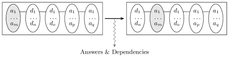
  Figure 9: Combining answers and dependencies in a local worklist.

Implementation Support

The key Prolog implementation support for these tables are mutable terms and non-backtrackable mutations (Appendix B). We also use a global variable for the table repository. These features are widely available. The non-backtrackable nature is essential to retain the collected answers and dependencies across disjunctions.

4.5 Completion of a Double Recursive Call

Example 4.6.

Consider a variant of our running example where the recursive clause is replaced by:

r(X,Y) :- r(X,Z), r(Z,Y).Figure 10 illustrates the computation of ?- r(a,Y). Each table is a rectangle. The consecutive states of its worklist are shown from top to bottom. A dotted arrow shows the target of a dependency. The solid and wavy lines are as in Figure 9. In the explanation, the labels of the completion steps in the figure are written between parentheses. The call ?- r(a,Y). gives rise to the dependency D1 = dependency(r(a,Z),r(Z,Y),r(a,Y)) and the answer r(a,b) (left rectangle).

Iteration 1

In the first iteration of completion (1), the answer is fed into the dependency (wavy arrow $\alpha$), hence D1 and r(a,b) are swapped. This exposes the call r(b,Y) (middle rectangle). For this new call we immediately obtain the dependency D2 = dependency(r(b,Z1),r(Z1,Y),r(b,Y)) and the answer r(b,c). We also record dependency D3 = dependency(r(b,Y),true,r(a,Y)) between r(b,Y) and r(a,Y). The true in D3 represents the empty continuation: finding an answer for r(b,Y) gives an answer for r(a,Y) for free!

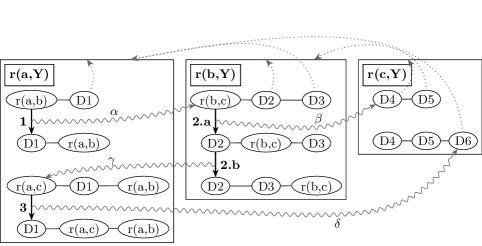
Figure 10: Illustration of the computation of r(a,Y).

Iteration 2

During the second iteration, we feed the answer r(b,c) into the two dependencies D2 (2.a, wavy arrow $\beta$) and D3 (2.b, wavy arrow $\gamma$).

1. In the D2 case, we expose a new call r(c,Y) (right rectangle) yielding no direct answer, but a new dependency D4 = dependency(r(c,Z2),r(Z2,Y),r(c,Y)) and a derived dependency D5 = dependency(r(c,Y),true,r(b,Y)).

2. In the D3 case, we obtain the new answer r(a,c) for the top-level call.

Iteration 3

During the third iteration (3), we feed the new answer into dependency D1 (wavy arrow $\delta$). This yields the call r(c,Y) and the dependency D6 = dependency(r(c,Y),true,r(a,Y)).

The fixpoint

Finally, there is no more work to be done: at the bottom of each rectangle, all D$i$ are left of all answers. Hence, the fixpoint comprises the answer table $\{\texttt{r(a,b)},\texttt{r(a,c)}\}$ for the call pattern r(a,Y), the answer table $\{\texttt{r(b,c)}\}$ for the call pattern r(b,Y) and the empty answer table for r(c,Y).

5 Evaluation

5.1 Implementation Effort

Table 1 summarizes the implementation effort in lines of Prolog (LoC). The control flow shown in this paper comprises 60 LoC, or less than 11% of the overall effort. The majority goes to the two kinds of data structures, the tries (40%) and the worklists (45%). Adding 25 lines of glue code, this amounts to an implementation for 577 Prolog LoC.

Category	LoC	Category	LoC
Control flow	60	Completion Worklists	259
Call and Answer Tries	233	Miscellaneous	25
Total	577

Table 1: Code size in lines of code.

5.2 Performance

While raw efficiency is not the main objective of our lightweight implementation, it is nevertheless important to achieve a reasonable performance compared to the existing state-of-the-art tabling systems. In order to evaluate this, we compare our implementation in hProlog 3.2.38 against XSB 3.4.0 [Swift and Warren (2012)], B-Prolog 8.1 [Zhou (2012)], Yap 6.3.4 [Santos Costa et al. (2012)] and Ciao 1.15-2731-g3749edd [Hermenegildo et al. (2012)] on a number of benchmarks. Table 2 summarizes the results (in ms) obtained on a Dell PowerEdge R410 server (2.4 GHz, 32 GB RAM) running Debian 7.6. In parentheses, we have indicated the maximum resident set size (RSS) in megabytes and the proportion of hProlog to XSB.

Discussion

The XSB system is the reference system for tabling; it has invested most time and resources in the development of its tabling infrastructure. We see that it is 8 to 38 times faster than our implementation, but 45 to 78 times faster for two outliers (path right last: binary tree 18 and 10k pingpong). It has a maximum RSS that is up to 7 times as large, and 14 times for path double first 500. In general, standard trie-based structures overload the memory because representation sharing is poor. This has been addressed by Raimundo and Rocha (?).

Since XSB does not support big integers, it was not meaningful to run the Fibonacci benchmark, recorded as O/F (for overflow). This is a case in point for wider tabling support in other systems: often we need both tabling and other non-standard features.

B-Prolog is only half as fast as XSB on many benchmarks, but is architecturally different: BProlog implements linear tabling and uses hash tables instead of tries. Moreover, in several cases B-Prolog is notably slower than XSB (i.e., n-reverse) and even much slower than our own implementation (recognize, shuttle, ping pong). Yet, unlike XSB, B-Prolog does support big integers and is substantially faster than our approach for the fib benchmark. All in all the results are mixed and point out several weaknesses in the B-Prolog implementation compared to our all Prolog implementation.

Benchmark	Size	hProlog	$\frac{\mathbf{hProlog}}{\mathbf{XSB}}$	$\frac{\mathbf{hProlog}}{\mathbf{B-Prolog}}$	$\frac{\mathbf{hProlog}}{\mathbf{Yap}}$	$\frac{\mathbf{hProlog}}{\mathbf{Ciao}}$
fiba	500	24 (13)	O/F (—)	$\infty$	$\infty$	—
	750	33 (13)	O/F (—)	17	41	—
	1,000	46 (13)	O/F (—)	46	19	—
	10,000	982 (66)	O/F (—)	3	44	—
recognizea	20,000	205 (73)	26 (1)	0.003	11	4
	50,000	503 (221)	30 (2)	0.001	14	4
n-reversea	500	767 (138)	38 (5)	11	15	45
	1,000	2,800 (537)	31 (6)	6	8	34
shuttleb	2,000	44 (12)	$\infty$ (2)	0.1	$\infty$	9
	5,000	138 (14)	23 (2)	0.08	$\infty$	12
	20,000	582 (29)	24 (4)	0.02	$\infty$	10
	50,000	1,586 (72)	29 (6)	0.01	$\infty$	12
ping pong	10,000	271 (16)	45 (2)	0.07	$\infty$	14
	20,000	490 (28)	35 (4)	0.03	$\infty$	8
path double first loop	50	653 (14)	19 (2)	13	$\infty$	7
	100	4,638 (29)	17 (4)	10	$\infty$	6
path double first	50	162 (12)	27 (2)	15	$\infty$	14
	100	989 (16)	20 (3)	12	$\infty$	10
	200	6,785 (53)	18 (7)	16	$\infty$	10
	500	110,463 (267)	25 (14)	19	$\infty$	14
path right last: pyramid 500	500	1,914 (104)	35 (7)	29	$\infty$	27
path right last: binary tree 18	18	108,662 (4,120)	78 (5)	50	3,461	42
test large joins 2c	12	3,001 (237)	10 (5)	4	$\infty$	12
joins mondial		6,444 (399)	8 (2)	7	224	6

Table 2: Results of the performance benchmarks.

Source: a [Fan and Dietrich (1992)]  b [Demoen and Sagonas (1998a)]  c Yap benchmark suite

The Yap tabling implementation, which is based on that of XSB, is clearly the fastest: the underlying engine is much faster [Rocha et al. (2000)]. It outperforms our approach on all benchmarks, and the other systems on most. Many benchmarks take less than $1\text{\,}\mathrm{ms}$, rounded down to $0\text{\,}\mathrm{ms}$, hence the factor $\infty$ in the table.

The performance of Ciao lies between that of XSB and B-Prolog. Performance of our implementation is within a factor 4 to 14 of Ciao, with reverse and path right last as outliers. Running the Fibonacci benchmarks is currently not possible, as tabling and bignums currently do not operate together.

Summary

We consider the performance results of our implementation very reasonable, especially if we take into account the stark contrast between our lightweight pure Prolog implementation and the complex integration in other systems. As part of future work, we think that advances in three areas may positively affect performance. Firstly, continuations are copied with copy_term/2. A special-purpose copy_continuation/2 could do better by exploiting the known structure of these terms. Other applications using delimited control could benefit from this optimization as well. Secondly, we don’t statically identify strongly connected components in the scheduling component. Doing so would allow the specialisation of completion. Finally, in contrast with state-of-the art implementations, our tries do not use substitution factoring.

6 Related Work

Delimited Control

While delimited control is well-known in the functional programming world, it has not received much attention in the context of Prolog. Only recently have Schrijvers et al. provided an unobtrusive implementation in the WAM  [Schrijvers et al. (2013), Schrijvers et al. (2013)]. In the continuation-passing implementation [Tarau and Dahl (1994)] of BinProlog [Tarau (2012)] this is even easier. Schrijvers et al. also illustrate the power of delimited control by porting various effect handlers [Plotkin and Pretnar (2013)] to Prolog. As far as we know, this paper shows the first Prolog-specific application.

XSB

XSB is the best-known Prolog engine supporting tabling. Its foundation, SLG resolution, has been described by Chen and Warren (?). Swift and Warren (?) provide a recent survey. Implementing XSB has required nontrivial changes to the architecture of the WAM. XSB maintains a forest of SLD-trees for a tabled predicate. During the computation, the stack may be frozen several times.

CAT and CHAT

The CAT is an alternative to the SLG-WAM used in XSB [Demoen and Sagonas (1998a)]. Rather than freezing memory areas, CAT uses incremental copies to preserve the execution state of suspended computations. CAT’s advantage is that the speed of the underlying abstract machine is not affected for non-tabled execution. CHAT is an improved scheme incorporating some ideas from the SLG-WAM [Demoen and Sagonas (1998b)]. CAT and CHAT do require changes to the WAM, but acknowledge that the complexity and scope of these changes should be kept limited.

Linear Tabling

Linear tabling mechanisms [Zhou et al. (2000)], which implement the SLDT-resolution strategy, maintain a single execution tree, hence there is the need to steal choicepoints from a former variant call. Each tabled call can be both a producer and a consumer. Similar to our approach, there is no overhead for standard SLD-resolution, but the need for recomputation of subgoals cannot always be avoided. Although simpler than SLG resolution, implementing SLDT still requires the addition of 4 new specifically designed WAM-instructions, a new frame structure and a new data area. Unlike for suspension-based mechanisms, the cut operator works for a class of useful programs.

DRA

The DRA [Guo and Gupta (2001), Guo and Gupta (2004)] has a goal similar to our approach. The technique implements tabled evaluation without stack-freezing. It postpones clauses containing variant calls at runtime, which is similar to our suspension creation. But to implement this technique, Guo and Gupta introduced six new WAM instructions. Compared to XSB, Guo and Gupta’s implementation of DRA has a significantly better space performance , but a worse time performance. The authors cite as sources for XSB’s better time performance that XSB avoids reconstructing the execution environment for applying looping alternatives, and secondly that XSB includes tabling in the compiling stage. Both reasons are equally applicable to our approach.

7 Conclusion

In order to enable a more widespread adoption of tabling, we have presented a lightweight implementation of tabling on top of delimited control. In contrast to existing approaches, our approach is implemented entirely in Prolog and requires no deep modifications to the WAM or complex program transformations. While there is obviously a trade-off between the simplicity of the implementation and runtime performance, we believe that the current performance of our approach is reasonable. Of course, there is ample opportunity for improvement.

In the future we would also like to extend our approach with mode-directed tabling [Guo and Gupta (2008), Santos and Rocha (2013)]. Our initial exploration has shown that this would only require a small change to the trie structure.

Acknowledgements

We are grateful to Bart Demoen for supporting hProlog and to the anonymous reviewers for their helpful feedback. This work was partly funded by the Flemish Fund for Scientific Research (FWO).

References

- Ceri et al. (1989) Ceri, S., Gottlob, G., and Tanca, L. 1989. What you always wanted to know about Datalog (and never dared to ask). IEEE Trans. on Knowl. and Data Eng. 1, 1, 146–166.
- Chen and Warren (1996) Chen, W. and Warren, D. S. 1996. Tabled evaluation with delaying for general logic programs. J. ACM 43, 1, 20–74.
- Danvy and Filinski (1990) Danvy, O. and Filinski, A. 1990. Abstracting control. In Proceedings of the 1990 ACM conference on LISP and functional programming. LFP ’90. ACM, 151–160.
- de Guzmán et al. (2008) de Guzmán, P. C., Carro, M., Hermenegildo, M. V., Silva, C., and Rocha, R. 2008. An improved continuation call-based implementation of tabling. In Practical Aspects of Declarative Languages, 10th International Symposium. Lecture Notes in Computer Science, vol. 4902. Springer, 197–213.
- Demoen and Sagonas (1998a) Demoen, B. and Sagonas, K. 1998a. Cat: The copying approach to tabling. In Principles of Declarative Programming, C. Palamidessi, H. Glaser, and K. Meinke, Eds. Lecture Notes in Computer Science, vol. 1490. Springer Berlin Heidelberg, 21–35.
- Demoen and Sagonas (1998b) Demoen, B. and Sagonas, K. 1998b. Chat: The copy-hybrid approach to tabling. In Practical Aspects of Declarative Languages, G. Gupta, Ed. Lecture Notes in Computer Science, vol. 1551. Springer Berlin Heidelberg, 106–121.
- Fan and Dietrich (1992) Fan, C. and Dietrich, S. W. 1992. Extension table built-ins for Prolog. Software: Practice and Experience 22, 7, 573–597.
- Felleisen (1988) Felleisen, M. 1988. The theory and practice of first-class prompts. In Proceedings of the 15th ACM SIGPLAN-SIGACT symposium on Principles of programming languages. POPL ’88. ACM, 180–190.
- Guo and Gupta (2008) Guo, H. and Gupta, G. 2008. Simplifying dynamic programming via mode-directed tabling. Softw., Pract. Exper. 38, 1, 75–94.
- Guo and Gupta (2001) Guo, H.-F. and Gupta, G. 2001. A simple scheme for implementing tabled logic programming systems based on dynamic reordering of alternatives. In Proceedings of ICLP’01. Springer, 181–196.
- Guo and Gupta (2004) Guo, H.-F. and Gupta, G. 2004. An efficient and flexible engine for computing fixed points. CoRR abs/cs/0412041.
- Hermenegildo et al. (2012) Hermenegildo, M. V., Bueno, F., Carro, M., Lípez-García, P., Mera, E., Morales, J. F., and Puebla, G. 2012. An overview of Ciao and its design philosophy. Theory Pract. Log. Program. 12, 1-2 (Jan.), 219–252.
- Plotkin and Pretnar (2013) Plotkin, G. D. and Pretnar, M. 2013. Handling algebraic effects. Logical Methods in Computer Science 9, 4.
- Raimundo and Rocha (2011) Raimundo, J. and Rocha, R. 2011. Global trie for subterms. Online Proceedings of the 11th International Colloquium on Implementation of Constraint Logic Programming Systems (CICLOPS 2011).
- Ramesh and Chen (1994) Ramesh, R. and Chen, W. 1994. A portable method for integrating SLG resolution into Prolog systems. In Proceedings of the 1994 International Symposium on Logic Programming. ILPS ’94. MIT Press, Cambridge, MA, USA, 618–632.
- Rocha et al. (2000) Rocha, R., Silva, F., and Santos Costa, V. 2000. YapTab: A tabling engine designed to support parallelism. In Conference on Tabulation in Parsing and Deduction. 77–87.
- Santos and Rocha (2013) Santos, J. and Rocha, R. 2013. On the efficient implementation of mode-directed tabling. In Practical Aspects of Declarative Languages - 15th International Symposium, PADL 2013. Lecture Notes in Computer Science, vol. 7752. Springer, 141–156.
- Santos Costa et al. (2012) Santos Costa, V., Rocha, R., and Damas, L. 2012. The YAP Prolog system. TPLP 12, 1-2, 5–34.
- Schrijvers et al. (2013) Schrijvers, T., Demoen, B., and Desouter, B. 2013. Delimited continuations in Prolog: Semantics, use and implementation in the WAM. Report CW 631, Dept. of Computer Science, KU Leuven.
- Schrijvers et al. (2013) Schrijvers, T., Demoen, B., Desouter, B., and Wielemaker, J. 2013. Delimited continuations for Prolog. Theory and Practice of Logic Programming (TPLP). Proceedings of the International Conference on Logic Programming (ICLP).
- Swift and Warren (2012) Swift, T. and Warren, D. S. 2012. XSB: Extending Prolog with tabled logic programming. Theory Pract. Log. Program. 12, 1-2 (Jan.), 157–187.
- Tarau (2012) Tarau, P. 2012. The BinProlog experience: Architecture and implementation choices for continuation passing Prolog and first-class logic engines. TPLP 12, 1-2, 97–126.
- Tarau and Dahl (1994) Tarau, P. and Dahl, V. 1994. Logic programming and logic grammars with first-order continuations. In LOPSTR ’94. Vol. 883.
- Zhou (2012) Zhou, N. 2012. The language features and architecture of B-Prolog. TPLP 12, 1-2, 189–218.
- Zhou et al. (2000) Zhou, N.-F., Shen, Y.-D., Yuan, L.-Y., and You, J.-H. 2000. Implementation of a linear tabling mechanism. In Practical Aspects of Declarative Languages, E. Pontelli and V. Santos Costa, Eds. Lecture Notes in Computer Science, vol. 1753. Springer Berlin Heidelberg, 109–123.