The Gaia-ESO Survey: Characterisation of the $\rm[\alpha/Fe]$ sequences in the Milky Way discs

Abstract

Context. High-resolution spectroscopic surveys of stars indicate that the Milky Way thin and thick discs follow different paths in the chemical space defined by $\rm[\alpha/Fe]$ vs $\rm[Fe/H]$, suggesting possibly different formation mechanisms for each of these structures.

Aims. We investigate, using the Gaia-ESO Survey internal Data-Release 2, the properties of the double sequence of the Milky Way discs (defined chemically as the high$-\alpha$ and low$-\alpha$ populations), and discuss their compatibility with discs defined by other means such as metallicity, kinematics or positions.

Methods. This investigation uses two different approaches: in velocity space for stars located in the extended Solar neighbourhood, and in chemical space for stars at different ranges of Galactocentric radii and heights from the Galactic mid-plane. The separation we find in velocity space allows us to investigate, in a novel manner, the extent in metallicity of each of the two sequences, identifying them with the two discs, without making any assumption about the shape of their metallicity distribution functions. Then, using the separation in chemical space, adopting the magnesium abundance as a tracer of the $\alpha-$elements, we characterise the spatial variation of the slopes of the $\rm[\alpha/Fe]-\rm[Fe/H]$ sequences for the thick and thin discs and the way in which the relative proportions of the two discs change across the Galaxy.

Results. We find that the thick disc, defined as the stars tracing the high$-\alpha$ sequence, extends up to super-solar metallicities ($\rm[Fe/H]\approx+0.2\,{\rm dex}$) and the thin disc, defined as the stars tracing the low$-\alpha$ sequence, at least down to $\rm[Fe/H]\approx-0.8\,{\rm dex}$, with hints pointing towards even lower values. Radial and vertical gradients in $\alpha-$abundances are found for the thin disc, with mild spatial variations in its $\rm[\alpha/Fe]-[Fe/H]$ paths, whereas for the thick disc we do not detect any such spatial variations, in agreement with results obtained recently from other high-resolution spectroscopic surveys.

Conclusions. The small variations in the spatial $\rm[\alpha/Fe]-[Fe/H]$ paths of the thin disc do not allow us to distinguish between formation models of this structure. On the other hand, the lack of radial gradients and $\rm[\alpha/Fe]-[Fe/H]$ variations for the thick disc indicate that the mechanism responsible for the mixing of the metals in the young Galaxy (e.g. radial stellar migration or turbulent gaseous disc) was more efficient before the (present) thin disc started forming.

1 Introduction

The decomposition and separation of the Galactic disc into thin and thick counter-parts, first suggested by Gilmore & Reid (1983), has many consequences in terms of Galaxy formation and evolution. Indeed, the differences in chemistry and kinematics between the stars of these two structures put constraints on both the role of mergers in the Galaxy in the last $8-12\,{\rm Gyr}$ (e.g.: Wyse, 2001; Abadi et al., 2003; Villalobos & Helmi, 2008) and on the importance of internal evolution mechanisms such as radial migration, dissipational cooling dependent on metallicity or clumpy turbulent discs (e.g.: Sellwood & Binney, 2002; Schönrich & Binney, 2009; Minchev et al., 2013; Bournaud et al., 2009).

Among the literature, there is no unique way of selecting stars belonging to either of the discs. Often, kinematic criteria are used, but selections based on chemical composition or spatial position are also employed, introducing potential biases in the distribution functions of the studied structures. Indeed, the first disc divisions, mainly based on star counts and density profiles, have found that the properties of the discs have an important overlap in kinematics and chemistry (Gilmore et al., 1989).

The advent of multi-object spectroscopy and large spectroscopic surveys such as SEGUE (Yanny et al., 2009) or RAVE (Steinmetz et al., 2006), confirmed these facts and measured the different kinematics relations of the discs (e.g. Nordström et al., 2004; Kordopatis et al., 2011, 2013c) and metallicities ([Fe/H]${}_{\rm thin}\leavevmode\nobreak\ \sim-0.1\,{\rm dex}$, [Fe/H]${}_{\rm thick}\leavevmode\nobreak\ \sim-0.5\,{\rm dex}$, e.g: Bensby et al., 2007; Reddy & Lambert, 2008; Ruchti et al., 2011; Kordopatis et al., 2013b). However, despite some specific attempts to characterise the wings of the distributions (e.g.: Norris et al., 1985; Chiba & Beers, 2000; Carollo et al., 2010; Ruchti et al., 2011; Kordopatis et al., 2013b, 2015) the overlap in kinematics and metallicity for the discs implies that the shape and extent of their distribution functions remain still quite uncertain. The best discriminant parameter seems to be the stellar age, the thick disc stars being consistently older than $9\,{\rm Gyr}$, (e.g.: Wyse & Gilmore, 1988; Edvardsson et al., 1993; Bensby et al., 2005; Bergemann et al., 2014; Haywood et al., 2013). Yet, stellar age is a parameter difficult to obtain, requiring either asteroseismic data, or parallax measurements combined with high-resolution spectroscopy.

In addition to age, the different formation histories of the two discs seems also strongly supported from the individual abundances measurements obtained for very local volumes of low mass FGK stars from very high-resolution spectra ($R\geq 35\,000$, e.g.: Fuhrmann, 1998, 2008, 2011; Reddy et al., 2006; Adibekyan et al., 2012; Bensby et al., 2014). In particular, the study of Bensby et al. (2014) used kinematic criteria to define the thin and thick discs, and found that each of these structures followed different sequences in the parameter space formed by the abundance ratio of $\alpha-$elements over the iron, as a function of iron $(\rm[\alpha/Fe]-\rm[Fe/H])$, with potentially a gap between these sequences. These results support previous conclusions that the thick disc stars were formed on a short time-scale, with relatively little pollution of the interstellar medium from supernovae of type Ia which are the main source of iron (e.g:. Wyse & Gilmore, 1988; Freeman & Bland-Hawthorn, 2002, and references therein).

All of the previously cited high-resolution surveys were, however, limited in volume (typically only probing up to $\sim 100\,{\rm pc}$ from the Sun) and often with complex selection functions combining metallicity and kinematics. Further high-resolution spectroscopic investigation was therefore needed in order to assess whether this separation was a global feature in the discs or a result of an observational bias. The gap could indeed disappear or become a trough farther away from the Sun, in which case the properties of the stars with intermediate $\alpha-$abundances would shed important light on the way the disc evolved chemically and dynamically.

Recio-Blanco et al. (2014) used the first data-release (iDR1) of the Gaia-ESO Survey (Gilmore et al., 2012), analysing faint FGK stellar populations with high resolution spectra ($R\sim 20\,000$) from the FLAMES/GIRAFFE spectrograph, to identify these two distinct sequences out to much larger volumes (up to distances of $5\,{\rm kpc}$ from the Sun) and made a first attempt to describe their chemo-dynamical characteristics. This analysis was pushed further by Mikolaitis et al. (2014), who derived, for the same observed dataset, abundances of eight elements (Mg, Al, Si, Ca, Ti, Fe, Cr, Ni, Y). Mikolaitis et al. (2014) concluded, consistent with other analyses, that the gap between the sequences is the most significant when considering the [Mg/Fe] abundance ratio as a function of [Fe/H], and that the two discs show no significant intrinsic dispersion in their $\alpha-$abundances at fixed [Fe/H]. This lack of scatter in the abundances along the metallicity for both thin and thick disc indicates first of all that the initial mass function (IMF) of the stars contributing to the $\rm[\alpha/Fe]$ ratio at low metallicities and the fraction of binary stars at the origin of supernovae type Ia, was constant over the formation time of the stars they pre-enrich, and in addition that the interstellar medium (ISM) should be very well mixed in order to have the same (small) dispersion at all metallicities.

Using only data for Red Clump stars from the Apache Point Observatory Galactic Evolution Experiment (APOGEE), Nidever et al. (2014) measured the $\rm[\alpha/Fe]-[Fe/H]$ trend for the thick disc and found that it had only very small variations with Galactocentric radius. Comparing with the results of a simple Galactic chemical evolution model, the authors concluded that the small amplitude, less than 10 per cent, of the spatial variations is possibly indicative of an essentially constant star formation efficiency, and constant outflow rate balancing the star-formation rate, during the early stages of the Milky Way while the stars that now form the thick disk were formed. Their favoured model has a star-formation efficiency corresponding to a gas consumption timescale of $2\,{\rm Gyr}$, close to that inferred for clumpy discs observed at redshift 2 (e.g. Tacconi et al., 2013).

We here use the FLAMES/GIRAFFE Gaia-ESO second internal data-release (iDR2) with its increased statistics (roughly a factor of two on the number of observed targets compared to iDR1), its enhanced analysis (use of a wider wavelength range in the spectral analysis due to an improvement of the parameter determination pipelines) and better quality (higher signal-to-noise ratio for the spectra, on average). We aim to characterise in a robust statistical way the chemical paths followed by the thin and thick discs, in velocity and space, in order to provide a thorough insight on its possible origins. The understanding of the chemical path origins will eventually further constrain disc formation theories, by indicating, for example, whether the thick disc was formed entirely in situ or by the contribution of extragalactic material (gas and/or stars).

Section 2 describes the dataset and the quality cuts that have been used in this work. Section 3 identifies in a novel manner the presence of the two disc populations by showing the way $\alpha-$abundances correlate with velocities. Section 4 identifies the two populations in terms of star-counts and investigates how their properties change at different Galactic regions. Finally, Sect. 6 summarises and concludes the present study. Note that in this paper we use the term metallicity to designate both the ratio of the global metal abundance to that of hydrogen ($\rm[M/H]$) and the ratio of the true iron abundance to that of hydrogen ($\rm[Fe/H]$). In general, the abundance pipeline for Gaia-ESO survey provides results such that $\rm[M/H]\approx\rm[Fe/H]$ (Recio-Blanco et al., in prep.), but we make explicit mention of one or the other parameter when confusion could occur.

Figure 1: Aitoff projection of the Galactic coordinates of the Gaia-ESO iDR2 targets used in this study.

2 Description of the data: Gaia-ESO iDR2

We use throughout this paper the parameters derived from spectra obtained with the FLAMES/GIRAFFE HR10 and HR21 settings (see Lewis et al., in preparation, for a description of the data reduction procedures). The Galactic coordinates $(\ell,b)$ of the observed targets are illustrated in Fig. 1. The source catalogue from which these targets are selected is the VISTA Hemisphere Survey (VHS, McMahon et al in prep.), with the primary selection being:

• $0.0<(J-K)<0.45$ for $14.0<J<17.5$

• $0.4<(J-K)<0.70$ for $12.5<J<15$.

Extinction was taken into account by shifting the colour-boxes by $0.5\times E(B-V)$, where $E(B-V)$ is the median Schlegel et al. (1998) extinction in that line-of-sight. If not enough targets were available within the colour cuts, additional targets were assigned by relaxing the red-edge of the colour-cut (see Gilmore et al., 2012, and Gilmore et al. in prep. for further details).

We adopted the recommended parameter values from the Gaia-ESO analysis for the effective temperature ($\rm T_{\rm eff}$), surface gravity ($\log g$) and elemental abundances and the iron abundance we use is derived from individual Fe I lines. The determination of the atmospheric parameters for the Gaia-ESO survey is described in Recio-Blanco et al. For the sake of completeness we give here a brief description of how these were obtained and refer the interested reader to the original reference for further details. We note that throughout the paper, the signal-to-noise ratio (S/N) refers to the value achieved in the HR10 setup (centred at $548.8\,{\rm nm}$). For a given star, the S/N in the HR21 setting (centred at $875.7\,{\rm nm}$) is approximately twice as large.

$\begin{array}[]{ccc}\includegraphics[width=143.09538pt,angle={0}]{R_Z_median_vr}&\includegraphics[width=143.09538pt,angle={0}]{R_Z_median_vphi}&\includegraphics[width=138.76157pt,angle={0}]{R_Z_median_vz}\end{array}$

Figure 2: Mean radial (left), azimuthal (middle) and vertical (right) Galactocentric velocities of the FLAMES/GIRAFFE stars in the Gaia-ESO internal Data-Release 2 (iDR2) as a function of their position in the Galaxy (in a cylindrical reference frame). For each panel, only the stars having errors less than $65\,{\rm km\,s^{-1}}$ in that particular component of space velocity are selected, resulting to 3162, 3667, 3243 targets, for $\rm V_{R}$, $\rm V_{\phi}$ and $\rm V_{Z}$ respectively. Mean values have been computed in bins of $0.4\,{\rm kpc}$ size, provided each position-bin contained at least 15 stars, resulting to an error on the mean velocity of $5\,{\rm km\,s^{-1}}$ per bin.

2.1 Determination of the atmospheric parameters and abundances

The stellar atmospheric parameters and abundances were determined by the members of the Gaia-ESO work package in charge of the GIRAFFE spectrum analysis for FGK-type stars. The individual spectra were analysed by three different procedures: MATISSE (Recio-Blanco et al., 2006), FERRE (Allende Prieto et al., 2006, and further developments) and Spectroscopy Made Easy (SME, Valenti & Piskunov, 1996, and further developments).

Each of these procedures performed well with respect to APOGEE results and well-studied open and globular clusters (i.e. the comparisons resulted in low-amplitude dispersions and simple biases). The random errors on the parameter values were reduced by putting the results from each procedure on the same scale, then combining them. This was achieved by first choosing the results of a given procedure as the reference, and then multi-linear transformations as a function of $\rm T_{\rm eff}$ and $\log g$ were used to put the results from the two other procedures on the same scale as the reference one. The adopted transformations were of the form:

$$\Delta\theta_{p}=\theta_{p}-\theta_{r}=c_{0}+c_{1}\cdot\mathrm{T}_{\mathrm{eff},p}+c_{2}\cdot\log g_{p}$$ (1)

where $\theta$ is one of $\rm T_{\rm eff}$, $\log g$, $\rm[M/H]$ or $\rm[\alpha/Fe]$, the subscript $r$ indicates the value from the reference procedure, and the subscript $p$ indicates the value from either of the other procedures (see Recio-Blanco et al., in prep., for more details).

The resulting random errors for each method were fairly similar ($\sim 60\,{\rm K}$ for $\rm T_{\rm eff}$, $0.14$ for $\log g$, $0.06$ for $\rm[M/H]$ and $0.05$ for $\rm[\alpha/Fe]$) and, as a consequence, the results for each star were combined by a simple average with the same weight given to each method. The averaged results were then calibrated with respect to 19 benchmarks stars (Jofré et al., 2014); this corrected for systematic biases of $+83$ K for $\rm T_{\rm eff}$ and $+0.23\,{\rm dex}$ for $\rm[M/H]$.

Once the final estimates of the values of the atmospheric parameters were obtained, the individual abundances, including the magnesium (Mg) and iron (Fe) abundances used in this work, were derived from three independent methods: an automated spectral synthesis method (Mikolaitis et al., 2014), a Gauss-Newton method using a pre-computed synthetic spectra grid (Guiglion et al., 2014) and SME (Valenti & Piskunov, 1996). In line with the Gaia-ESO consortium analysis, all the abundance analysis methods used MARCS (Gustafsson et al., 2008) model atmospheres. In addition, the input atomic and molecular data were provided by the linelist group of Gaia-ESO, who collated the most recent and complete experimental and theoretical data sources. The comparison of the results of each method showed that a simple shift was enough to put them all on the same scale. This shift was independent of both the atmospheric parameters and abundances, and corrected for small offsets with respect to the Solar abundance (of order $\pm 0.05\,{\rm dex}$). Finally, for each star and each element, the results of the three methods were averaged with equal weight, and the elemental abundances relative to the Sun (denoted [X/Fe] for element X) were obtained using the Grevesse et al. (2010) Solar elemental abundances.

The final mean (median) errors, corresponding to the parameter dispersion within the analysis nodes that have determined the atmospheric parameters and abundances are: $70\,{\rm K}$ ($36\,{\rm K}$) for $\rm T_{\rm eff}$, $0.14\,{\rm dex}$ ($0.08\,{\rm dex}$) for $\log g$, $0.08\,{\rm dex}$ ($0.06\,{\rm dex}$) for $\rm[Fe/H]$ and $0.06\,{\rm dex}$ ($0.05\,{\rm dex}$) for $\rm[Mg/Fe]$.

2.2 Determination of Galactocentric positions and velocities

The absolute magnitudes of the stars have been obtained by projecting the atmospheric parameters ($\rm T_{\rm eff}$, $\log g$, $\rm[M/H]$) and VISTA ${\rm(J-K_{s})}$ colour of the stars on the Yonsei-Yale isochrones (Demarque et al., 2004), as described in Kordopatis et al. (2011, 2013c), with the updates made in Recio-Blanco et al. (2014) concerning the treatment of the reddening. The derived distances have a mean uncertainty of 15 per cent. They were combined with the Galactic coordinates, line-of-sight velocities of the stars and the proper motions from the PPMXL catalogue (Roeser et al., 2010) in order to compute the Galactocentric positions and velocities in a cylindrical frame, with $\rm V_{R},\rm V_{\phi}$ and $\rm V_{Z}$ defined as positive with increasing $R,\phi$ and $Z$ (with the last towards the north Galactic pole). Typical errors of the proper motions are $4-10\,{\rm mas}\,{\rm yr^{-1}}$ (Roeser et al., 2010), resulting to transverse velocity errors at $2\,{\rm kpc}$ of $37-94\,{\rm km\,s^{-1}}$. The adopted Solar motion with respect to the Local Standard of Rest (LSR) is that of Schönrich et al. (2010), namely $\rm U_{\odot}=11.1,V_{\odot}=12.24,W_{\odot}=7.25\,{\rm km\,s^{-1}}$. Finally, the LSR is presumed to be on a circular orbit with azimuthal velocity $\rm V_{c}=220\,{\rm km\,s^{-1}}$, and we take the Sun to be located at $(\rm R_{0},Z_{0})=(8,0)\,{\rm kpc}$. The associated errors on the Galactocentric positions and velocities have been obtained by running 5000 Monte-Carlo realisations on the distances, proper motions and radial velocities and by measuring the dispersion of the derived parameters.

The mean stellar velocities (after the quality selections, see below) as a function of Galactocentric position are illustrated in Fig. 2, with a binning of $0.4\,{\rm kpc}$. The maps show consistent results with those already published in the literature. In particular, we detect a mild radial gradient in the velocity component along the radial direction $\rm V_{R}$, consistent with that found by Siebert et al. (2011b). This is visible at negative Z, going from $\sim 2\,{\rm km\,s^{-1}}$ at $R\sim 6.5\,{\rm kpc}$ to $\sim-5\,{\rm km\,s^{-1}}$ at $9\,{\rm kpc}$ ($\rm V_{R}$, left panel of Fig. 2). We also detect a compression/rarefaction pattern in the vertical velocity component, seen as the difference in sign of $<\rm V_{Z}>$ at $Z=\pm 1\,{\rm kpc}$ and $R=6,9\,{\rm kpc}$ (right panel, Fig. 2), consistent with the patterns identified in SEGUE G-dwarf data by Widrow et al. (2012) and in RAVE data by Williams et al. (2013) and Kordopatis et al. (2013b). These motions may be induced by external perturbations such as a satellite galaxy (e.g. Widrow et al., 2014) or internal perturbations such as spiral arms (e.g. Faure et al., 2014).

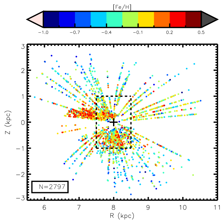
Figure 3: Scatter plot of the iron abundances of the stars having each of the components of their Galactocentric space velocity known better than $65\,{\rm km\,s^{-1}}$ as a function of their measured Galactocentric radius and distance from the plane. The position of the Sun, at $(R_{0},Z_{0})=(8,0)\,{\rm kpc}$, is indicated with a black ‘$+$’ symbol. The dashed box represent the selection made for the “local” sample around the Sun (see Sect. 3 and Sect. 4.4). Typical error on positions is 8 per cent.

2.3 Selection of subsamples based on quality cuts

The Gaia-ESO Survey observes three classes of targets in the Galaxy (field stars, members of open clusters and calibration standards, see Gilmore et al., 2012). Our analysis in this paper focuses on the Milky Way discs and therefore we kept only the field stars, i.e. those stars that are neither members of open clusters nor part of the calibration catalogue.

Furthermore, in order to have a dataset with reliable parameters, we excluded stars with spectra having a signal-to-noise ratio (S/N) less than 10 in the HR10 setup (higher S/N cuts have also been tested, without changing the overall conclusions of this paper) or having the highest uncertainties in the values of the derived parameters (i.e. being at the tails of the error distributions). As a compromise between accuracy and sample size, we set the cuts for the errors in effective temperature at $\sigma_{\rm T_{\rm eff}}\geq 250\,{\rm K}$ (4 per cent of the stars), in surface gravity at $\sigma_{\log g}\geq 0.5$ (3 per cent of the stars), in iron abundance at $\sigma_{\rm[Fe/H]}\geq 0.3\,{\rm dex}$ (0.5 per cent of the stars), and in line-of-sight distance at $\sigma_{D}/D\geq 0.5$ (4 per cent of the stars).

In addition, for each velocity component studied, we excluded those stars having errors in the given velocity greater than $65\,{\rm km\,s^{-1}}$. The errors in three-dimensional space velocity are dominated by the errors in the tangential velocities, so these rejection criteria lead to selection functions for each velocity component that are dependent on the stellar distances and the particular lines-of-sight (see Fig. 3). Indeed, stars close to the Galactic plane tend to have large errors on $\rm V_{Z}$, and stars towards the Galactic poles have poorly constrained $\rm V_{R}$. The removal of stars that had a derived error in a given velocity component that was greater than $65\,{\rm km\,s^{-1}}$, left us with 3162, 3667 and 3243 stars, for $\rm V_{R},\rm V_{\phi}$ and $\rm V_{Z}$, respectively. The spatial distribution of the 2797 stars that have errors in all three of their velocity components below $65\,{\rm km\,s^{-1}}$ is illustrated on Fig. 3, colour coded according to iron abundance. One can see from this plot that the metal-rich population ($\rm[Fe/H]>-0.2$ dex) is mostly found close to the plane, below $1\,{\rm kpc}$, as expected for a thin-disc dominated population.

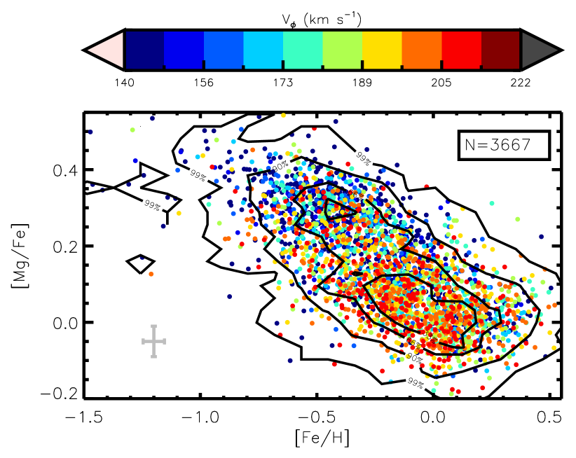
Figure 4: $\rm[Mg/Fe]$ as a function of $\rm[Fe/H]$ for the Gaia-ESO iDR2 stars with S/N$>10$. The mean error bar is represented in grey at the bottom left corner. The range of the plot has been truncated to $-1.5\leq\rm[Fe/H]\leq 0.55\,{\rm dex}$. The contour lines are drawn for 33 per cent, 66 per cent, 90 per cent and 99 per cent of the sample.

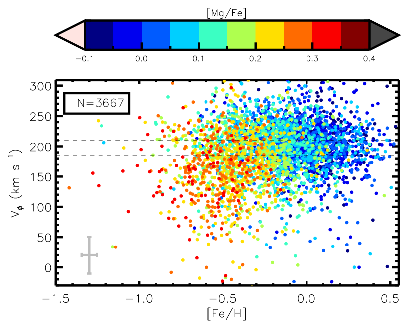
Figure 5: Azimuthal velocity as a function of $\rm[Fe/H]$, colour-coded according to the $\rm[Mg/Fe]$ abundance (the velocity and metallicity ranges have been truncated for visualisation purposes). Dashed horizontal lines are plotted at $\rm V_{\phi}=210\,{\rm km\,s^{-1}}$ and $\rm V_{\phi}=185\,{\rm km\,s^{-1}}$. Typical errors on $\rm V_{\phi}$ and $\rm[Fe/H]$ are represented at the bottom left corner, in grey.

Figure 4 shows the scatter plot of the azimuthal velocities of the 3667 stars that passed the error cut in this velocity component, in the chemical space defined by magnesium and iron. Following Mikolaitis et al. (2014), magnesium is used as the $\alpha-$element tracer in the remainder of this paper. The gap suggested from the analyses of Adibekyan et al. (2012, using the HARPS spectrograph), Bensby et al. (2014, using mainly the MIKE spectrograph) and Recio-Blanco et al. (2014, using the high S/N sample of Gaia-ESO iDR1) is seen in Fig. 4 as a trough, due to the low S/N threshold (S/N$>10$) we imposed for the analysis at this stage (median S/N$=25$; see Sect. 4.2 for an analysis of mock data illustrating how a real gap can get populated by noisy data and Sect. 4.4 for an analysis using higher S/N cuts on the Gaia-ESO iDR2 data). Indeed, the two populations - one low$-\alpha$ ($\rm[Mg/Fe]\lesssim 0.2\,{\rm dex}$) on orbits with higher azimuthal velocities (mean $\overline{\rm V_{\phi}}\sim 210\,{\rm km\,s^{-1}}$), and one high$-\alpha$ ($\rm[Mg/Fe]\gtrsim 0.1\,{\rm dex}$) on orbits with lower azimuthal velocities ($\overline{\rm V_{\phi}}\sim 185\,{\rm km\,s^{-1}}$) - can be identified with the colour-code. These two populations are more clearly seen in Fig. 5, representing $\rm V_{\phi}$ as a function of $\rm[Fe/H]$, colour-coded according to the $\rm[Mg/Fe]$ abundance. The fact that the high$-\alpha$ population has a larger velocity dispersion is also evident.

Given their different global kinematic properties, throughout this paper the high$-\alpha$ and low$-\alpha$ populations will be referred to as the thick and thin discs, respectively. In the next section, we explore the metallicity ranges up to which these two populations extend, by investigating their kinematics, but without decomposing the stellar populations.

3 The local disc dichotomy in terms of Galactocentric velocities

In this section we aim to investigate, for the stars in the greater Solar neighbourhood ($7.5\leq R\leq 8.5\,{\rm kpc}$ , $|Z|<1\,{\rm kpc}$) - the Solar suburbs - the metallicity range over which the disc(s) can be decomposed into at least two different populations, defined by their correlation between kinematics and chemical abundances. This we achieve with no a priori assumption about the shapes of their metallicity distribution functions (DF) or their kinematic DFs. Kinematics provide the means to discriminate among models for the formation and evolution of the discs, and the way in which metallicity and chemical abundances correlate with kinematics carries important and fundamental information on the nature of the stars in our sample (e.g. Eggen, Lynden-Bell, & Sandage, 1962; Freeman & Bland-Hawthorn, 2002; Rix & Bovy, 2013). For the remainder of this paper, we define a stellar population by demanding that its member stars show the same correlations between chemistry and kinematics over the whole range of metallicity that the population spans. The approach presented below is complementary to, and independent of, that of Sect. 4, where we fit the $\alpha-$abundances in different metallicity bins in order to trace the evolution of the trends for both discs, defined purely by chemistry.

3.1 The greater Solar neighbourhood sample

The disc stars in the greater Solar neighbourhood are selected by requiring distances close to the Galactic plane ($|Z|<1\,{\rm kpc}$), Galactocentric radii between $7.5$ and $8.5\,{\rm kpc}$ (i.e. distances from the Sun closer than $1.12\,{\rm kpc}$) and azimuthal velocities greater than $0\,{\rm km\,s^{-1}}$. These selections ensure that:

(i) The radial and vertical gradients in the discs have minimal effects on the interpretation of the results.

(ii) The sample under consideration is as homogeneous as possible towards all the lines-of-sight (see Fig. 3). Excluding stars farther than $1\,{\rm kpc}$ from the plane should not particularly bias the kinematics of the selected populations (other than the bias coming from possible vertical gradients in $\rm V_{\phi}$), provided that the populations are quasi-isothermal in vertical velocity dispersion, which appears to be a reasonable approximation (e.g.: Flynn et al., 2006; Binney, 2012; Binney et al., 2014).

(iii) The contamination by inner halo stars is reduced, in order to focus on the thin and thick disc chemical dichotomy. The adopted azimuthal velocity threshold of $0\,{\rm km\,s^{-1}}$ allows the retention of metal-weak thick disc stars, given an expected azimuthal velocity distribution for the thick disc that extends down to at least $60-80\,{\rm km\,s^{-1}}$ (i.e. $\sim\leavevmode\nobreak\ 0\,{\rm km\,s^{-1}}$ with a $65\,{\rm km\,s^{-1}}$ error, see Kordopatis et al., 2013b, c). This threshold simultaneously excludes counter-rotating stars likely to be members of the halo (in any case, the contribution from the halo should be small, given the metallicity range and distances above the plane investigated; see for example, Carollo et al., 2010). Note that in this work we treat the metal weak thick disc as part of the canonical thick disc; whether or not the chemo-dynamical characteristics of the metal-weak thick disc are distinct will be investigated in a future paper.

3.2 Description of the method

We assess the presence of two distinct populations in chemical space by measuring the mean velocities ($\mathrm{\overline{V_{i}}}$) and their dispersions ($\sigma_{V_{i}}$) for different $\rm[Fe/H]$ bins, in addition to the correlation(s) between the means of each of the velocity components and the stellar $\alpha-$enhancements (noted simply $\rm\partial V_{i}/\partial\rm[Mg/Fe]$). While the evolution of the mean velocities as a function of metallicity has long been used to identify the transition between the thin and thick discs (e.g.: Gilmore et al., 1989; Freeman & Bland-Hawthorn, 2002; Reddy et al., 2006), here the novel approach is to see whether there is a difference in the mean velocities at a given $\rm[Fe/H]$, as a function of $\rm[Mg/Fe]$. Non-zero values for $\rm\partial V_{i}/\partial\rm[Mg/Fe]$ can arise due to the following:

1. The estimated values of the atmospheric parameters, distances and velocities have correlated errors and therefore biases.

2. At least one population has a velocity gradient and/or chemical gradient as a function of Galactocentric radius and/or vertical distance, resulting in different kinematic properties in a given metallicity bin.

3. Only one population has an intrinsic correlation between chemistry and kinematics, as has previously been proposed for the thick disc in previous studies ($\partial\rm V_{\phi}/\partial\rm[Fe/H]\approx 50\,{\rm km\,s^{-1}}\,{\rm dex}^{-1}$, e.g: Kordopatis et al., 2011, 2013b).

4. There are at least two different populations with distinct kinematics and chemistry.

5. A combination of some or all of the above.

Possibility (1) is not likely. Indeed, as noted earlier (Sect. 2.1), the calibration using benchmark stars removed the known biases in the stellar parameters, while Recio-Blanco et al. (in prep.) found no significant degeneracies between the parameter determinations that could have led to artificial correlations between the parameters. Nevertheless, hidden biases may still exist. For example, a bias in metallicity, effective temperature or surface gravity could affect the final distance estimation and thus the final Galactocentric space velocity. Biases of less than $0.1\,{\rm dex}$ in $\rm[M/H]$ or less than $100\,{\rm K}$ in $\rm T_{\rm eff}$ (the maximum possible values for this analysis), could change the distances up to 10 per cent (see Schultheis et al., 2015, their Table 1, for further details). At $1\,{\rm kpc}$, this would translate to changes in velocities of $\sim 5\,{\rm km\,s^{-1}}$(assuming proper motions of $10\,{\rm mas}\,{\rm yr^{-1}}$), which is too small to have a significant effect on our analysis.

Concerning possibility (2), the amplitude of chemical gradients in the thin disc has been thoroughly discussed in the literature, with evidence from a variety of stellar tracers for mild radial and vertical metallicity gradients, of the order of $\partial\rm[Fe/H]/\partial R\approx-0.04$ to $-0.07\,{\rm dex}\,{\rm kpc}^{-1}$ and $\partial\rm[Fe/H]/\partial Z\approx-0.05$ to $-0.1\,{\rm dex}\,{\rm kpc}^{-1}$ (e.g. Gazzano et al., 2013; Boeche et al., 2013; Recio-Blanco et al., 2014; Anders et al., 2014). The thick disc shows no evidence for a radial metallicity gradient (e.g.: Cheng et al., 2012; Bergemann et al., 2014; Boeche et al., 2014; Mikolaitis et al., 2014) and at most a mild vertical metallicity gradient (Ruchti et al., 2010; Kordopatis et al., 2011, 2013c; Mikolaitis et al., 2014). The $\rm[\alpha/Fe]$ gradients in both discs are also small ($\lesssim\pm 0.02\,{\rm dex}\,{\rm kpc}^{-1}$), with the actual amplitude and even the sign being still a matter of debate (see Sect. 5 of Mikolaitis et al., 2014). As far as the kinematic trends are concerned, neither the radial gradient in $\overline{\rm V_{R}}$ ($\rm\partial\rm V_{R}/\partial R\approx 3\,{\rm km\,s^{-1}}\,{\rm kpc}^{-1}$, Siebert et al., 2011b) nor the “compression-rarefaction” patterns reported in $\overline{\rm V_{Z}}$ in both $\rm R$ and $\rm Z$ (Williams et al., 2013; Kordopatis et al., 2013a), are strong enough to contribute significantly within the volume of the greater Solar neighbourhood. A similar conclusion holds for $\overline{\rm V_{\phi}}$, given the studies of Lee et al. (2011) and Binney et al. (2014) based, respectively, on the SDSS-DR8 (Aihara et al., 2011) and RAVE-DR4 (Kordopatis et al., 2013a) catalogues for stars located roughly in the same volume as the present study.

The difference in the chemo-dynamical signature between that due to a single population having an intrinsic correlation between metallicity and kinematics, possibility (3) above, or that due to the superposition of several populations each with distinct correlations between metallicity and kinematics (possibility (4)) is more subtle. It can however be seen in the variation of the gradient of kinematics with chemistry, such as $\rm\partial V_{i}/\partial\rm[Mg/Fe]$ with metallicity. Indeed, a single population, as defined at the beginning of this section, should exhibit no trend in $\rm\partial V_{i}/\partial\rm[Mg/Fe]$ as a function of metallicity. A combination of more than one population would produce variations of this quantity if the relative proportions of the populations changes with $\rm[Fe/H]$. Our investigation of the extent of the superposition of the stellar populations using this approach therefore differs from those previously published in the literature, since here we make no assumptions about the number of these populations that may be present, nor the shape of their distribution functions (see for example Bovy et al., 2012b, for a decomposition of the disc into multiple mono-abundance populations).

Figure 6: Mean number of stars (A), Galactocentric radii (B), distances from the Galactic plane (C), azimuthal velocities (D), azimuthal velocity dispersions (E) as measured from the data (in black) and corrected by the error measurements (in green), at different metallicity bins, for stars located within the greater Solar neighbourhood. Panel F shows the correlations between the mean azimuthal velocity and the $\alpha-$abundance ratios for different metallicity bins. The error bars represent the $3\sigma$ Poisson noise averaged over the Monte-Carlo realisations. The bins are $0.07\,{\rm dex}$ wide, chosen as a compromise between the number of stars inside each bin and an adequate coverage of the metallicity range.

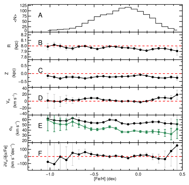
Figure 7: Same as Fig. 6 but for the radial velocity component, $\rm V_{R}$.

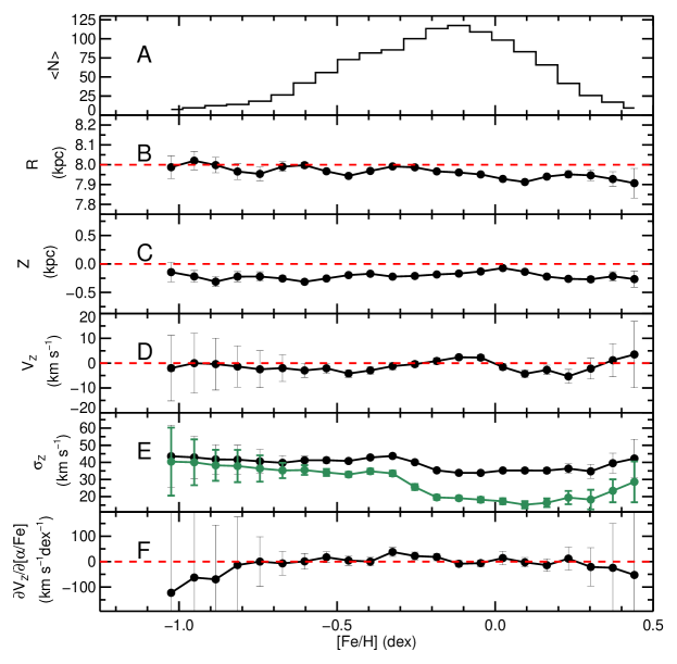
Figure 8: Same as Fig. 6 but for the vertical velocity component, $V_{Z}$.

Figures 6, 7, 8 and 9 show the results obtained for the azimuthal ($\rm V_{\phi}$), radial ($\rm V_{R}$) and vertical ($\rm V_{Z}$) velocity components of the stars. Each of these figures represent the mean number of stars per iron abundance bin (panels A), their mean radial distance from the Galactic centre (panels B), their distance from the plane (panels C), their mean velocity and dispersion (panels D and E), and finally the correlation between the mean velocity and the $\alpha-$abundances (panels F and Fig. 9). They have been obtained with 100 Monte-Carlo realisations on positions, velocities and iron abundance, and by keeping the iron bin boundaries at fixed values. Stars can therefore move between bins from one realisation to the next, as parameter values change with each realisation.

After each Monte-Carlo realisation, the mean velocities and $1\sigma$ velocity dispersions of the stars within each bin were measured, provided that bin contained at least 15 stars. As far as the $\rm\partial V_{i}/\partial\rm[Mg/Fe]$ values are concerned, they have been obtained by fitting a line in the $\rm V_{i}$ vs $\rm[Mg/Fe]$ parameter space and by measuring the slope of that line. The final values inside each bin were then obtained by computing the average over the realisations. The associated error bars were obtained by dividing the standard deviation of the means by the square root of the mean number of stars inside each bin. Finally, the corrected velocity dispersions (green lines in Figs. 6, 7 and 8) were obtained by removing quadratically two times the mean velocity error of the stars inside each bin, the factor of two arising since the errors are taken into account twice: first, intrinsic to the measurement, and then again during the Monte-Carlo realisations (see also Kordopatis et al., 2013b). We therefore used the following relation to correct the velocity dispersions for observational uncertainties:

$$\sigma_{V_{i}}=\sqrt{\sigma_{V_{i}}^{*2}-2\times mean(error_{V_{i}})^{2}}$$ (2)

where $\sigma_{V_{i}}$ represents the corrected velocity dispersion of $\rm V_{R},\rm V_{\phi}$ or $\rm V_{Z}$, and $\sigma^{*}_{V_{i}}$ is the corresponding measured velocity dispersion (averaged over the Monte-Carlo realisations). We refer the reader to Guiglion et al. (submitted) for a thorough analysis of the velocity dispersion of the disc stars as a function of the chemical composition.

3.3 Azimuthal velocity component

The identification of the thin and thick disc through the analysis of the stellar kinematics is most cleanly achieved using the azimuthal velocities of the stars, because of the asymmetric drift in the mean kinematics. Indeed, from the trends of the mean $\rm V_{\phi}$ velocity (Fig. 6, panel D), one can identify the thin disc component, with $\overline{\rm V_{\phi}}\sim 205\,{\rm km\,s^{-1}}$, dominating the star counts for metallicities above $-0.4\,{\rm dex}$. The thick disc, virtually unpolluted by the halo (due to the imposed cuts: $|Z|<1\,{\rm kpc}$ and $V_{\phi}>0\,{\rm km\,s^{-1}}$), is distinguishable below metallicities of $-0.5\,{\rm dex}$, where there is a decrease in the mean azimuthal velocities. The velocity dispersion (Fig. 6, panel E) at metallicities above $-0.2\,{\rm dex}$ has the value $\sigma_{\phi}\sim 25\,{\rm km\,s^{-1}}$. Below $-0.5\,{\rm dex}$, this increases to $\sigma_{\phi}\sim 45\,{\rm km\,s^{-1}}$. These values agree with the estimates of the velocity dispersions of the old thin and thick discs as measured far from the Solar neighbourhood (Kordopatis et al., 2011), those measured for stars in the RAVE survey within roughly the same volume (Binney et al., 2014), and other values available from the literature (e.g.: Soubiran et al., 2003; Lee et al., 2011).

As far as the correlations between $\rm V_{\phi}$ and $\rm[\alpha/Fe]$ are concerned, (Fig. 6, panel F and Fig. 9, top plot), the behaviour of $\partial\rm V_{\phi}/\partial\rm[Mg/Fe]$ with increasing metallicity shows three regimes:

• a value close to zero at super-solar metallicities,

• a non-zero value of $\partial\rm V_{\phi}/\partial\rm[Mg/Fe]\approx-120\,{\rm km\,s^{-1}}\,{\rm dex}^{-1}$ below $-0.5\,{\rm dex}$, compatible with little variation within the errors,

• an intermediate regime between metallicities $[-0.5,+0.2]\,{\rm dex}$, where the amplitude of $\partial\rm V_{\phi}/\partial\rm[Mg/Fe]$ monotonically increases with metallicity. We interpret this variation as indicative of a varying mixture of populations.

We note that these trends are not depending on the adopted binning in metallicity, since they are also recovered when adopting, for example, overlapping bins $0.07\,{\rm dex}$ wide, spaced by $0.05\,{\rm dex}$. Following from the discussion at the beginning of Sect. 3, these three regimes suggest that the relative proportions of the different stellar populations present in our sample do not vary significantly above $+0.2\,{\rm dex}$, since we find no trend of $\partial\rm V_{\phi}/\partial\rm[Mg/Fe]$ with metallicity in this range. Similar conclusions can be made below $-0.5\,{\rm dex}$, although the larger error bars in this regime could hide weak trends. In terms of separate thin and thick discs, the trends we find imply that the metallicity distribution of the thick disc extends at least up to Solar values, and that of the thin disc goes down to at least $-0.5\,{\rm dex}$. This overlap in metallicity was already suggested from the $\alpha-$abundance trends derived from very-high resolution studies of stars in the immediate Solar neighbourhood ($d<100\,{\rm pc}$, e.g. Reddy et al., 2006; Adibekyan et al., 2013; Bensby et al., 2014; Nissen, 2015), and by Nidever et al. (2014) for stars in a wide range of Galactic radii ($0\lesssim R\lesssim 15\,{\rm kpc}$).

We can further assess the presence of thin disc stars below $\rm[Fe/H]=-0.5\,{\rm dex}$ by making a rough separation of the stars within a given $\rm[Fe/H]$ bin into either high$-\alpha$ ($\rm[Mg/Fe]>0.3\,{\rm dex}$) or low$-\alpha$ ($\rm[Mg/Fe]<0.2\,{\rm dex}$, see also Sect. 5.1) candidates. This results in the low$-\alpha$ population having a median $\rm V_{\phi}\sim 212\,{\rm km\,s^{-1}}$, whereas the median $\rm V_{\phi}$ of the high$-\alpha$ population is $\sim 165\,{\rm km\,s^{-1}}$. The low$-\alpha$ population has a lag compared to the LSR that is typical of the thin disc, and the lag for the high$-\alpha$ population is consistent with estimates for the canonical and metal weak thick disc, provided there is a correlation between $\rm V_{\phi}$ and $\rm[Fe/H]$ of $50\,{\rm km\,s^{-1}}\,{\rm dex}^{-1}$, as found by Kordopatis et al. (2013a). We therefore conclude that the thin disc metallicity distribution extends down to at least $\rm[Fe/H]=-0.8\,{\rm dex}$. Below that metallicity, the number of stars is too small to allow us to derive a reliable estimate of the mean velocity. The relative proportion of thin disc stars at low metallicities will be discussed further in Sect. 4.

A natural outcome of the existence of thin disc stars below $\rm[Fe/H]<-0.5\,{\rm dex}$ is that the non-zero $\partial\rm V_{\phi}/\partial\rm[Mg/Fe]$ value that we measure is at least partly due to the mixture of thin and thick disc. However, within the errors, Fig. 9 shows a flat behaviour below $\rm[Fe/H]\lesssim-0.5\,{\rm dex}$, suggesting a constant fraction of thick/thin disc. This result will also be found when separating the stars according to their $\alpha-$abundances. Indeed, while we cannot eliminate the possibility that there exists an intrinsic correlation between $\rm V_{\phi}$ and $\rm[\alpha/Fe]$ for the thick disc stars, as suggested by Recio-Blanco et al. (2014), we note that the differences that we find in the median $\rm V_{\phi}$ values for $\rm[Mg/Fe]\sim 0.35\,{\rm dex}$ and $\rm[Mg/Fe]\sim 0.1\,{\rm dex}$ ($165\,{\rm km\,s^{-1}}$ and $212\,{\rm km\,s^{-1}}$, respectively), could be sufficient to explain the measured value of $\partial\rm V_{\phi}/\partial\rm[Mg/Fe]\approx-120\,{\rm km\,s^{-1}}\,{\rm dex}^{-1}$, provided a fixed fraction of thick disc stars over thin disc stars of approximately 60 per cent. This ratio is in good agreement with the local thin disc / thick disc ratio of 3:2 for the metallicity bin $[-0.8,-0.6]$ derived by Wyse & Gilmore (1995) through the combination of a volume-complete local sample ($d\lesssim 30\,{\rm pc}$) and an in situ sample at $Z\sim 1\,{\rm kpc}$ (after scaling with appropriate density laws and kinematics).

3.4 Radial and vertical velocity components

Due to the fact that both the radial and vertical velocity distribution functions are centred at zero for both discs, the thin/thick disc dichotomy is harder to identify with these velocity components. The investigation of the mean velocities as a function of metallicity confirms indeed this fact (see panel D of Fig. 7 and Fig. 8), where we find mean velocities centred around $0\,{\rm km\,s^{-1}}$.

The velocity dispersions (panels E) of the most metal-poor stars are found to be $(\sigma_{R},\sigma_{Z})\approx(50,40)\,{\rm km\,s^{-1}}$, typical of thick disc values, while the most metal-rich stars have dispersions more typical of the thin disc, being $(\sigma_{R},\sigma_{Z})\approx(30,20)\,{\rm km\,s^{-1}}$ (e.g.: Soubiran et al., 2003; Lee et al., 2011; Bovy et al., 2012a; Sharma et al., 2014). In particular, the abrupt change in the slope $\partial\sigma_{Z}/\partial\rm[Fe/H]$ for metallicities $\gtrsim-0.4\,{\rm dex}$ suggests that this is the metallicity threshold above which the thin disc becomes the dominant population. This point will be confirmed in Sect. 4.4, where the discs are separated in chemical space only.

As far as the $\rm\partial V_{R,Z}/\partial\rm[Mg/Fe]$ trends are concerned, we find them being consistent with zero at least within the metallicity range $[-0.8,+0.2]\,{\rm dex}$. The results using $\rm V_{\phi}$ showed that the relative proportion of the populations is changing across this metallicity range. Therefore, the invariant, null value for $\rm\partial V_{R,Z}/\partial\rm[Mg/Fe]$ implies that all populations present in our sample share common radial and vertical velocity distributions, at least in the mean.

An investigation of the detailed trends of the velocity dispersions is outside the scope of this paper, but we did investigate the specific case of the behaviour of $\partial\sigma_{Z}/\partial\rm[Mg/Fe]$ as a function of metallicity, as this may be compared with the independent analysis of Guiglion et al. (2015, submitted). We find a non-zero value for the metal-poor stars (though still marginally compatible with zero at the 3$\sigma$ level). This value, suggests that in a given metallicity range the thick disc stars have a larger velocity dispersion than the thin disc ones (i.e. the low$-\alpha$ ones), as expected (see Guiglion et al. for details).

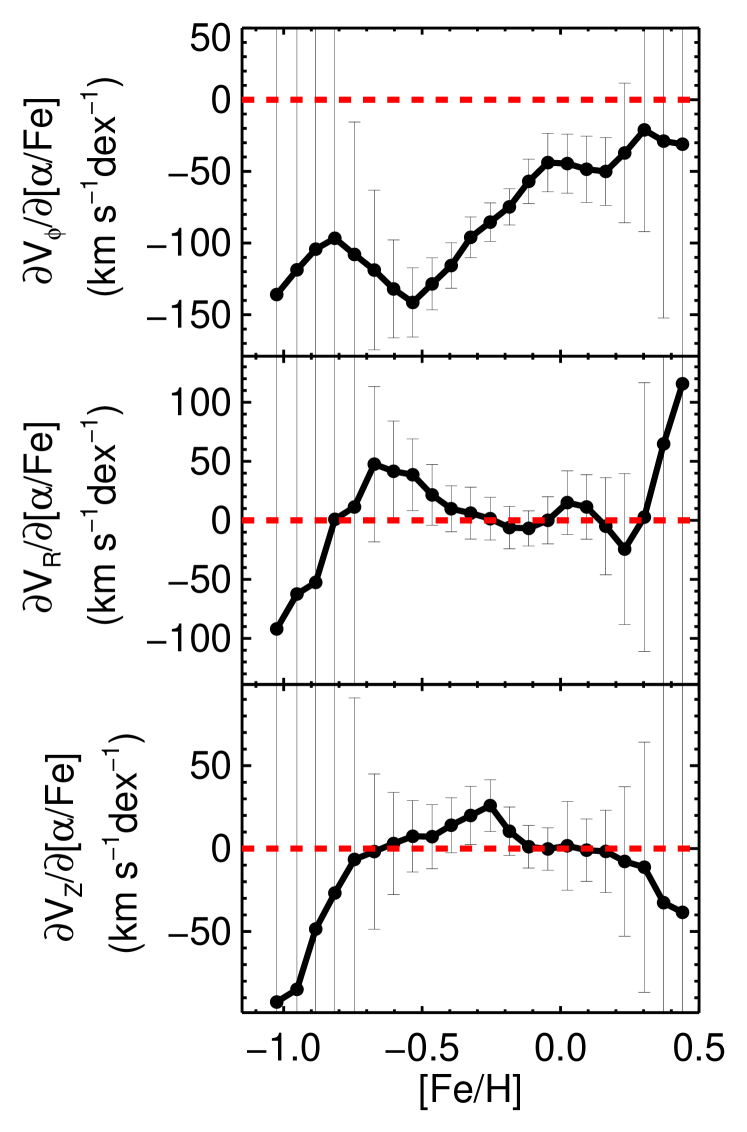
Figure 9: Same as panels F of Figs. 6 to 8, but put side by side to facilitate comparison of the trends. The plots have been smoothed with a boxcar average taking into account the closest neighbour.

3.5 Discussion

Our analysis of the mean azimuthal velocities of the stars shows that for metallicities between $-0.8$ and $+0.2\,{\rm dex}$, there is a mixture of at least two populations in our sample. Further, their relative proportions vary with metallicity. This is a well-established result for the thin and thick disks defined by kinematics (e.g. Carney et al., 1989; Wyse & Gilmore, 1995; Bensby et al., 2005, 2007); the new result here refers to the discs when defined by distinct chemical abundance patterns.

Our results show that the thin disc, defined as the low$-\alpha$ population, extends in metallicity at least as low as $-0.8\,{\rm dex}$, whereas the thick disc, defined as the high$-\alpha$ population, extends at least up to Solar metallicities. Outside the $[-0.8,+0.2]\,{\rm dex}$ range, the large error bars that we derive in our analysis cannot allow to draw any robust conclusions.

The metallicity ranges over which we have found the discs to extend have to be considered in light of the results of Haywood et al. (2013) and Snaith et al. (2014). These authors concluded that chemical evolution was traced by the thick disk up to high metallicities, then after dilution by metal-poor gas, proceeded following the thin disk sequence from low metallicity to high metallicity. A thick disc extending up to super-Solar metallicities plus a thin disc extending down to $-0.8\,{\rm dex}$, challenge this view since such a large metallicity overlap - over $1\,{\rm dex}$ - would require accretion of a significant mass of metal-poor gas to lower the ISM’s metallicity before the onset of star formation in the thin disc. We note, however, that we have not corrected for the selection function in our analysis. Further, we have very limited information concerning stellar ages.

Future data from Gaia will provide better age estimates from improved distances and absolute magnitudes, in addition to proper motions that are ten times more accurate than those we adopted here, which will allow a more refined analysis.

4 Identification and characterisation of the $\rm[Mg/Fe]$ sequences in terms of star-counts

In the previous section we identified and confirmed the existence of two populations in our Solar suburb sample, for metallicities between $[-0.8,+0.2]\,{\rm dex}$. In that analysis we made no assumptions about the underlying metallicity distribution functions. In this section, we extend the analysis to an investigation of the $\alpha-$abundance sequences across the entire metallicity range of the data. We aim to characterise the possible double structure in each metallicity bin, and obtain estimates of the mean $\alpha-$enhancement value, and the dispersion, of each component, for different regions of the Galaxy (i.e. both within and beyond the extended Solar neighbourhood). As in the previous sections, we use the magnesium abundance as a tracer of the $\alpha-$abundance of the stars, and we make the reasonable assumption that at a fixed $\rm[Fe/H]$ the Gaia-ESO survey is not biased with respect to the value of $\rm[Mg/Fe]$.

4.1 Model fitting of the data

The model-fitting is done using a truncated-Newton method (Dembo & Steihaug, 1983) on the un-binned $\rm[Mg/Fe]$ data of a given metallicity range, by maximising the log-likelihood of the following relation:

$$\mathcal{L}(\mu_{1},\sigma_{1},\rho_{1},\mu_{2},\sigma_{2},\rho_{2})=\prod_{t=1}^{N}\sum_{i=1}^{2}\frac{\rho_{i}}{\sqrt{2\pi\sigma_{i}^{2}}}\cdot e^{-\frac{(\rm[\alpha/Fe]_{t}-\mu_{i})^{2}}{2\sigma_{i}^{2}}}$$ (3)

where $N$ is the total number of stars considered in a given metallicity range, $\mu_{1},\mu_{2},$ are the mean $\rm[\alpha/Fe]$ values of the thin and thick disc, $\sigma_{1},\sigma_{2}$ are the dispersions on the $\rm[\alpha/Fe]$ abundances, $\rho_{1}$ and $\rho_{2}$ are the relative proportions of each population, and $\rm[\alpha/Fe]_{t}$ is the $\rm[\alpha/Fe]$ abundance ratio of a given star measured from its spectrum. The fit is performed for every Monte-Carlo realisation separately.

Motivated by the results of Adibekyan et al. (2013); Bensby et al. (2014); Recio-Blanco et al. (2014), we assume that the mean $\rm[\alpha/Fe]$ abundance of each population with $\rm[Fe/H]\geq-0.9\,{\rm dex}$ is a function of metallicity, and that the thin disc’s mean $\rm[\alpha/Fe]$ at any metallicity is always lower than (or equal to) the mean $\rm[\alpha/Fe]$ abundance of the thick disc. We note that the thick disc exhibits an $\rm[\alpha/Fe]$ plateau at lower metallicities (e.g. Ruchti et al., 2010), this plateau ending with the so-called knee of the $\rm[\alpha/Fe]-\rm[Fe/H]$ distribution. The exact position of the knee is a matter of debate; its location depends on how quickly star formation and chemical enrichment happened in the thick disc. The quality of our data at the lowest metallicities does not, however, allow us to investigate this issue.

To perform our fitting, the initial assumed values for the mean $\alpha-$enhancements of the discs are:

$$\mu_{\rm thick} = -0.30\times{\rm[Fe/H]}+0.2$$ (4)

$$\mu_{\rm thin} = -0.10\times{\rm[Fe/H]}.$$ (5)

We allow the fitting procedure to vary these means freely by up to $\pm 0.15\,{\rm dex}$. As far as the dispersions of the distributions are concerned, we allow them to vary in the interval between $[0.05,0.15]\,{\rm dex}$, and start with an initial value of $0.08\,{\rm dex}$, larger than the typical errors in $\rm[\alpha/Fe]$ (see Sect. 2.1).

This set of assumptions allows the value of $\rm[Mg/Fe]$ at the low metallicity end of the thick disc distribution to be between $0.35$ and $0.65\,{\rm dex}$ (consistent with the results of Mikolaitis et al., 2014, obtained with the Gaia-ESO DR1 dataset). Furthermore, the priors also ensure that the thin disc sequence has enhancements that are close to Solar values at Solar metallicities and that the $\rm[Mg/Fe]$ prior for the thick disc is always higher than that for the thin disc (the starting relations are equal at ten times the solar iron abundance).

Note that our procedure always fits two components to the data, even in regions where only one sequence could exist. Since a model with two components will always fit the data better, we investigate the significance of this fit by deriving the $p-$value of the log-likelihood ratio between the null hypothesis of having only one thick/thin disc and the alternative model of having both components. We therefore define the following test statistic of three degrees of freedom:

$$D=2\cdot\left(\log\mathcal{L}_{2}-\log\mathcal{L}_{1}\right)$$ (6)

where $\mathcal{L}_{2}$ is the likelihood associated to the model with two components (5 degrees of freedom, see Eq. 3) and $\mathcal{L}_{1}$ is the likelihood associated to the null model with only one component (2 degrees of freedom). We set that for a given Monte-Carlo realisation the two components model is the more likely if $D\geq 7.82$, which corresponds to a $p-$value $\leq 0.05$. We then derive the mean fitted populations over all the Monte-Carlo realisations, and conclude that two populations are needed only if the mean is greater than 1.5 (i.e. the two component model is preferred for more than half of the realisations with 0.95 confidence).

This procedure has been applied to six subsamples, selected by location within the Galaxy: three ranges in Galactocentric radius (inner Galactic ring: $6.5-7.5\,{\rm kpc}$, Solar suburbs: $7.5-8.5\,{\rm kpc}$, outer Galactic ring: $8.5-10\,{\rm kpc}$), and two distances from the plane ($|Z|<1\,{\rm kpc}$ and $1<|Z|<2\,{\rm kpc}$). The results, obtained after averaging 100 Monte-Carlo realisations on distances, metallicities and $\rm[Mg/Fe]$ abundances, are discussed in the following sections.

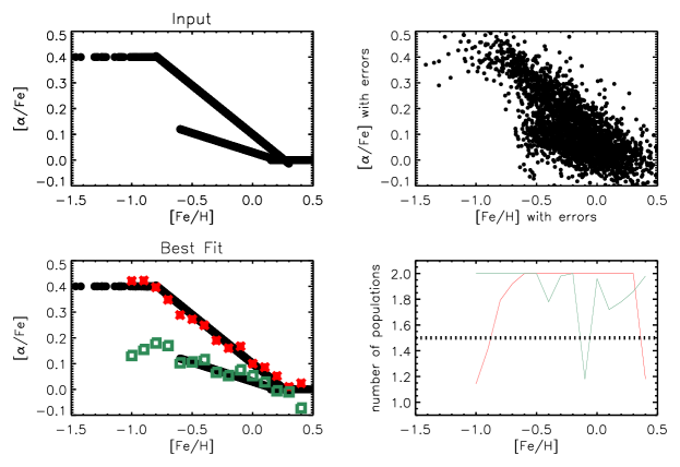
Figure 10: Top: adopted trends for the mock data used to test our fitting procedure (left) and effect on the mock data of introducing errors in $\rm[Fe/H]$ and $\rm[\alpha/Fe]$ as the observations (right). Bottom: Output of our fitting procedure for the high$-\alpha$ (red crosses) and low$-\alpha$ (green squares) populations performed on the noisy mock data. Over-plotted in black are the error-free points used to create the mock catalogue. The bottom right plot shows the average of the number of populations needed to better fit the data based on the log-likelihood ratio tests of Eq. 6. When the red (green) line is below $1.5$, this indicates that fitting the data with only a thick (thin) disc rather than two components simultaneously is more significant for more than half of the Monte-Carlo realisations.

4.2 Tests on mock data

We tested our fitting procedure on mock data to verify that it is able to find the “correct” $\alpha-$enhancements of two populations with chemical trends similar to what is expected in the Milky Way. For that purpose, we took the $\rm[Fe/H]$ values of the stars in our sample, and assigned for the range $-0.8<\rm[Fe/H]<+0.3$ the trends seen on the top left plot of Fig. 10: the position of the thick disc knee is located at $-0.8\,{\rm dex}$, the thin disc’s lowest metallicity is $-0.6$, and the two sequences merge at $\rm[Fe/H]\geq 0.3$. These values are selected in order to roughly represent the actual data, while still differing from the priors of Eqs. 4 and 5; this should allow us to verify that our procedure converges towards the correct results. The ‘stars’ were randomly assigned to either the high$-\alpha$ or low$-\alpha$ population. Then, for each ‘star’ we assigned the uncertainties of the true Gaia-ESO iDR2 catalogue, to reproduce realistic error bars. The blurring due to the uncertainties on the iron and $\alpha-$abundances can be seen in the top-right panel. One can notice that the underlying gap in the chemical paths is now barely visible and that Fig. 10 is qualitatively similar to Fig. 4 where the actual Gaia-ESO data are plotted.

We applied our procedure, starting from equations (4) and (5), to 100 Monte-Carlo realisations of noisy mock data and derived the average trends plotted in red crosses and green square symbols on the bottom left panel of Fig. 10. One can see that the “true” trends are nicely recovered, up to Solar metallicities, validating our procedure. In particular, the procedure performs well for a gap-width varying with metallicity, even when the separation is very small. Our procedure also correctly finds that at the low metallicities a single high$-\alpha$ population is enough to fit the data. Indeed, despite fitting two populations even at the lowest metallicities (green squares below $\rm[Fe/H]=-0.6$ in the lower left panel of Fig. 10), the relative weight associated to these points, combined with the test statistic of Eq. 6, indicate that these points are not likely to represent correctly the data (the red line in the bottom right plot of Fig. 10 is consistently below 1.5).

The difficulty of fitting the data towards the highest metallicities, where the the separation between the two sequences is small, can be seen on the noisiness of the average log-likelihood ratio, comparing the two-component model with a model having only the thin disc (green line). We note, however, that the two component model is always the preferred fit, even at this regime, as it should be, based on the input mock data.

In the following sub-sections, we therefore apply our procedure with confidence to the Gaia-ESO iDR2 data.

4.3 Robustness to signal-to-noise cuts

Figure 11 shows the trends of the high$-\alpha$ and low$-\alpha$ populations at different Galactocentric radii and distances from the plane, colour-coded according to different cuts in S/N of the actual Gaia-ESO spectra. One can see that our results are robust to these cuts, with the overall trends being similar, independent of the S/N threshold. Lowering the threshold increases the number of analysed stars and populates regions of chemical space which statistically have fewer stars, i.e. at lower and higher metallicities. A lower S/N threshold therefore achieves a better description of the overall behaviour of the trends, but with larger uncertainties on individual estimates, particularly at the extremes of the metallicities. In the remainder of this analysis, when not stated otherwise, we adopt S/N$>25$ as providing a compromise between the number of analysed stars and the errors on the trends. All the quality cuts on distance and atmospheric parameter errors remain similar to the ones of Sect. 2.3.

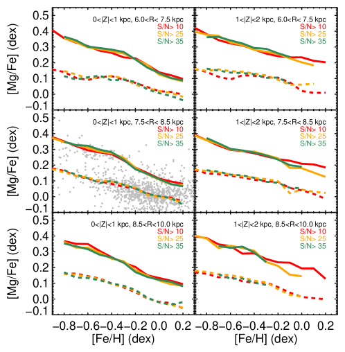
Figure 11: Trends of the $\rm[Mg/Fe]-\rm[Fe/H]$ sequences for the thick disc (plain line) and thin disc (dashed line), for different signal-to-noise (S/N) threshold limits close to the plane ($0<|Z|<1\,{\rm kpc}$, left column) and far from it ($1<|Z|<2\,{\rm kpc}$, right column). The top, middle and bottom rows show the Gaia-ESO iDR2 results for the inner Galaxy, Solar suburb and outer Galaxy, respectively. The over-plotted grey points in the panel $7.5<R<8.5\,{\rm kpc}$ and $0<|Z|<1\,{\rm kpc}$ are the $\alpha-$abundance measurements of Adibekyan et al. (2013), obtained for a very local sample ($d\lesssim 150\,{\rm pc}$). No significant differences in the derived trends are found as a function of S/N, which is indicative of the robustness of our fitting method.

$\begin{array}[]{ccc}\includegraphics[width=212.47617pt,angle={0}]{Scatter_plot_afe_vs_Feh_Solar_cylinder_Z_lt1_SNR10}&\includegraphics[width=212.47617pt,angle={0}]{Scatter_plot_afe_vs_Feh_Solar_cylinder_Z_gt1_SNR10}\\ \includegraphics[width=212.47617pt,angle={0}]{Scatter_plot_afe_vs_Feh_Solar_cylinder_Z_lt1_SNR25}&\includegraphics[width=212.47617pt,angle={0}]{Scatter_plot_afe_vs_Feh_Solar_cylinder_Z_gt1_SNR25}\\ \includegraphics[width=212.47617pt,angle={0}]{Scatter_plot_afe_vs_Feh_Solar_cylinder_Z_lt1_SNR35}&\includegraphics[width=212.47617pt,angle={0}]{Scatter_plot_afe_vs_Feh_Solar_cylinder_Z_gt1_SNR35}\end{array}$

Figure 12: $\rm[Mg/Fe]$ as a function of $\rm[Fe/H]$ for the stars in the Solar neighbourhood, closer than $1\,{\rm kpc}$ from the Galactic plane (left panels) and between $1\,{\rm kpc}$ and $2\,{\rm kpc}$ from the plane (right panels). Different selections, according to the signal-to-noise ratio of the spectra, are shown at the top (S/N$>10$) and the bottom (S/N $>35$). The colour-code corresponds to the azimuthal velocity of the stars. The dashed blue (black) line corresponds to the best fit model of the thick (thin) disc. The black ‘+’ sign is located at $\rm[Mg/Fe]=0$ and $\rm[Fe/H]=0\,{\rm dex}$.

4.4 Properties within $7.5<R<8.5\,{\rm kpc}$

We start by describing our results in the Solar suburbs ($7.5\leq R\leq 8.5\,{\rm kpc}$) at two different height-bins from the Galactic plane: $|Z|<1\,{\rm kpc}$ and $1<|Z|<2\,{\rm kpc}$. Figure 12 shows the matching of the recovered trends with the data-points at different S/N cuts, Fig. 13 represents the $\rm[Mg/Fe]$ dispersions as a function of $\rm[Fe/H]$, and finally middle plots of Fig. 14 and Fig. 15 show the derived relative numbers of the two sequences close and far from the plane, and the mean required populations to fit the data. For both heights, the two populations are recovered nicely, with no particular indication of a merging of the sequences up to $\rm[Fe/H]\approx+0.2$. Indeed, the mean number of populations above $\rm[Fe/H]>0$ (second column of Fig. 15) is most of the time greater than or close to 1.5, however with a noisy and decreasing trend indicating the difficulty of fitting robustly our data.

As mentioned in the previous Section, the data do not allow us to recover reliably the position of a ‘knee’ in the $\rm[\alpha/Fe]$ trend. However, we do recover the slopes of the decrease of the $\rm[Mg/Fe]-\rm[Fe/H]$ for each of the low$-\alpha$ and high$-\alpha$ sequences. These slopes depend on the histories of star formation and gas accretion/outflow (e.g.: Snaith et al., 2014; Nidever et al., 2014, see also Sect. 5). The measured slopes are reported in Table 4 and are discussed in the following subsections.

4.4.1 Close to the plane

For the stars close to the plane, in the metallicity interval $[-0.9,0.0]\,{\rm dex}$ we find (see Table 4):

$$\mu_{\rm thin} = (-0.20\pm 0.04)\times{\rm[Fe/H]}+(0.00\pm 0.02)$$ (7)

$$\mu_{\rm thick} = (-0.31\pm 0.05)\times{\rm[Fe/H]}+(0.12\pm 0.02)$$ (8)

Table 1: Slopes of the $\rm[Mg/Fe]-\rm[Fe/H]$ relations for thin and thick disc stars obtained for S/N$\geq 25$.

		$|Z|(\,{\rm kpc})<1$		$1<|Z|(\,{\rm kpc})<2$
		$a$	$b$	$a$	$b$
	$R(\,{\rm kpc})\leq 7.5$	$-0.14\pm 0.07$	$0.03\pm 0.04$	$-0.16\pm 0.04$	$0.06\pm 0.02$
Thin disc	7.5$<R(\,{\rm kpc})\leq 8.5$	$-0.20\pm 0.04$	$0.00\pm 0.02$	$-0.17\pm 0.05$	$0.04\pm 0.02$
	$R(\,{\rm kpc})>8.5$	$-0.23\pm 0.03$	$0.00\pm 0.02$	$-0.14\pm 0.08$	$0.03\pm 0.04$
	$R(\,{\rm kpc})\leq 7.5$	$-0.27\pm 0.05$	$0.14\pm 0.02$	$-0.25\pm 0.05$	$0.19\pm 0.02$
Thick disc	7.5$<R(\,{\rm kpc})\leq 8.5$	$-0.31\pm 0.05$	$0.12\pm 0.02$	$-0.21\pm 0.05$	$0.19\pm 0.02$
	$R(\,{\rm kpc})>8.5$	$-0.28\pm 0.07$	$0.13\pm 0.03$	$-0.19\pm 0.15$	$0.14\pm 0.07$

These slopes are robust to different S/N cuts (see Fig. 11; note we adopted S/N$>25$), and are found to fit well the trends of Adibekyan et al. (2013) (grey points in Fig. 11, in the panel representing the Solar suburb). In addition, we found that increasing the S/N threshold emphasises the gap between the two chemical sequences by depopulating the region between the chemical sequences (see Fig. 12). The prominence of this gap is therefore compatible with the results of Bensby et al. (2014); Recio-Blanco et al. (2014), we note, however, that in order to establish whether this gap is true or just a trough, depopulated due to low number statistics, additional data will be needed (e.g. the future data-releases of Gaia-ESO).

Our results show a steeper slope for the $\rm[Mg/Fe]$ sequence of the thick disc compared to the thin disc. As we will discuss in the following sections, a steeper slope implies higher ratio of past to present SFR (provided there is a fixed stellar IMF and Type Ia supernova delay distribution function for both discs). Above Solar metallicities (where the determination of the slope is not performed), we notice a flattening of the sequence for the thin disc (see Fig. 12) that could be compared to the “banana shape” quoted in Nidever et al. (2014, their Fig. 10), also seen in Bensby et al. (2014, their Fig. 15).

We find that the $\alpha-$enhancement dispersion, i.e. the thickness of the chemical sequence followed by either one of the discs, is of the order of $\sigma_{\rm[Mg/Fe]_{thin}}\sim 0.08\,{\rm dex}$ and $\sigma_{\rm[Mg/Fe]_{thick}}\sim 0.07\,{\rm dex}$, in agreement with Mikolaitis et al. (2014), obtained using the Gaia-ESO iDR1. We note, however, that below $\rm[Fe/H]\lesssim-0.7\,{\rm dex}$, the thin disc dispersion increases to $0.1\,{\rm dex}$; this is due to low number statistics, as our test on the significance of the fit indicates that below this metallicity, one component model is on average a better fit to the data.

$\begin{array}[]{cc}\includegraphics[width=216.81pt,angle={0}]{disp_trends_Solar_cylinder_Z_lt1_SNR20}&\includegraphics[width=216.81pt,angle={0}]{disp_trends_Solar_cylinder_Z_gt1_SNR20}\end{array}$

Figure 13: $\rm[Mg/Fe]$ dispersions as a function of $\rm[Fe/H]$, for the thick disc stars (in black) and the thin disc stars (in blue), close to the Galactic plane (left) and far from it (right).

$\begin{array}[]{ccc}\includegraphics[width=143.09538pt,angle={0}]{prop_trends_Inner_cylinder_Z_lt1_SNR20}&\includegraphics[width=143.09538pt,angle={0}]{prop_trends_Solar_cylinder_Z_lt1_SNR20}&\includegraphics[width=143.09538pt,angle={0}]{prop_trends_Outer_cylinder_Z_lt1_SNR20}\\ \includegraphics[width=143.09538pt,angle={0}]{prop_trends_Inner_cylinder_Z_gt1_SNR20}&\includegraphics[width=143.09538pt,angle={0}]{prop_trends_Solar_cylinder_Z_gt1_SNR20}&\includegraphics[width=143.09538pt,angle={0}]{prop_trends_Outer_cylinder_Z_gt1_SNR20}\end{array}$

Figure 14: Relative proportion of the high$-\alpha$ (in black) and low$-\alpha$ (in blue) populations as a function of $\rm[Fe/H]$, for increasing Galactocentric radii (from left to right) and distances from the Galactic plane (upper panels: close to the plane, lower panels: far from the plane). Plain thick lines represent measurements derived from observations, smoothed with a boxcar average taking into account the closest neighbour, whereas thin red and grey lines are derived from the toy model described in Table 2, with the scale-heights and scale-lengths of Jurić et al. (2008) and Bovy et al. (2012b), respectively.

$\begin{array}[]{ccc}\includegraphics[width=143.09538pt,angle={0}]{chi2_Inner_cylinder_Z_lt1_SNR20}&\includegraphics[width=143.09538pt,angle={0}]{chi2_Solar_cylinder_Z_lt1_SNR20}&\includegraphics[width=143.09538pt,angle={0}]{chi2_Outer_cylinder_Z_lt1_SNR20}\\ \includegraphics[width=143.09538pt,angle={0}]{chi2_Inner_cylinder_Z_gt1_SNR20}&\includegraphics[width=143.09538pt,angle={0}]{chi2_Solar_cylinder_Z_gt1_SNR20}&\includegraphics[width=143.09538pt,angle={0}]{chi2_Outer_cylinder_Z_gt1_SNR20}\end{array}$

Figure 15: Number of required populations, averaged over 100 Monte-Carlo realisations, as a function of metallicity. For each realisation, the significance of the $\chi^{2}-$distribution is evaluated, and the likelihood of requiring one or two populations is evaluated. Blue (black) line represents the results for the low$-\alpha$ (high$-\alpha$) population. A value larger than 1.5 indicates that the low$-\alpha$ (high$-\alpha$) population cannot describe by itself the observed trends.

For the considered local sample, the relative proportion of the low$-\alpha$ over high$-\alpha$ stars varies from 30 per cent to 80 per cent in the iron abundance range between $[-0.8,0.0]\,{\rm dex}$, reaching 50 per cent at [Fe/H]$\sim-0.4\,{\rm dex}$ (middle plots of Fig. 14). Below $\rm[Fe/H]\sim-0.5\,{\rm dex}$, we find that the proportion of thin disc to thick disc stars is slowly decreasing down to $\rm[Fe/H]\approx-0.8\,{\rm dex}$. This result is in agreement with the analysis of Sect. 3.3, where we investigated the change in the relative proportions of the different stellar populations by analysing the variations in $\partial\rm V_{\phi}/\partial\rm[Mg/Fe]$. Indeed, recall that in Sect. 3.3 we found that below $-0.5\,{\rm dex}$, and at least down to $-0.8\,{\rm dex}$, the value of $\partial\rm V_{\phi}/\partial\rm[Mg/Fe]$ varied only slowly as a function of metallicity (albeit with large error bars) which is consistent with only a small variation in the relative number of stars of each disc within this metallicity range. This therefore also implies that the shape of the metallicity distribution functions of the discs are significantly non-Gaussian (see also Hayden et al., 2015). We note that these results are robust to S/N selections and should not be dependent of the selection function, assuming there is no bias in $\rm[\alpha/Fe]$ at fixed $\rm[Fe/H]$. For the most metal-poor bin ($\rm[Fe/H]=-0.9\,{\rm dex}$), we find that the proportion of the low$-\alpha$ stars increases up to 45 per cent. Combined with the significance of the fit, and the increase of the $\rm[Mg/Fe]$ dispersion (see above), this indicates that this increase is not real, and is rather due to low number statistics.

Finally, we notice that both sequences are seen at all the metallicities, from $-0.8\,{\rm dex}$ up to super-Solar values. However, the fact that the relative proportion trend reverses for $\rm[Fe/H]\gtrsim 0.1$ (middle-top panel of Fig. 14) suggests that the number of stars in these bins is too small to perform a robust likelihood estimation and therefore separating the two populations when the sequences merge is challenging (as already mentioned in Sect. 4.3). This is also indicated from the plot of Fig. 15, where the significance of having only a thin disc rather than two populations (blue line), is noisy above solar metallicities.

We now assess to what extent the derived proportions are in agreement with the expected metallicity and spatial distribution functions of the discs. To do so, we model the expected number, N, of stars of a given disc as a function of Galactocentric radius, $R$, distance from the mid-plane, $Z$, and metallicity, $\rm[Fe/H]$, as:

$$N(R,Z,{\rm[Fe/H]})=f\cdot\exp{\left[-\frac{Z}{h_{Z}}-\frac{R-R_{0}}{h_{R}}\right]}\cdot{\rm MDF},$$ (9)

where $f$ is the local density of stars belonging to each of the discs, and ($h_{Z}$,$h_{R}$) are the scale-height and scale-length. The MDF is the adopted metallicity distribution function, defined as:

$${\rm MDF}=\sum_{i=1}^{3}a_{i}\cdot\\ \exp\left[-\frac{({\rm[Fe/H]}-M_{i})^{2}}{2\sigma_{i}^{2}}\right].$$ (10)

It is obtained as the sum of three Gaussians, associated with the metal-poor, intermediate metallicity, and metal-rich regimes, in order to reproduce skewed distributions. The factor $a_{i}$ is the weight assigned to each of these metallicity regimes, while $M_{i}$ and $\sigma_{i}$ are the mean metallicity and dispersion of the associated Gaussian. We assume that the MDF has a fixed shape, but can shift to lower or higher mean metallicities as a function of $R$ and $Z$. We therefore define $M_{i}$, as follows:

$$M_{i}=\mu_{i}+Z\cdot\partial\rm[Fe/H]/\partial Z+(R-R_{0})\cdot\partial\rm[Fe/H]/\partial R,$$ (11)

where $R$ is expressed in kiloparsecs and $\mu_{i}$ is the mean of the metal-poor, intermediate and metal-rich regimes, as measured at the Solar neighbourhood. The input values for our simple expectation models are summarised in Tables 2 and 3.

The adapted parameters are not chosen in order to fit the Gaia-ESO data, but are a compilation derived from the literature, based on discs defined either by kinematics, chemical abundance or star-counts. Therefore, the parameters of Table 2 roughly reproduce the skewness of the MDFs for the metal-weak regime of the thin and thick discs (Wyse & Gilmore, 1995; Kordopatis et al., 2013b) and the super-solar metallicity stellar distribution of RAVE (Kordopatis et al., 2015). The vertical and radial metallicity gradients of the thin disc are adopted from Mikolaitis et al. (2014) and Gazzano et al. (2013), respectively. Finally we adopt the scale-heights and scale-lengths of Jurić et al. (2008, defined morphologically) and Bovy et al. (2012b, defined chemically, see their Tables 1 and 2), to illustrate how the star counts are expected to change when considering a thick disc that is more extended or less extended than the thin disc.

Table 2: Input values for the metallicity distribution functions of the discs.

	thin disc	thick disc
$f$	0.85	0.14
$a_{1}(\,{\rm dex})$	0.90	0.80
$\mu_{1}(\,{\rm dex})$	0.0	$-0.5$
$\sigma_{1}(\,{\rm dex})$	0.08	0.35
$a_{2}(\,{\rm dex})$	0.1	0.15
$\mu_{2}(\,{\rm dex})$	$-0.3$	$-0.8$
$\sigma_{2}(\,{\rm dex})$	0.3	0.5
$a_{3}(\,{\rm dex})$	0.02	0.05
$\mu_{3}(\,{\rm dex})$	$+0.2$	$+0.2$
$\sigma_{3}(\,{\rm dex})$	0.5	0.5
$\partial\rm[Fe/H]/\partial R\leavevmode\nobreak\ (\,{\rm dex}\,{\rm kpc}^{-1})$	$-0.05$	0.00
$\partial\rm[Fe/H]/\partial Z\leavevmode\nobreak\ (\,{\rm dex}\,{\rm kpc}^{-1})$	$-0.06$	0.00

Table 3: Adopted scale-lengths and scale-heights of the discs.

	Thin disc		Thick disc
	$h_{R}$	$h_{Z}$	$h_{R}$	$h_{Z}$
	$(\,{\rm kpc})$	$(\,{\rm kpc})$	$(\,{\rm kpc})$	$(\,{\rm kpc})$
Jurić et al. (2008)	2.6	0.30	3.6	0.9
Bovy et al. (2012b)	3.8	0.27	2.0	0.7

The expected proportions of thin and thick discs are plotted in Fig. 14. One can see that for the sample in the range $7.5<R<8.5\,{\rm kpc}$, close to the plane (middle top panel), the expected trends are not matching correctly the observed ones: the model of Jurić et al. (2008) over- (under-) estimates the thick (thin) disc relative proportions, whereas the inverse is noticed for the Bovy et al. (2012b) model. We note, however, that modifying the Bovy et al. (2012b) model, with a thin disc slightly more compact ($h_{R}=3.6\,{\rm kpc},h_{Z}=0.25\,{\rm kpc}$) and a thick disc with a larger scale-height ($h_{Z}=0.9\,{\rm kpc}$), gives a trend in a better agreement with the observations.

4.4.2 Far from the plane

For the stars being between 1 and $2\,{\rm kpc}$ from the Galactic plane (bottom plots of Figs. 12 to 15), we find that the slopes of the mean $\alpha-$abundances are slightly flatter, compared to the derived values closer to the plane ($\mu_{\rm thin}=(-0.17\pm 0.05)\times\rm[Fe/H]+0.04$, $\mu_{\rm thick}=(-0.21\pm 0.05)\times\rm[Fe/H]+0.19$). In addition, the mean $\alpha-$enhancement of the discs at a given metallicity is increased by $\sim 0.04\,{\rm dex}$ for the thin disc and $\sim 0.07\,{\rm dex}$ for the thick disc (Fig. 17), in agreement with the vertical $\rm[\alpha/Fe]$ gradients in the discs found by Mikolaitis et al. (2014).

In addition, despite the fact that the selection function of Gaia-ESO is not taken into account (see Sect. 2), we find that the relative weight of the two populations changes, with the relative importance of the thick disc being higher, as expected (e.g.: Minchev et al., 2014). At Solar metallicities, at these heights above the plane, the thick disc represents 50 per cent of the stars. Compared to our star-count models, the agreement with the Bovy et al. (2012b) model is very good, in particular for the metal-poor part ($\rm[Fe/H]\lesssim-0.4$), however with again an over-estimation of the thin disc relative proportion at the higher metallicities.

Finally, the $\rm[\alpha/Fe]$ dispersions show mild trends (Fig. 13): the thick disc’s one decreases from $0.07\,{\rm dex}$ at low metallicities to $0.05\,{\rm dex}$ at super-solar values, as does the thin disc’s, with however an important increase for metallicities below $-0.6\,{\rm dex}$. Nevertheless, this increase is only due to the low number of stars available to fit for the low$-\alpha$ sequence, as shown by the relative proportion in Fig. 14 and the significance of the fit for metallicities below $\rm[Fe/H]\sim-0.6\,{\rm dex}$ (Fig. 15).

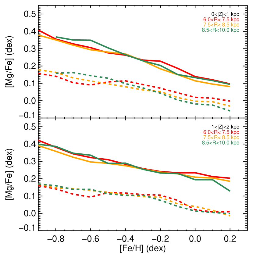
Figure 16: Trends at different Galactocentric radii for given bins of distances from the Galactic plane. Plain and dashed lines are associated to the high$-\alpha$ and low$-\alpha$ populations, respectively.

4.5 Investigation beyond $7.5<R<8.5\,{\rm kpc}$

The same fitting procedure as for the Solar suburbs has been repeated for radii intervals between $6.0<R<7.5\,{\rm kpc}$ and $8.5<R<10.0\,{\rm kpc}$. The bin sizes are purposely wider than the ones at the Solar suburb, in order to have enough stars to analyse, and in order to minimise the impact of having an inhomogeneous sky coverage (see Fig. 3). Figure 14 shows how the relative proportion of each population changes as a function of the region in the Galaxy. One can see that the proportion of the thick disc decreases with $R$, both close and far from the plane, suggesting that the thick disc is more radially concentrated than the thin disc, in agreement with previous surveys (e.g.: Bensby et al., 2011; Cheng et al., 2012; Bovy et al., 2012b; Anders et al., 2014; Recio-Blanco et al., 2014; Mikolaitis et al., 2014), and that the metal-weak tail of the low$-\alpha$ population does not extend below $-0.6$ in the $6.5<R<7.5\,{\rm kpc}$ ring. Our star-count models achieve a fitting of the relative proportions in different ways: for the range $6.0<R<7.5\,{\rm kpc}$, the model of Jurić et al. (2008) (thick disc longer than the thin disc) seems more appropriate, however, the Bovy et al. (2012b) model, which is assuming a shorter scale-length for the thick disc, is in better agreement for the stars located at the largest radii. This disagreement could indicate a varying scale-length or scale-height with $R$ for either or both of the discs, as recently suggested by Minchev et al. (2015).

The $\rm[Mg/Fe]-\rm[Fe/H]$ slopes as a function of $\rm[Fe/H]$ at the three Galactic regions are shown in Fig. 16, and summarised in Table 4. Overall we find that as a function of $R$, the thick disc has similar trends, whereas the thin disc slopes become marginally steeper (from $-0.14\pm 0.07$ at $R\leq 7.5\,{\rm kpc}$ to $-0.23\pm 0.03$ at $R\geq 8.5\,{\rm kpc}$). In addition the slopes become, on average, flatter as a function of $Z$, by $0.03\pm 0.05$ for the thin disc and by $0.07\pm 0.04$ for the thick disc.

The result from the Gaia-ESO survey obtained here, that the high-$\alpha$ thick disc sequence varies little spatially, is consistent with the conclusions from the APOGEE data for red clump stars published recently by Nidever et al. (2014). Those authors found that the overall spatial variations of the $\rm[\alpha/Fe]-\rm[Fe/H]$ sequence of the high$-\alpha$ stars do not exceed 10 per cent.

Finally, we find that the mean $\alpha-$enhancement for both discs are increased higher from the plane, at all Galactocentric radii. This is indicative of a vertical gradient in $\alpha-$elements in the thin disc, in agreement with the value of $+0.04\,{\rm dex}\,{\rm kpc}^{-1}$ measured in Mikolaitis et al. (2014).

Figure 17: Trends at different distances from the Galactic plane: $6<R<7.5\,{\rm kpc}$ (top), $7.5<R<8.5\,{\rm kpc}$ (middle) and $8.5<R<10\,{\rm kpc}$ (lower panel).

5 Discussion: Implications for how the discs evolved

The steepness of the $\rm[\alpha/Fe]-\rm[Fe/H]$ slopes contains information about how discs have evolved, encoding mainly information on the time evolution of their Star Formation Rates (SFR) and gas in/out flows, assumed to regulate the SFR. Typically, the $\rm[\alpha/Fe]$ decline with increasing $\rm[Fe/H]$ is caused by the time delay distribution that the first supernovae of type Ia (mostly iron producers) have after the core-collapse supernovae (mainly producers of $\alpha-$elements). After the adoption of an IMF, binary fraction and delay time distribution, the relative present to past SFR can be translated into a relative rate of core-collapse to Type Ia supernovae. In turn, this defines a slope of $\rm[\alpha/Fe]-[Fe/H]$ for the ISM and hence for newly formed stars, modulo possible elemental-dependent gas in/out flows.

In the case that most of the stars are formed during a starburst event, followed by a negligible star formation, then the slope of the decline – tracing the abundance of the gas – is maximal: the $\rm[\alpha/Fe]-[Fe/H]$ slope connects the last star formed before the end of the starburst and the first one to form after the gas has been enriched by SNIa ejecta. On the other hand, flatter slopes, i.e. slower declines, imply more important contributions from massive stars through core-collapse supernovae and thus more extended star formation. A typical slope for a closed-box star-forming system with a slowly decreasing SFR as inferred for the solar neighbourhood and standard Type Ia delay time distribution is around $-0.3$ (see e.g. Fig. 1 of Gilmore & Wyse, 1991). The flattening of the slope as the star-formation efficiency (defined as the reciprocal of the duration of star formation) decreases is illustrated in the top panel of Fig. 15 of Nidever et al. (2014). The middle panel of that figure in Nidever et al. (2014) illustrates how changing the rate of gas outflow can also change the slope.

Our work finds steeper slopes for the thick disc ($\approx-0.28\times\rm[Fe/H]$) compared to the thin disc, with negligible spatial variations as a function of $R$ and $Z$. On the other hand, the thin disc slopes show a variation as a function of $R$, with the flatter slope being in the inner Galaxy ($-0.14\times\rm[Fe/H]$) and the steeper in the outer Galaxy ($-0.23\times\rm[Fe/H]$).

Edvardsson et al. (1993) undertook a pioneering study of kinematics and elemental abundances, for a sample of 189 F and G dwarfs observed at the solar neighbourhood. They investigated the manner in which the $\rm[\alpha/Fe]$ abundance of a star in a given bin of $\rm[Fe/H]$ depends on the star’s mean orbital radius, using this as a proxy for birth radius. These authors found that stars from the outer Galaxy (mean orbital radius $R_{m}\geq 9\,{\rm kpc}$) follow an $\rm[\alpha/Fe]-\rm[Fe/H]$ relation that falls slightly below that followed by stars with mean orbital radius close to the Solar Circle. Further, they found that for stars from the inner Galaxy ($R_{m}\leq 7\,{\rm kpc}$), the $\rm[\alpha/Fe]$ values split into two groups: one at $\rm[\alpha/Fe]=0.2\,{\rm dex}$ for $\rm[Fe/H]<-0.4\,{\rm dex}$, and one at $\rm[\alpha/Fe]=0.03\,{\rm dex}$ for $\rm[Fe/H]\geq-0.4\,{\rm dex}$. The conclusion of their analysis was that the variation of the $\rm[\alpha/Fe]-\rm[Fe/H]$ sequences is evidence of inside-out formation of the disc, as the inner disc region had a higher past to present SFR, and the outer parts form more slowly.

On the other hand, the two infall model of Chiappini et al. (1997), that also forms the thin disc in an inside-out fashion however with contribution of accreted pristine extra-galactic gas once the thick disc is formed, predicts opposite trends: the inner Galaxy has flatter $\rm[\alpha/Fe]-\rm[Fe/H]$ trends, as a consequence of more important quantity of infalling gas and therefore more extended star formation history. Nevertheless, the difference in the trends that is predicted by this model is rather small and is only noticeable over a large radial range (from $4\,{\rm kpc}$ up to $16\,{\rm kpc}$, see Chiappini et al., 1997, their Fig. 14). It is clear that the results are quite sensitive to the details of the adopted model.

Our results, based upon an analysis using the observed positions of the stars find that the slopes of the $\rm[\alpha/Fe]-\rm[Fe/H]$ sequences are flatter for thin-disc stars in the inner Galaxy, compared to the outer parts. However, the radial range that is spanned by the Gaia-ESO targets, combined with the fact that the spatial variations are below $2\sigma$, cannot allow us to discard either of the models.

On the other hand, we find almost no variations (differences are below $1\sigma$) of the trends for the thick disc, in agreement with recent results from Nidever et al. (2014) using APOGEE data. To explain the invariance of the thick disc sequence, Nidever et al. (2014) suggested the existence of a large-scale mixing in the early “turbulent and compact” disc. We note, however, that in such a disc, the velocity dispersion of the gas should be high, in order to mix efficiently the metals from the inner Galaxy with regions at $R\approx 5\,{\rm kpc}$. This could potentially be incompatible with the observed velocity dispersion of the thick disc stars that formed from that gas, unless they were formed during dissipational collapse. Such a collapse would imply vertical gradients in metallicity, $\alpha-$elements and azimuthal velocity, all being still a matter of debate in the literature (see Mikolaitis et al., 2014, for an overview of the published values), though being compatible with our data. More theoretical work is needed to quantify the expected amplitude of any vertical gradient.

Indeed, we found that the $\alpha-$enhancement of the populations increase as a function of the distance from the mid-plane. For the thin disc, this vertical gradient is a signature of the age-velocity relation: older stars (the more $\alpha-$enhanced) have larger random velocities than newly born stars, plausibly due to interactions with gravitational perturbations such as spiral arms and Giant Molecular Clouds. On the other hand, the saturation of the thin disc age-velocity dispersion at $\sigma_{Z}\sim 20\,{\rm km\,s^{-1}}$ (Nordström et al., 2004; Seabroke & Gilmore, 2007), well below the dispersion of the thick disc, rules out such an explanation for the vertical gradient in the thick disc. In addition, such a vertical gradient is difficult to explain by a single accretion event that formed the thick disc from the accreted stars, as for example suggested by Abadi et al. (2003). A gradient as observed would, however, naturally arise in the scenarios where the thick disc is formed (i) from the stars formed during dissipational settling (e.g. Brook et al., 2004; Minchev et al., 2013; Bird et al., 2013) (ii) by the dynamical heating of a pre-existent thin disc (with pre-existent vertical $\rm[\alpha/Fe]$ gradient resulting from an age-velocity dispersion relation) due to minor mergers (e.g.: Wyse & Gilmore, 1995; Villalobos & Helmi, 2008; Minchev et al., 2014), or (iii) by a thick disc formed by radial migration (Schönrich & Binney, 2009). We note, however, that the simulations of thick disc formation through stellar radial migration (e.g.: Loebman et al., 2011) have difficulties reproducing many of the observed thick disc properties (Minchev et al., 2012).

5.1 The low-metallicity extent of the thin disc

The extent of the thin disc sequence to low metallicities and its overlap in iron abundance with that of the thick disc provides an important constraint on the evolutionary sequence of the discs. The low-metallicity limit is of particular interest in models in which there is a hiatus in star formation between thick and thin discs, with inflow of metal-poor gas, and good mixing, to reduce the mean enrichment of the proto-thin-disc material (e.g. Haywood et al., 2013; Snaith et al., 2014, see also discussion in Wyse & Gilmore 1995). Obviously the lower the metal-poor limit of the thin disc, the larger the mass of metal-poor gas that must be accreted. Our work has shown that, close to the plane, the thin disc extends at least down to $\rm[Fe/H]\sim-0.8\,{\rm dex}$ in the Galactocentric radial range $7.5<R<10\,{\rm kpc}$ and at least down to $\rm[Fe/H]\sim-0.6\,{\rm dex}$ in the range $6.5<R<7.5\,{\rm kpc}$. A lower limit of $-0.6\,{\rm dex}$ also seems to be reached far from the plane ($1<|Z|<2\,{\rm kpc}$), at all the investigated radii. The presence of thin-disc stars below these metallicities is less secure. Indeed, given the uncertainties on the relative proportion of the populations the uncertainties on the $\rm[\alpha/Fe]$ dispersions as well as the uncertainties on the results of the log-likehood ratio tests, we cannot state with certainty that the thin disc, as defined by the low$-\alpha$ elemental abundance sequence, extends down to $\rm[Fe/H]\sim-1\,{\rm dex}$. A more robust determination of the proportion of thick- to thin-disc stars requires that the selection function of the Gaia-ESO Survey be corrected for, and this is beyond the scope of the present paper. We note that when the thick and thin discs are defined through their vertical kinematics or vertical extent from the mid-plane, very similar results to those of this paper are obtained for the metal-poor extent of the thin disc – down to $\sim-0.8\,{\rm dex}$ in iron abundance – and for the relative proportions of thick- and thin-disc stars below $-0.4\,{\rm dex}$ (Wyse & Gilmore, 1995).

The metal-poor low$-\alpha$ stars could have formed after significant metal-poor gas infall into the disc, or, assuming inefficient mixing, in a relatively metal-poor region. Alternatively these stars could have formed in the outer Galaxy, where the gas was less-enriched, and migrated radially inwards. In the absence of good estimates of the individual stellar ages, it is difficult to distinguish these possibilities.

$\begin{array}[]{ccc}\includegraphics[width=130.08731pt,angle={0}]{Velocity_hist_Mpoor_InnerGalaxy}&\includegraphics[width=130.08731pt,angle={0}]{Velocity_hist_Mpoor_SolarSuburb}&\includegraphics[width=130.08731pt,angle={0}]{Velocity_hist_Mpoor_OuterGalaxy}\\ \includegraphics[width=130.08731pt,angle={0}]{Velocity_hist_Mint_InnerGalaxy}&\includegraphics[width=130.08731pt,angle={0}]{Velocity_hist_Mint_SolarSuburb}&\includegraphics[width=130.08731pt,angle={0}]{Velocity_hist_Mint_OuterGalaxy}\\ \end{array}$

Figure 18: $\rm V_{\phi}-$histograms of the high$-\alpha$ (orange), low$-\alpha$ (red) and intermediate$-\alpha$ (green) stars at two different metallicity regimes: metal-poor (top) and intermediate (bottom) metallicity. The stars are selected to be close to the Galactic plane ($|Z|<1\,{\rm kpc}$) at three Galactocentric radial ranges (left panels: $R\leq 7.5\,{\rm kpc}$, middle panels: $7.5<R\leq 8.5\,{\rm kpc}$, right panels: $R>8.5\,{\rm kpc}$). The Kolmogorov-Smirnov probabilities that the intermediate$-\alpha$ histograms are drawn from the distributions as the low$-$ or high$-\alpha$ histograms are shown in Table 4.

We nevertheless searched within our Solar suburb sample for contamination by stars formed at other radii. This contamination could include stars indistinguishable by their kinematics (i.e. radial migrators from corotation resonances with the spiral arms, see Sellwood & Binney, 2002) and stars on apo- and pericenters currently visiting the solar region (which could also be radial migrators that changed their angular momentum at the Lindblad resonances with the spiral arms and thus are on more elliptical orbits, see Sellwood & Binney, 2002). Since velocity can give us a partial hint on the origin of the stars, we used the slopes defined in Table 4, to select stars that have a $\rm[Mg/Fe]$ ratio below these trends for the thin disc, and above these trends for the thick disc. We then investigated how their azimuthal velocity distributions compared. The stars residing between these cuts were then labelled as “intermediate$-\alpha$” stars (i.e. potentially being inside the gap).

The histograms of Fig. 18, obtained for the sample having $S/N\geq 10$, show that the low$-\alpha$ population has a broader velocity distribution at the metal-poor regime than at the metal-rich regime, for all the three investigated Galactic volumes. This is indicating that most (but not all) of the these metal-poor low$-\alpha$ stars have been kinematically heated by interactions at Lindblad resonances and that they are very likely close to their pericentre (i.e. their guiding centre is at larger radius than their observed one). Indeed, assuming a negative metallicity gradient for the interstellar medium (e.g. Genovali et al., 2014), it follows that many of these low metallicity stars would have been formed in the outer Galaxy. Furthermore, noticing that the velocity distribution of the low metallicity low$-\alpha$ stars is also shifted towards higher $\rm V_{\phi}$, this again implies that these stars are at their perigalacticon, increasing their velocity as their Galactocentric radius decreases. We note that on the other hand, the high$-\alpha$ population exhibits the typical correlation between the azimuthal velocity and the metallicity of the thick disc (measured for a thick disc defined by metallicity only, e.g., Kordopatis et al., 2011, 2013b, 2013c). From that, we conclude that it does not show any particularly odd kinematic behaviour for its low metallicity stars.

Finally, in order to assess whether there is a true gap between the high$-\alpha$ and low$-\alpha$ chemical paths, we have computed the Kolmogorov-Smirnov (KS) probabilities, between the velocity distribution of the intermediate$-\alpha$ population and the ones of the thin and thick discs (green, red and orange histograms in Fig. 18, respectively). These probabilities quantify the significance of two datasets being drawn from the same distributions. The results shown in Table 4 indicate that the intermediate$-\alpha$ velocity distribution is always more resembling to the low$-\alpha$ velocity distribution than the high$-\alpha$ one, therefore suggesting that there is a true gap between the sequences, rather than a trough.

Table 4: Kolmogorov-Smirnov probabilities between the azimuthal velocity distribution of the intermediate-$\alpha$ population and the ones of the low$-$ and high$-\alpha$ populations.

		low$-\alpha$	high$-\alpha$
$R\leq 7.5\,{\rm kpc}$	$\rm[M/H]<-0.4$	$2.1\cdot 10^{-3}$	$3.8\cdot 10^{-4}$
	$\rm[M/H]>-0.4$	$1.4\cdot 10^{-5}$	$5.1\cdot 10^{-9}$
$7.5<R\leq 8.5\,{\rm kpc}$	$\rm[M/H]<-0.4$	$0.14$	$8.7\cdot 10^{-4}$
	$\rm[M/H]>-0.4$	$3.2\cdot 10^{-4}$	$1.0\cdot 10^{-4}$
$R\geq 7.5\,{\rm kpc}$	$\rm[M/H]<-0.4$	$0.42$	$0.30$
	$\rm[M/H]>-0.4$	$0.51$	$0.02$

5.2 The high-metallicity extent of the thick disc

Similar to the considerations of the low metallicity tail of the thin disc, the high-metallicity extent of the thick disc holds information about the degree of interdependence in the evolution paths of the discs. Indeed, Haywood et al. (2013) and Bensby et al. (2014) suggested that at least part of the metal-poor end of the thin disc could have started forming from either accreted gas at the end of the star formation epoch of the thick disc and/or from gas expelled from the thick disc (see also Gilmore & Wyse, 1986, for an example of the latter type of model, or Chiappini et al. 1997 for the two infall model).

We have demonstrated the presence of high$-\alpha$ stars up to Solar metallicities, and probably up to $+0.2\,{\rm dex}$. This result is in agreement with previous studies, (e.g.: Adibekyan et al., 2013; Bensby et al., 2014; Nidever et al., 2014, most recently); see also Bensby et al. (2007); Kordopatis et al. (2013b, 2015) for further evidence of metal-rich thick disc stars, defined kinematically. We find that the dispersion in $\rm[Mg/Fe]$ at fixed iron abundance for thick-disc stars is marginally smaller than the values derived for the thin disc. Assuming that this dispersion reflects initial conditions, the smaller dispersion is indicative of a better-mixed ISM for the thick disc compared to the thin disc. Possible reasons for that could either be accreted gas that would change the ISM composition, or stellar radial migration that would mix stars formed in different regions of the Galaxy. However, even if our results seem to indicate a separation between the sequences over the entire $\rm[Fe/H]$ range, this might not be the case for the most metal-rich end, since our procedure always tries to fit two components to the data.

Finally, we note that Martig et al. (2014) and Chiappini et al. (2015) have found by combining APOGEE abundances and astero-seismic ages, high$-\alpha$ stars with ages younger than $6\,{\rm Gyr}$, including in the super-Solar metallicity regime. Such young ages would imply that these stars were formed within the Galaxy, reflecting the complex star formation history and ISM mixing of the Milky Way in the inner most regions. The quality of our data does not allow us to derive reliable ages by isochrone fitting for our stars. We therefore cannot exclude the existence of such high$-\alpha$ metal-rich stars in our sample that would not belong to the thick disc but rather in the thin disc.

6 Summary

We have investigated the stellar abundances and kinematics coming from the second internal data release of the Gaia-ESO Survey in order to characterise, in a statistical way, the high$-\alpha$ and low$-\alpha$ disc populations, commonly identified with the thin and thick discs.

By studying the way the azimuthal velocity correlates with the $\alpha-$abundances at a given metallicity, we evaluated the extent of the tails of the metallicity distribution function of the discs, without making any assumption on their shape. We found that the thick disc extends up to super-Solar metallicities ($\rm[Fe/H]\approx+0.2$) and the thin disc down to $\rm[Fe/H]\approx-0.8$. The kinematic data shows, in agreement with a decomposition of the discs according to their $\alpha-$abundances, that at the extended Solar neighbourhood, there is an almost constant relative fraction of thin disc and thick disc stars over the metallicity range $-0.8\lesssim\rm[Fe/H]\lesssim-0.5$.

In a complementary approach, we also investigated the distribution of stars in chemical space for different locations in the Galaxy. We found a mild steepening (with a significance below $2\sigma$) of the decline of the $\rm[\alpha/Fe]-[Fe/H]$ trend for the thin disc towards the larger Galactic radii. This could potentially suggest either a more extended star formation history in the inner Galaxy, or strong effects from radial migration, flattening the slope of the $\rm[\alpha/Fe]-[Fe/H]$ relation over time. However, the relatively short radial range ($6\leq R\leq 10\,{\rm kpc}$) covered with the Gaia-ESO targets does not allow us to put strong constraints or discard any model. For the thick disc, no variations are detected across the Galaxy, suggesting that the processes that formed or mixed the thick disc stars were very efficient.

We found that the way the relative proportion of the disc stars varies across the Galaxy confirms the recently suggested hypotheses that the thick disc defined by $\alpha-$abundance has a shorter scale-length than the thin disc. However, when comparing with toy models of thick and thin discs relative fractions having shorter or longer scale-lengths, we find evidence of varying scale-lengths and/or scale-heights with $R$. In a recent analysis, Minchev et al. (2015) suggested that in inside-out disc formation models, the thick disc (defined morphologically) is composed of the nested flares of mono-age populations. It was shown that flaring increases for older stellar samples, due to the conservation of vertical action when stars undergo radial migration. Since older populations have generally lower metallicities, such a flaring thin disc would populate mostly the regions at $\rm[Fe/H]<0.4\,{\rm dex}$ above the plane (Fig. 14, bottom), thus decreasing the fraction of the chemically defined thick disc.

Finally, by selecting the stars residing between the two chemical sequences, we have investigated their kinematics and found that they had typical thin disc velocities, suggesting that the thin and thick discs are following chemical paths separated by a true gap. However, the quality of our data does not allow us to establish firmly whether the two chemical sequences merge at super-solar metallicities. In future work, we plan to investigate part of the Gaia-ESO UVES sample (Smiljanic et al., 2014), with stellar parameters obtained from spectra at a resolution of $R\sim 47\,000$, in order to investigate more robustly the metal-rich end of the discs.