Coherent organization in gene regulation: a study on six networks

Abstract

Structural and dynamical fingerprints of evolutionary optimization in biological networks are still unclear. We here analyze the dynamics of genetic regulatory networks responsible for the regulation of cell-cycle and cell differentiation in three organism or cell types each, and show that they follow a version of Hebb’s rule which we term as coherence. More precisely, we find that simultaneously expressed genes with a common target are less likely to conflict at the attractors of the regulatory dynamics. We then investigate the dependence of coherence on structural parameters, such as the mean number of inputs per node and the activatory/repressory interaction ratio, as well as on dynamically determined quantities, such as the basin size and the number of expressed genes.

Keywords : gene regulation, coherence, Hebbian selection, Boolean network, cell cycle, differentiation

List of abbreviations

GRN	Gene regulatory network
Th	T-helper lymphocyte

1 Introduction

Gene regulatory networks (GRNs) constitute the backbone of intracellular functional organization at the molecular scale. These interaction networks are key to understanding the clockwork operation of a cell’s life cycle [1], mechanisms of response to environmental changes [2], robustness against random fluctuations [3, 4], the effects of mutations [5, 6], embryonic development in higher organisms [7], etc. Thanks to an enormous amount of data generated by recent experimental and computational efforts, we now have access to gene expression profiles in continuous time and can use them to deduce underlying regulatory interactions [8, 9], even speculate on the evolution of such interactions in historical time scales [10, 11].

Inferring the global GRN of an organism from time-resolved gene expression data is an ongoing challange [12, 13]. Therefore, past decade witnessed a growing interest in identifying key principles that govern the structural organization of the GRNs [14, 15, 16, 17]. Viewing the regulatory network as a collection of functional subunits is a popular paradigm [18, 19, 20, 21, 22], supported by the observation that certain motifs are frequently encountered in the regulatory networks of many organisms [23]. The GRN structure is ultimately determined and constrained by the requirement that the regulatory dynamics delivers a timely production of necessary proteins. The fact that some of the frequently encountered motifs promote dynamical stability and robustness to minor failures is therefore not surprising [24]. Controllability recently emerged as another defining feature of these complex systems [25], stressing the requirement for a better understanding of the interplay between the network architecture and its dynamical behavior. Despite the success of such approaches, it has been pointed out that there is need to develop new methods taking different edge signs into account [26]. Present investigation of coherent regulation in biological networks is a progress in this direction.

Coherent regulation:

Protein production constitutes about one-half of raw material and energy consumption within a growing bacterial cell and one-third for a differentiating mammalian cell [27, 28, 29]. Therefore, it is plausible to ask whether the gene regulation hardware is wired in a way to achieve the desired functionality with minimal use of these resources. Considering the structure-dynamics relation from the perspective of energy efficiency, we propose and provide evidence that the GRN architecture has been partly shaped to promote unity of purpose among simultaneously expressed genes sharing a common regulatory target. We refer to such cooperative action of regulatory genes as “coherent regulation” [30].

The idea that the evolutionary pressure for economy may have shaped regulatory interactions is not new; for example, it has been exploited earlier to identify the class of Boolean functions that better model regulatory dynamics [31], or to investigate the frequency of gene duplication in microbes [32]. We claim that, network structures with energy-optimal functionality should be wired to suppress the expression of “opposing minority” regulators. These are transcription factors which, if expressed, would oppose but not significantly alter the target gene’s fate due to outweighing regulatory pressure favoring the status quo. Networks where such minority influences are suppressed would display a disproportionate degree of consensus among simultaneously expressed regulatory elements acting on a common target, i.e., exhibit coherent regulation.

Note that, the definition of coherent regulation here is different from that used in the context of robustness analysis [33]. Yet another use of similar terminology appears in the categorization of network motifs [34], where the coherence of a motif is determined according to the compatibility of alternative directed paths connecting two nodes. In contrast, the degree of coherence defined in the present work is not only a function of the interactions (edges) in the network, but also of the expression states of genes (nodes).

Investigation of coherence on biological networks requires information about the regulatory machinery in the cell; in particular the architecture (say, in the form of a directed graph) and the character (activation/inhibition) of interactions, as well as a detailed knowledge of the regulatory dynamics. Dynamical aspects of genetic regulation have been investigated both on small motifs composed of a few genes [35], and on larger networks [36, 37]. Depending on the desired resolution, Boolean models [38, 39, 40, 41], Petri nets [42, 43, 44], and differential equation based continuum models [45, 46] are the typical approaches employed for this purpose. A continuum model is indispensable for a high (time-)resolution study of regulatory dynamics. Simpler Boolean models have also found a wide area of applicability, mostly in studies where a coarse characterization of the (quasi-)static stationary states is acceptable [47, 39]. These approaches have been successful in modelling the regulation of cell cycle [38, 48, 49], cell differentiation [50, 51, 52], circadian clocks [53, 54], etc. We test our hypothesis on Boolean systems due to their simplicity and accessibility, although our approach can be generalized in a straightforward manner to continuum models.

The organization of the paper is as follows: Section 2 is a formal introduction to the Boolean network dynamics and coherent regulation. In Section 3, we introduce six regulatory networks of different organisms or cell types, for which well-established Boolean models of regulation were adopted from the literature. Section  4 reports our results which suggest a bias towards high coherence in these systems, upon comparison with appropriately constructed random networks. Section 5 investigates structural and dynamical features associated with coherent regulation. Finally in Section 6, we discuss our findings and provide motivation for further investigation of coherence in complex networks. Overall, the current work extends our earlier observation on a single GRN [30] to multiple organisms or cell types and suggest that a bias towards high coherence may be a generic feature of gene regulation in biological systems.

2 Computational framework

2.1 Time evolution

Following the standart notation, we describe the expression level of a gene by a binary variable with values 0 (silent) or 1 (expressed). Therefore, the state of a GRN composed of $n$ nodes at a given time $t$ is a binary vector ${\bm{\sigma}}(t)$ of length $n$, where $\sigma_{i}(t)$ is the state of the $i^{th}$ gene ($1\leq i\leq n$) at time $t$. Time evolution in a deterministic setting (which applies to all the models considered here) is described by an evolution operator $T$:${\bm{\sigma}}(t+1)=T[{\bm{\sigma}}(t)]$. Given and initial condition ${\bm{\sigma}}(0)$, the ultimate fate (steady state) of the system is a cycle of length $q$, where a member state ${\bm{\sigma}^{*}}$ of the cycle satisfies the condition ${\bm{\sigma}^{*}}=T^{q}[{\bm{\sigma}^{*}}]$. A fixed point is a trivial cycle with $q=1$.

The rules of dynamics for the biological networks considered in this study were adopted from the respective references [47, 38, 55, 39, 56, 57]. Therefore, the evolution operator $T$ is different for each network, except the cell-cycle models of the two variants of yeast for which the same majority rule was employed. We provide network-specific details of the GRN structure/dynamics in Section 3.

2.2 Quantifying coherent regulation

For convenience, let us describe the regulatory influence of a node $i$ on node $j$ by $c_{ij}\in\{-1,0,1\}$, where $\pm 1$ indicates positive/negative regulation and $0$ indicates absence of either. In order to assign a coherence coefficient $\alpha_{c}$ to a GRN, we first define a single node $i$ of the network to be coherently regulated in state ${\bm{\sigma}}$ if and only if the inputs from its “on” neighbors $j$ ($\sigma_{j}=1$) are all activatory or all repressory (see Fig. 1), i.e., if

$$\big{|}\sum_{j}c_{ij}\sigma_{j}\big{|}=\sum_{j}|c_{ij}|\sigma_{j}\ .$$ (1)

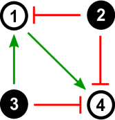
Figure 1: An example network with coherently and incoherently regulated genes. Black and white circles indicate active and inactive nodes, respectively. Node 4 receives coherent input (only repressive) since node 1 is inactive. But node 1 itself is incoherently regulated since it receives conflicting inputs from nodes 2&3.

The degree of coherence for a state ${\bm{\sigma}}$ can then be measured by the fraction of coherent nodes in that state:

$$\alpha_{c}[{\bm{\sigma}}] = \frac{1}{n}\sum_{i}\mbox{int}\left(\left|\sum_{j}c_{ij}\sigma_{j}\right|\bigg{/}\sum_{j}\left|c_{ij}\right|\sigma_{j}\right)\ .$$ (2)

A node with no input (both the numerator and the denominator vanish above) is defined to be perfectly coherent.

We quantify the coherence of the whole network through its steady states (attractors) corresponding to the fixed points or limit cycles of the dynamics, in which a cell spends most of its time. Labelling different steady states with $s$, the global coherence coefficient of the network is expressed as

$$\alpha_{c} = \sum_{s}\frac{w_{s}}{q_{s}}\sum_{i=1}^{q_{s}}\alpha_{c}[{\bm{\sigma}}^{(s)}_{i}]$$ (3)

where $q_{s}$ is the length of the limit cycle $s$ and $w_{s}$ is a weight (such as the relative basin size, i.e., the fraction of initial states that end up in the given attractor) subject to the condition $\sum_{s}w_{s}=1$.

Null-model ensembles:

Bias towards coherent regulation in a GRN can be assessed by comparing $\alpha_{c}$ for the given network with the distribution of the same quantity in a representative ensemble of similar networks. We construct such a reference ensemble separately for each regulatory network detailed in the next section. The ensemble networks were generated by shuffling the edges of the original GRN sufficiently many times such that, the resulting network

• is a connected graph,

• strictly conserves the self edges along with the number of incoming and outgoing activatory/inhibitory interactons separately for each node,

• statistically has no correlation with the original network, except for the local similarities imposed by the two constraints above.

By construction, each gene in these random ensembles is locally subject to the same number of repressory and activatory inputs as in the original network, albeit from possibly different regulatory partners. Under the same rules of dynamics the fixed points and the corresponding $\alpha_{c}$ values are generally different for each random network, since they are determined by the new global structure. For each ensemble, we generated $10^{4}$ non-isomorphic networks and calculated their coherence coefficient both with and without a basin-size dependent weight ($w_{s}$) assigned to each dynamical attractor.

3 Investigated genetic regulatory networks

In this paper, we investigate the degree of coherent regulation in six GRNs associated with different organisms or cell types: cell-cycle networks in Saccharomyces cerevisiae (budding yeast) [47], Scizosaccharomyces pombe (fission yeast) [38] and mammals [39], cell-differentiation networks of Arabidopsis thaliana whorls [50], Th lymphocyte [58] and myeloid progenitors [56]. A graphical description of each GRN is given in Fig 2. These dynamical models were chosen from the literature, subject to the criterion that they reproduce the experimentally observed steady-state expression profile(s) after truncation to Boolean variables. Below, we give a brief description of each GRN.

Figure 2: Gene regulatory networks for (a) Fission yeast cell cycle [38]; (b) Mammalian cell cycle [39]; (c) Budding yeast cell cycle [47]; (d) Arabidopsis thaliana whorl differentiation [50]; (e) Myeloid differentiation [56]; (f) Th-Lymphocyte differentiation [58]. Here green and red edges indicate activation and inhibition respectively which arise through physical or genetic interactions between the nodes representing genes, proteins, protein complexes or transcription factors.

Scizosaccharomyces pombe (fission yeast) cell cycle: The fission yeast cell-cycle network was modeled by Davidich and Bornholdt [38] as a network with 10 nodes (Fig. 2a). The dynamics is governed by threshold functions (see Table 5) which yield 12 fixed points and a fixed cycle. The fixed point with the largest basin matches the biological $G_{1}$ phase.

Mammalian cell cycle: Fauré et al. [39] analysed the regulation dynamics with synchronous, asynchronous, and mixed updating schemes in this GRN model composed of 10 key regulatory elements. Regulation dynamics is given in terms of logical expressions (see Table 4) which are determined according to available experimental evidence for each node. The resulting dynamical attractors are independent of the updating scheme and include a fixed point and a limit cycle, in agreement with the experimental expression data. Note that, the visual depiction of the GRN given in Ref.[39] is inconsistent with the used logic update functions. We here remained faithful to the given logical expressions, after verifying that they reproduce the reported steady states. The structure of the GRN consistent with the interactions in Table 4 is given in Fig. 2b.

Saccharomyces cerevisiae (budding yeast) cell cycle: The model proposed by Li et al [47] is composed of 11 nodes (Fig.2c). This popular model reproduces the G₁ phase as the dominant attractor of a simple Boolean dynamics, as well as the intermediate phases of cell division. Time evolution is governed by threshold functions given in Table 5, which yield 7 fixed point attractors. The attractors other than $G_{1}$ have relatively small basins and, to our knowledge, no clear biological interpretation.

Arabidopsis thaliana whorl differentiation: Mendoza et al. [55] use the network in Fig. 2d in order to model the dynamics of flower morphogenesis. The interactions in the 11-node model network are again inferred from experimental data. Different initial conditions evolved by the proposed rules of dynamics yield 6 point attractors, 4 of which have a clear biological interpretation.

Myeloid differentiation: A Boolean model was set up by Krumsiek et al. [56] in order to understand the mechanisms underlying myeloid differentiation from common myeloid progenitors to megakaryocytes, erythrocytes, granulocytes and monocytes. The 11-node model network (Fig. 2e) is composed of relevant transcription factors which evolve (in time) under separate logical update functions, again inferred from the available experimental evidence. The dynamics gives rise to 5 point attractors, where 4 are in agreement with microarray expression profiles of the mature cell types. It is pointed out that the fifth attractor cannot be realized during physiological hematopoietic differentiation.

Th-Lymphocyte differentiation: Remy et al. [57] proposed this regulatory network model for the differentiation of T-helper lymphocytes (Th0) cells into Th1 and Th2 in the vertebrate immune system. Discrete-time evolution of each node in the model network is governed by node-specific logical rules given in Table 6. The network structure in Fig. 2f is dominated by activatory interactions. The dynamics settles into 3 steady states, in agreeement with the gene expression levels in the Th0, Th1 and Th2 cells.

Organism/Cell type	Func.	Network parameters			# of attr.
		n	k	p	all	bio.
S. pombe	c.c.	10	2.3	0.35	13	1
Mammalian cell	c.c.	10	3.1	0.32	2	2
S. cerevisiae	c.c.	11	2.64	0.51	6	1
A. thaliana whorls	diff.	11	2	0.55	6	4
Myeloid progenitor	diff.	11	2.36	0.42	5	4
Th-lymphocyte	diff.	12	1.67	0.65	6	2

Table 1: Structural/dynamical features associated with the six regulatory networks adopted from the literature. “c.c” and “diff.” refer to regulation of cell cycle and differentiation respectively. Last two columns exclude the trivial point attractor ${\bm{\sigma}}=0$.

It was shown earlier that structural parameters such as the mean number of incoming edges per node ($k$) and the fraction of up-regulating interactions ($p$) in the network are important determinants of global coherence, while the size of the network for fixed $(k,p)$ only weakly influences $\alpha_{c}$ [30]. Observed values of $(n,k,p)$ for each network are listed in Table 1. For the GRNs we consider here, $k$ varies within $[1.67,3.1]$, while $p$ changes in the interval $[0.32,0.65]$ (self-edges are excluded). All models have roughly the same network size ($\sim 11$ nodes).

4 Coherence in biological networks

Table 2 and Fig. 3 summarize the outcome of our coherence analysis on the GRNs depicted in Fig. 2 and listed in section 3. We separately calculated the degree of coherence of each GRN over the full set of fixed points/cycles ($\alpha_{c}$) and over the biologically relevant subset ($\alpha^{bio}_{c}$), both adopted from respective references. We compared them with the mean ($\alpha^{rand}_{c}$) obtained from the associated ensemble of random networks described in Section 2.2.

Organism/Cell type	$\alpha_{c}$ (uniformly weighted)			$\alpha_{c}$ (basin-size weighted)
	$\alpha_{c}$	$\alpha_{c}^{bio}$	$\alpha_{c}^{rand}$	$\alpha_{c}$	$\alpha_{c}^{bio}$	$\alpha_{c}^{rand}$
S. pombe	0.95	1	0.94 $\pm$ 0.04	0.99	1	0.93$\pm$ 0.05
Mammalian cell	0.88	0.88	0.85 $\pm$ 0.07	0.88	0.88	0.86 $\pm$ 0.07
S. cerevisiae	0.97	1	0.80 $\pm$ 0.08	0.99	1	0.75$\pm$ 0.10
A. thaliana whorls	1	1	0.97 $\pm$ 0.04	1	1	0.96 $\pm$ 0.04
Myeloid progenitor	0.89	0.89	0.82 $\pm$ 0.09	0.90	0.88	0.84 $\pm$ 0.09
Th-lymphocyte	0.99	0.96	0.94 $\pm$ 0.05	0.94	0.92	0.94 $\pm$ 0.05

Table 2: Degrees of coherence associated with the regulatory networks shown in Fig. 2. $\alpha_{c}^{all}$, $\alpha_{c}^{bio}$, $\alpha_{c}^{rand}$, denote the coherence value calculated by using Eq.(3) over all attractors of the model dynamics, only the attractors observed in the wild type, and all networks in the corresponding randomized ensemble, respectively.

Our central observation is that, despite the variability in $k$ and $p$, all biological networks are more coherent than random networks constructed with similar structural parameters. Fig. 3 also shows the distribution of $\alpha_{c}$ over the random ensembles for a better judgment of the bias towards coherence. The difference in coherence between the biological network and the random ensemble is visible but within acceptable bounds for most isolated examples. However, the fact that all display a positive deviation from the respective ensemble means suggests an overall preference towards coherence. We quantified the statistically significance of this bias by using Fisher’s method [59] on the present data, which yields a likelihood of $0.044$ and $0.075$ for a chance encounter of a this much or larger deviation in uniformly and basin-weighted cases, respectively. The degree of selection is appreciable, considering that the compared ensemble networks have not only the same number of nodes, the same number of interactions, and the same proportion of repressory/activatory regulation globally, but also the same local pattern of incoming and outgoing edges for each node.

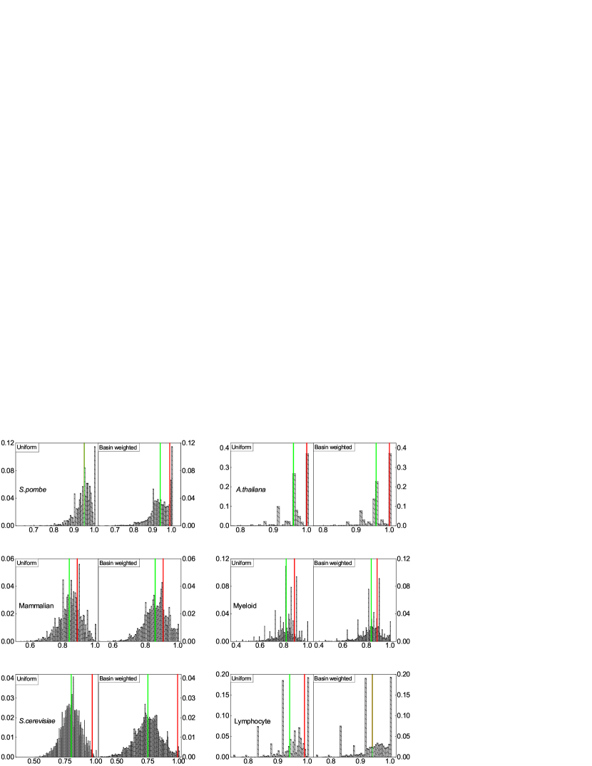
Figure 3: Degree of coherent regulation for biological vs random networks. The histograms of $\alpha_{c}$ for random ensembles of $10^{4}$ networks having similar structure is shown with their mean values (green line). The red line indicates the $\alpha_{c}$ of the biological networks, whose exact values can be seen on Table 2.

5 Coherence vs structural/dynamical network properties

The bias observed in biological regulatory networks above provides motivation to investigate the relationship between coherence and other architectural or dynamical determinants of a network. Identifying such connections could help one recognize coherent systems from certain telltale patterns instead of requiring detailed information about their function, and/or design them by means of simple guiding principles.

Edge number $\&$ type:

We first investigated the dependence of average coherence $\overline{\alpha}_{c}$ on the number of incoming/outgoing edges per node, $k$, and the fraction of activatory interactions, $p$. To this end, we simulated the majority-rule dynamics in Ref. [47] on different $(k,p)$ pairs equally spaced in the rectangle $0.909\leq k\leq 10\ \otimes\ 0\leq p\leq 1$, with $n=11$. The result is shown in Fig. 4. Each data point in Fig. 4 is an average over $10^{3}$ random networks which are generated by random shuffling of edges. No constraint was imposed on the shuffling process, apart from the requirement of connectedness (every node is accessible from every other node in the undirected network).

One observes that, independent of the average connectivity $k$, random networks display minimum coherence when approximately two-thirds ($60-72\%$) of the interactions are activatory. An intuitive understanding of this behavior was proposed in Ref. [30] where a subset of the results in Fig. 4 (for a single $k$ value) was reported.

Coordinates corresponding to the studied biological networks are shown by colored spheres on the same figure. It is interesting that all of them are situated on the low-$p$ slope of the minimum coherence valley.

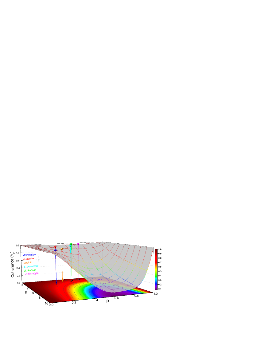
Figure 4: Dependence of coherence value ($\overline{\alpha}_{c}$) on the network parameters ($k,p$) with $n=11$. As $k$ increases from 1 to 10, the $p$ value where $\overline{\alpha}_{c}$ is minumum for the fixed $k$ shifts from 0.72 to 0.6. Coherence values corresponding to the biological networks are shown by spheres.

Number of active genes:

We next asked if the number of active genes $(n_{a})$ at a fixed point/cycle is a determining factor for coherence. After all, coherence reflects the harmony between the regulatory messages originating from these genes. To this end, we considered the attractors found within the ensembles generated by shuffling the edges of each GRN in Fig. 2. We grouped them according to $n_{a}$ and calculated the mean coherence within each group. The results in Fig. 5 show that attractors with higher number of active nodes are generally less coherent. This behavior may be understood by the intuitive fact that it is more difficult to reach consensus in a large group than in a small one. We remind that, this relationship is valid only within the restricted ensembles generated by the shuffling process described in Section 2. One can not speak of a monotonic dependence of coherence on $n_{a}$ if, for example, the difference in $n_{a}$ between two networks is due to different $p$ values. This is evident from the fact that $\bar{n}_{a}(p)$ calculated over the network ensembles used in Fig. 4 trivially increases with $p$ while $\overline{\alpha}_{c}(p)$ is nonmonotonic for any fixed $k$.

Figure 5: Average ratio of active nodes in the point-attractors vs. average coherence in ensembles of model networks. The average is calculated over $10^{4}$ networks chosen randomly from the null-model ensemble described in section 2.2

Basin size:

It is implicit from Table 2 and Fig. 3 that, coherent attractors are not always those with larger basins. We explicitly examined the variation in coherence as a function of the relative basin size of the attractors. The results (Fig. 6), obtained over the networks in the randomized ensembles of each GRN separately, suggest no consistent relation between the basin size and coherence. Likewise, biologically relevant attractors [38, 39, 47, 55, 56, 57] of GRNs in Fig. 2 are not always those with the largest basins. This is hardly surprising, since the initial state prior to differentiation or cell division is never determined randomly.

Figure 6: Average coherence vs. average basin size for the attractors (point or cycles) of $10^{4}$ networks with similar structure. Note that, proposed rules of dynamics in some models appear to prohibit appearance of excessively dominant attractors.

6 Conclusion

We investigated the degree of coherent regulation in several regulatory networks responsible for cell cycle and differentiation in various organisms or cell types, by means of a recently proposed measure of coherence. We found that, even though most networks are moderately more coherent than expected (in reference to architecturally similar network ensembles), cumulatively there is a statistically meaningful bias towards coherence. Our findings lend support to the thesis that pressure for coherent regulation is one of the factors driving the evolution of GRNs. It is not difficult to imagine a Hebbian-like mechanism [60] in the given context, where regulatory interactions incompatible with the required expression profile get eliminated over time. The fact that transcriptional regulatory networks have been observed to have the fastest mutation rate among various biological networks [61] suggests that their evolutionary dynamics may be sufficiently fluid for effective Hebbian selection.

We also showed, on randomly generated model GRNs, that coherence is harder to achieve with increasing number of interactions per node, and with an inhibitory interaction ratio around $1/3$. Furthermore, coherent networks typically involve a smaller number of active genes at their steady states, compared to arbitrary networks with similar edge composition and local connectivity. It could be interesting to focus on networks following the identical expression pattern in time as, say, the yeast cell-cycle (see, e.g., Ref. [62]) and check if those with higher coherence are more similar to their biological counterpart or encompass other desirable properties such as higher robustness or better controllability. Finally, from an architectural perspective, coherence can be viewed as a design choice for any natural or artificial network where inhibitory and activatory interactions coexist. One might then ask how to build a coherent system from scratch, or how to enhance coherence in an existing system with minimal intervention. We hope our findings to trigger further theoretical investigations in these directions.

7 Appendix

Below, we list the rules of regulatory dynamics for each GRN model adopted from the literature.

Network	Gene	Boolean Update Function
Myeloid differentiation	GATA-2	$\textnormal{GATA-2}\wedge\overline{(\textnormal{GATA-1}\wedge\textnormal{FOG-1})}\wedge\overline{\textnormal{PU.1}}$
	GATA-1	$(\textnormal{GATA-1}\vee\textnormal{GATA-2}\vee\textnormal{Fli-1})\wedge\overline{\textnormal{PU.1}}$
	FOG-1	GATA-1
	EKLF	$\textnormal{GATA-1}\wedge\overline{\textnormal{Fli-1}}$
	Fli-1	$\textnormal{GATA-1}\wedge\overline{\textnormal{EKLF}}$
	SCL	$\textnormal{GATA-1}\wedge\overline{\textnormal{PU.1}}$
	C/EBPα	$\textnormal{C/EBP}_{\alpha}\wedge\overline{(\textnormal{GATA-1}\wedge\textnormal{FOG-1}\wedge\textnormal{SCL})}$
	PU.1	$(\textnormal{C/EBP}_{\alpha}\vee\textnormal{PU.1})\wedge\overline{(\textnormal{GATA-1}\vee\textnormal{GATA-2})}$
	cJun	$\textnormal{PU.1}\wedge\overline{\textnormal{Gfi-1}}$
	EgrNab	$(\textnormal{PU.1}\wedge\textnormal{cJun})\wedge\overline{\textnormal{Gfi-1}}$
	Gfi-1	$\textnormal{C/EBP}_{\alpha}\wedge\overline{\textnormal{EgrNab}}$

Table 3: Update functions for myeloid differentiation.

Network	Gene	Boolean Update Functiont
Mammalian cell cycle	CycD	$CycD$
	Rb	$(\overline{CycD}\wedge\overline{CycE}\wedge\overline{CycA}\wedge\overline{CycB})\vee(p27\wedge\overline{CycD}\wedge\overline{CycB})$
	E2F	$(\overline{Rb}\wedge\overline{CycA}\wedge\overline{CycB})\vee(p27\wedge\overline{Rb}\wedge\overline{CycB})$
	CycE	$E2F\wedge\overline{{Rb}}$
	CycA	$(E2F\wedge\overline{Rb}\wedge\overline{Cdc20}\wedge\overline{(Cdh1\wedge Ubc)})\\ \vee(CycA\wedge\overline{Rb}\wedge\overline{Cdc20}\wedge\overline{(Cdh1\wedge Ubc)})$
	p27	$(\overline{CycD}\wedge\overline{CycE}\wedge\overline{CycA}\wedge\overline{CycB})\vee(p27\wedge\overline{(CycE\wedge CycA)}\wedge\overline{CycB}\wedge\overline{CycD})$
	Cdc20α	$CycB$
	Cdh1	$(\overline{CycA}\wedge\overline{CycB})\vee Cdc20\vee(p27\wedge\overline{CycB})$
	UbcH10	$\overline{Cdh1}\vee(Cdh1\wedge Ubc\wedge(Cdc20\vee CycA\vee CycB))$
	CycB	$\overline{Cdc20}\wedge\overline{Cdh1}$

Table 4: Update functions for mammalian cell cycle.

Network	Node $i$	Gene	$\text{Update Function}^{\dagger}$
S. cerevisiae cell cycle	1	Cln3	$S_{i}(t+1)=\left\{\begin{array}[]{ll}1,&\mbox{$I>0$}\\ 0,&\mbox{$I\leq 0$}\\ \end{array}\right.$
	2	Cln1,2
	3	Cdc20
	4	Mcm
	5	Swi5
	6	SBF	$S_{i}(t+1)=\left\{\begin{array}[]{ll}1,&\mbox{$I>0$}\\ 0,&\mbox{$I<0$}\\ S_{i}(t),&\mbox{$I=0$}\\ \end{array}\right.$
	7	MBF
	8	Sic1
	9	Clb5
	10	Cdh1
	11	Clb1
S. pombe cell cycle	1	SK	$S_{i}(t+1)=\left\{\begin{array}[]{ll}1,&\mbox{$I>0$}\\ 0,&\mbox{$I\leq 0$}\\ \end{array}\right.$
	2	SLP
	3	PP
	4	Ste9	$S_{i}(t+1)=\left\{\begin{array}[]{ll}1,&\mbox{$I>\theta_{i}$}\\ 0,&\mbox{$I<\theta_{i}$}\\ S_{i}(t),&\mbox{$I=\theta_{i},$}\\ \end{array}\right.$
	5	Rum1
	6	Cdc2
	7	Cdc2*
	8	Wee1
	9	Cdc25
A. thaliana whorl differentiation	1	EMF1	$S_{i}(t+1)=\left\{\begin{array}[]{ll}1,&\mbox{$I>0$}\\ 0,&\mbox{$I\leq 0$}\\ \end{array}\right.$
	2	TFL1
	3	LFY
	4	AP1
	5	CAL
	6	LUG
	7	UFO
	8	BFU
	9	AG
	10	AP3
	11	PI
	12	SUP
In the update functions $I=\sum_{j=1}^{N}A_{ij}S_{i}(t)$ where $A$ is the weighted adjacency matrix and $\theta$’s indicate the thereshold values for the nodes. For detailed explanations for these values one can refer to [47, 38, 55].

Table 5: Update rules of the regulatory dynamics for the budding yeast (Saccharomyces cerevisiae), the fission yeast (Saccharomyces pombe), and the flower Arabidopsis thaliana.

Network	Gene	Boolean Update Function†
Lymphocyte Differentiation	IFN-$\gamma$	$K_{1}(9),K_{1}(11),K_{1}(9,11)$
	IL-4	$K_{2}(12)$
	IL-12
	IFN-$\gamma$R	$K_{4}(1)$
	IL-4R	$K_{5}(2)$
	IL-12R	$K_{6}(3)$
	STAT1	$K_{7}(4)$
	STAT6	$K_{8}(5)$
	STAT4	$K_{9}(6)$
	SOCS1	$K_{10}(7),K_{10}(11),K_{10}(7,11)$
	T-bet	$K_{11}(7),K_{11}(11),K_{11}(7,11)$
	GATA-3	$K_{12}(8)$
$K_{i}(\{j\})$ is the set of nodes $j$ that when simultaneously active turn the node $i$ on. For details one can refer to [57].

Table 6: Update functions for lymphocyte differentiation.

References

References

- [1] Csikász-Nagy A, Battogtokh D, Chen K C, Novák B and Tyson J J 2006 Biophysical journal 90 4361–4379
- [2] Kashiwagi A, Urabe I, Kaneko K and Yomo T 2006 PloS one 1 e49
- [3] Chaves M, Albert R and Sontag E D 2005 Journal of theoretical biology 235 431–449
- [4] Garg A, Mohanram K, Di Cara A, De Micheli G and Xenarios I 2009 Bioinformatics 25 i101–i109
- [5] Sevim V and Rikvold P A 2008 Journal of theoretical biology 253 323–332
- [6] Kaneko K 2007 PLoS One 2 e434
- [7] Zhou Q, Chipperfield H, Melton D A and Wong W H 2007 Proceedings of the National Academy of Sciences 104 16438–16443
- [8] Kuo-Ching L and Xiaodong W 2008 EURASIP Journal on Bioinformatics and Systems Biology 2008
- [9] Zhou X, Wang X and Dougherty E R 2003 Signal Processing 83 745–761
- [10] Kaneko K 2007 PLoS One 2 e434
- [11] Brooks A N, Turkarslan S, Beer K D, Yin Lo F and Baliga N S 2011 Wiley Interdisciplinary Reviews: Systems Biology and Medicine 3 544–561
- [12] Wang Y and Huang H 2014 Journal of theoretical biology
- [13] Chai L E, Loh S K, Low S T, Mohamad M S, Deris S and Zakaria Z 2014 Computers in biology and medicine 48 55–65
- [14] Davidson E H 2010 Nature 468 911–920
- [15] Peter I S and Davidson E H 2009 FEBS letters 583 3948–3958
- [16] Thomas R and Kaufman M 2001 Chaos: An Interdisciplinary Journal of Nonlinear Science 11 170–179
- [17] Klemm K and Bornholdt S 2005 Proceedings of the National Academy of Sciences of the United States of America 102 18414–18419
- [18] Thieffry D 2007 Briefings in bioinformatics 8 220–225
- [19] Thomas R, Thieffry D and Kaufman M 1995 Bulletin of mathematical biology 57 247–276
- [20] Kaufman M and Thomas R 2003 Comptes rendus biologies 326 205–214
- [21] Burda Z, Krzywicki A, Martin O and Zagorski M 2011 Proceedings of the National Academy of Sciences 108 17263–17268
- [22] Milo R, Shen-Orr S, Itzkovitz S, Kashtan N, Chklovskii D and Alon U 2002 Science Signalling 298 824
- [23] Milo R, Shen-Orr S, Itzkovitz S, Kashtan N, Chklovskii D and Alon U 2002 Science Signalling 298 824
- [24] Cinquin O and Demongeot J 2002 Comptes rendus biologies 325 1085–1095
- [25] Liu Y Y, Slotine J J and Barabási A L 2011 Nature 473 167–173
- [26] Wu Y, Zhang X, Yu J and Ouyang Q 2009 PLoS computational biology 5 e1000442
- [27] Li G W, Burkhardt D, Gross C and Weissman J S 2014 Cell 157 624–635
- [28] Russell J B and Cook G M 1995 Microbiological reviews 59 48–62
- [29] Buttgereit F and Brand M D 1995 Biochem. J 312 163–167
- [30] Aral N and Kabakçıoğlu A 2015 Physical Biology 12 036002
- [31] Rämö P, Kesseli J and Yli-Harja O 2005 Chaos: An Interdisciplinary Journal of Nonlinear Science 15 034101–034101
- [32] Wagner A 2005 Molecular biology and evolution 22 1365–1374
- [33] Willadsen K, Triesch J and Wiles J 2008 Understanding robustness in random boolean networks. ALIFE pp 694–701
- [34] Alon U 2006 An introduction to systems biology: design principles of biological circuits (CRC press)
- [35] Alon U 2007 Nature Reviews Genetics 8 450–461
- [36] Huang S, Eichler G, Bar-Yam Y and Ingber D E 2005 Physical review letters 94 128701
- [37] Luscombe N M, Babu M M, Yu H, Snyder M, Teichmann S A and Gerstein M 2004 Nature 431 308–312
- [38] Davidich M I and Bornholdt S 2008 PLoS One 3 e1672
- [39] Fauré A, Naldi A, Chaouiya C and Thieffry D 2006 Bioinformatics 22 e124–e131
- [40] Fauré A and Thieffry D 2009 Mol. BioSyst. 5 1569–1581
- [41] Lau K Y, Ganguli S and Tang C 2007 Physical Review E 75 051907
- [42] Murata T 1989 Proceedings of the IEEE 77 541–580
- [43] Chaouiya C, Remy E, Ruet P and Thieffry D 2004 Applications and Theory of Petri Nets 2004 137–156
- [44] Karlebach G and Shamir R 2008 Nature Reviews Molecular Cell Biology 9 770–780
- [45] Chen K C, Wang T Y, Tseng H H, Huang C Y F and Kao C Y 2005 Bioinformatics 21 2883–2890
- [46] Chen T, He H L, Church G M et al. 1999 Modeling gene expression with differential equations Pacific symposium on biocomputing vol 4 p 4
- [47] Li F, Long T, Lu Y, Ouyang Q and Tang C 2004 Proceedings of the National Academy of Sciences of the United States of America 101 4781–4786
- [48] Chen K C, Calzone L, Csikasz-Nagy A, Cross F R, Novak B and Tyson J J 2004 Molecular biology of the cell 15 3841–3862
- [49] Davidich M and Bornholdt S 2008 arXiv preprint arXiv:0807.1013
- [50] Mendoza L, Thieffry D and Alvarez-Buylla E R 1999 Bioinformatics 15 593–606
- [51] Albert R and Othmer H G 2003 Journal of theoretical biology 223 1–18
- [52] Gursky V V, Reinitz J and Samsonov A M 2001 Chaos: An Interdisciplinary Journal of Nonlinear Science 11 132–141
- [53] Leloup J C and Goldbeter A 1998 Journal of biological rhythms 13 70–87
- [54] Akman O E, Watterson S, Parton A, Binns N, Millar A J and Ghazal P 2012 Journal of The Royal Society Interface 9 2365–2382
- [55] Mendoza L and Alvarez-Buylla E R 1998 Journal of theoretical biology 193 307–319
- [56] Krumsiek J, Marr C, Schroeder T and Theis F J 2011 PloS one 6 e22649
- [57] Remy E, Ruet P, Mendoza L, Thieffry D and Chaouiya C 2006 Transactions on Computational Systems Biology VII 56–72
- [58] Remy E and Ruet P 2008 Bioinformatics 24 i220–i226
- [59] Fisher R A 1925 Statistical methods for research workers (Genesis Publishing Pvt Ltd)
- [60] Morris R 1999 Brain research bulletin 50 437
- [61] Shou C, Bhardwaj N, Lam H Y, Yan K K, Kim P M, Snyder M and Gerstein M B 2011 PLoS Comput Biol 7 e1001050–e1001050
- [62] Lau K Y, Ganguli S and Tang C 2007 Physical Review E 75 051907