Astronomy Letters, 2015, Vol. 41, No. 9, pp. 473–488.

Determination of the Galactic Rotation Curve from OB Stars

V.V. Bobylev and A. T. Bajkova

Pulkovo Astronomical Observatory, St. Petersburg, Russia

Abstract—We consider three samples of O- and B-type stars from the solar neighborhood 0.6–4 kpc for which we have taken the distances, line-of-sight velocities, and proper motions from published sources. The first sample contains 120 massive spectroscopic binaries. O stars with spectroscopic distances from Patriarchi et al. constitute the second sample. The third sample consists of 168 OB3 stars whose distances have been determined from interstellar calcium lines. The angular velocity of Galactic rotation at the solar distance $\Omega_{0},$ its two derivatives $\Omega^{\prime}_{0}$ and $\Omega^{\prime\prime}_{0},$ and the peculiar velocity components of the Sun $(U,V,W)_{\odot}$ are shown to be well determined from all three samples of stars. They are determined with the smallest errors from the sample of spectroscopic binary stars and the sample of stars with the calcium distance scale. The fine structure of the velocity field associated with the influence of the Galactic spiral density wave clearly manifests itself in the radial velocities of spectroscopic binary stars and in the sample of stars with the calcium distance scale.

INTRODUCTION

Young massive stars of spectral types O and B are visible from great distances from the Sun. Therefore, they are an important tool for studying the structure and kinematics of the Galaxy (Moffat et al. 1998; Zabolotskikh et al. 2002; Avedisova 2005; Popova and Loktin 2005). Since OB stars do not recede far from their birthplaces in their lifetime, they trace well the spiral structure of the Galaxy (Efremov 2011; Coleiro and Chaty 2013; Vallée 2014; Hou and Han 2014).

So far the distances to active star-forming regions, where OB stars are concentrated, have been determined by the kinematic method (Anderson et al. 2012), which has a low accuracy (Moisés 2011). The spectroscopic and photometric distance estimation methods can be used only for a relatively small solar neighborhood with a radius of 4–5 kpc. However, several factors presently reduce the accuracy of these methods. First, there are virtually no direct measurements of the parallaxes for supergiants in the Hipparcos catalogue (1997) with an accuracy of at least 10%. Such measurements are needed to establish a reliable calibration. Second, the uncertainty in establishing the spectral type and luminosity class is great for high-luminosity stars. According to Wegner (2007), the first two factors cause, for example, the absolute magnitude dispersion for the sequences of Ia or Iab supergiants on the Hertzsprung–Russell diagram to be about 1.5–2.0 magnitudes (this dispersion is only about 0.3 magnitude for main-sequence stars). Third, for the application of photometric methods (for example, based on Strömgren photometry), there are simply no data for distance determinations.

The appearance of infrared observations, in particular, the 2MASS catalogue (Skrutskie et al. 2006), has contributed to an increase in the accuracy of these methods when the interstellar extinction is taken into account. Using the photometric characteristics from this catalogue, Patriarchi et al. (2003) determined the spectroscopic distances for 184 O stars. One of our goals is to study the Galactic kinematics using data on these stars.

Spectroscopic binaries are of interest in their own right. They usually have a long history of observations. The systemic line-of-sight velocities, spectral classification, and photometry are well known for many of them. Having analyzed the detached spectroscopic binaries with known spectroscopic orbits selected on condition that the masses and radii of both components were determined with errors of no more than 3%, Torres et al. (2010) showed their spectroscopic distances to agree with the trigonometric ones within error limits of no more than 10%. In Eker et al. (2014), the number of such binaries was increased by 67%; it is 257. However, the fraction of young massive binaries among them is small (about 20 binaries).

Previously (Bobylev and Bajkova 2013a), we presented a kinematic database containing information about 220 massive young stars. The stars are no farther than 3–4 kpc from the Sun; about 100 of them are spectroscopic binary and multiple systems whose components are massive OB stars, while the rest are B stars from the Hipparcos catalogue with spectral types no later than B2.5 and errors in the trigonometric parallaxes no more than 10%. All stars have estimates of their proper motions, line-of-sight velocities, and distances, which allows their space velocities to be analyzed. A significant fraction of the stars from this sample (162 stars) belongs to the Gould Belt (with heliocentric distances $r<0.6$ kpc). Previously (Bobylev and Bajkova 2013a, 2014b), we analyzed the kinematics and spatial distribution of these nearby stars. In contrast, the number of more distant stars (58 stars at $r>0.6$ kpc) should be increased for a reliable determination of the parameters describing the Galactic kinematics.

At present, there are estimates of the distances to OB stars made by the spectroscopic method from the broadening of interstellar Ca II, Na I, or K I absorption lines (Megier et al. 2005, 2009), with this scale having been reconciled with the trigonometric parallaxes (Megier et al. 2005). Quite recently, new measurements of stars performed by this method have been published (Galazutdinov et al. 2015).

The goal of this paper is to expand the kinematic database on massive young star systems, to compare the various distance scales, and to determine the parameters of the Galactic rotation and spiral density wave based on the data obtained.

METHOD

From observations we know three projections of the stellar velocity: the line-of-sight velocity $V_{r}$ as well as the two velocities $V_{l}=4.74r\mu_{l}\cos b$ and $V_{b}=4.74r\mu_{b}$ directed along the Galactic longitude $l$ and latitude $b$ and expressed in km s^-1. Here, the coefficient 4.74 is the ratio of the number of kilometers in an astronomical unit to the number of seconds in a tropical year, and $r$ is the heliocentric distance of the star $r$ in kpc. The proper motion components $\mu_{l}\cos b$ and $\mu_{b}$ are expressed in milliarcseconds per year (mas yr^-1). The velocities $U,V,$ and $W$ directed along the rectangular Galactic coordinate axes are calculated via the components $V_{r},V_{l},$ and $V_{b}:$

$$\begin{array}[]{lll}U=V_{r}\cos l\cos b-V_{l}\sin l-V_{b}\cos l\sin b,\\ V=V_{r}\sin l\cos b+V_{l}\cos l-V_{b}\sin l\sin b,\\ W=V_{r}\sin b+V_{b}\cos b,\end{array}$$ (1)

where $U$ is directed from the Sun to the Galactic center, $V$ is in the direction of Galactic rotation, and $W$ is directed toward the north Galactic pole. We can find two velocities, $V_{R}$ directed radially away from the Galactic center and $V_{circ}$ orthogonal to it and pointing in the direction of Galactic rotation, based on the following relations:

$$\begin{array}[]{lll}V_{circ}=U\sin\theta+(V_{0}+V)\cos\theta,\\ V_{R}=-U\cos\theta+(V_{0}+V)\sin\theta,\end{array}$$ (2)

where the position angle $\theta$ is calculated as $\tan\theta=y/(R_{0}-x),$ while $x$ and $y$ are the rectangular Galactic coordinates of the star. $\Omega_{0}$ is the angular velocity of Galactic rotation at the solar distance $R_{0},$ the parameters $\Omega^{\prime}_{0}$ and $\Omega^{\prime\prime}$ are the corresponding derivatives of the angular velocity, and $V_{0}=|R_{0}\Omega_{0}|.$

The velocities $V_{R}$ and $W$ are virtually independent of the pattern of the Galactic rotation curve. However, to analyze any periodicities in the tangential velocities, it is necessary to determine a smoothed Galactic rotation curve and to form the residual velocities $\Delta V_{circ}.$ As experience shows, to construct a smooth Galactic rotation curve in a wide range of distances $R,$ it is usually sufficient to know two derivatives of the angular velocity, $\Omega^{\prime}_{0}$ and $\Omega^{\prime\prime}_{0}$. Note that all three velocities $V_{R},$ $\Delta V_{circ},$ and $W$ must be freed from the peculiar solar velocity $U_{\odot},V_{\odot},W_{\odot}$.

To determine the parameters of the Galactic rotation curve, we use the equations derived from Bottlinger’s formulas in which the angular velocity $\Omega$ was expanded in a series to terms of the second order of smallness in $r/R_{0}:$

$$\begin{array}[]{lll}V_{r}=-U_{\odot}\cos b\cos l-V_{\odot}\cos b\sin l\\ -W_{\odot}\sin b+R_{0}(R-R_{0})\sin l\cos b\Omega^{\prime}_{0}+0.5R_{0}(R-R_{0})^{2}\sin l\cos b\Omega^{\prime\prime}_{0},\end{array}$$ (3)

$$\begin{array}[]{lll}V_{l}=U_{\odot}\sin l-V_{\odot}\cos l-r\Omega_{0}\cos b\\ +(R-R_{0})(R_{0}\cos l-r\cos b)\Omega^{\prime}_{0}+0.5(R-R_{0})^{2}(R_{0}\cos l-r\cos b)\Omega^{\prime\prime}_{0},\end{array}$$ (4)

$$\begin{array}[]{lll}V_{b}=U_{\odot}\cos l\sin b+V_{\odot}\sin l\sin b\\ -W_{\odot}\cos b-R_{0}(R-R_{0})\sin l\sin b\Omega^{\prime}_{0}-0.5R_{0}(R-R_{0})^{2}\sin l\sin b\Omega^{\prime\prime}_{0},\end{array}$$ (5)

where $R$ is the distance from the star to the Galactic rotation axis,

$$R^{2}=r^{2}\cos^{2}b-2R_{0}r\cos b\cos l+R^{2}_{0}.$$ (6)

The influence of the spiral density wave in the radial, $V_{R},$ and residual tangential, $\Delta V_{circ},$ velocities is periodic with an amplitude of $\sim$10 km s${}^{-1}.$ According to the linear theory of density waves (Lin and Shu 1964), it is described by the following relations:

$$\begin{array}[]{lll}V_{R}=-f_{R}\cos\chi,\\ \Delta V_{circ}=f_{\theta}\sin\chi,\end{array}$$ (7)

where

$$\chi=m[\cot(i)\ln(R/R_{0})-\theta]+\chi_{\odot}$$ (8)

is the phase of the spiral density wave ($m$ is the number of spiral arms, $i$ is the pitch angle of the spiral pattern, $\chi_{\odot}$ is the radial phase of the Sun in the spiral density wave); $f_{R}$ and $f_{\theta}$ are the radial and tangential velocity perturbation amplitudes, which are assumed to be positive.

In the next step, we apply a spectral analysis to study the periodicities in the velocities $V_{R}$ and $\Delta V_{circ}$. The wavelength $\lambda$ (the distance between adjacent spiral arm segments measured along the radial direction) is calculated from the relation

$$\frac{2\pi R_{0}}{\lambda}=m\cot(i).$$ (9)

Let there be a series of measured velocities $V_{R_{n}}$ (these can be both radial, $V_{R}$ and residual tangential, $\Delta V_{\theta},$ velocities), $n=1,\dots,N$, where $N$ is the number of objects. The objective of our spectral analysis is to extract a periodicity from the data series in accordance with the adopted model describing a spiral density wave with parameters $f_{R},\lambda(i)$ and $\chi_{\odot}$.

Having taken into account the logarithmic character of the spiral density wave and the position angles of the objects $\theta_{n},$ our spectral (periodogram) analysis of the series of velocity perturbations is reduced to calculating the square of the amplitude (power spectrum) of the standard Fourier transform (Bajkova and Bobylev 2012):

$$\bar{V}_{\lambda_{k}}=\frac{1}{N}\sum_{n=1}^{N}V^{{}^{\prime}}_{n}(R^{{}^{\prime}}_{n})\exp\Bigl{(}-j\frac{2\pi R^{{}^{\prime}}_{n}}{\lambda_{k}}\Bigr{)},$$ (10)

where $\bar{V}_{\lambda_{k}}$ is the $k$th harmonic of the Fourier transform with wavelength $\lambda_{k}=D/k,D$ is the period of the series being analyzed,

$$\begin{array}[]{lll}R^{{}^{\prime}}_{n}=R_{\circ}\ln(R_{n}/R_{\circ}),\\ V^{{}^{\prime}}_{n}(R^{{}^{\prime}}_{n})=V_{n}(R^{{}^{\prime}}_{n})\times\exp(jm\theta_{n}).\end{array}$$ (11)

The algorithm of searching for periodicities modified to properly determine not only the wavelength but also the amplitude of the perturbations is described in detail in Bajkova and Bobylev (2012).

Таблица 1: Bibliographic information about the stars

Star	$V_{\gamma}$, $\leavevmode\nobreak\ \mu,\leavevmode\nobreak\$ $dist$	Star	$V_{\gamma}$, $\leavevmode\nobreak\ \mu,\leavevmode\nobreak\$ $dist$
MWC 1	Sb9, L07, G12	Herschel 36	Ar10, UC4, Ar10
V745 Cas	Ch14a, L07, Ch14a	V411 Ser	Sb9, L07, G12
BM Cas	Sb9, L07, Pop77	mu. Sgr	Sb9, L07, BB15
HD 12323	Sb9, UC4, Gal15	16 Sgr	Ma14, L07, G12
V622 Per	Mal07, UC4, Cap02	MY Ser	Ib13, L07, Ib13
V615 Cas	MJ14, MJ14, MJ14	QR Ser	S09, L07, S09
V482 Cas	Sb9, Tyc2, Mc03	RY Sct	Sb9, L07, Sm02
MY Cam	Lr14, Tyc2, Lr14	MCW 715	Sb9, L07, Hut71
KS Per	Sb9, L07, BB15	V337 Aql	Tu14, Tu14, Tu14
HD 31617	Sb9, L07, Gui12	MWC 314	Lo13, Tyc2, Car10
HD 31894	Sb9, L07, Gui12	V1765 Cyg	Sb9, L07, G12
eps Aur	Sb9, L07, Gui12	V380 Cyg	Sb9, L07, Tk14
ADS 4072AB	Sb9, L07, Pat03	HD 124314	SIMB, L07, G12
3 Pup	Sb9, L07, RR94	V2107 Cyg	B14, L07, B14
HD 72754	Sb9, L07, L07	ALS 10885	G06, L07, Pat03
ALS 1803	Sb9, L07, Pat03	V470 Cyg	Sb9, L07, Com12
ALS 1834	Sb9, Tyc2, Pat03	WR 140	Sb9, Dz09, Do05
V560 Car	Sb9, Tyc2, R01	V404 Cyg	MJ14, MJ14, MJ14
V346 Cen	Sb9, UC4, Ka10	Schulte 73	Ki09, UC4, Ki09
KX Vel	Ma14, L07, Ma14	V382 Cyg	Sb9, L07, YY12
HD 97166	Ma14, UC4, Ma14	V2186 Cyg	Ki12, UC4, Ki12
HD 115455	Ma14, UC4, Ma14	MT91 771	Ki12, UC4, Ki07
HD 123590	Ma14, L07, Av84	VV Cep	Sb9, L07, L07
HD 150136	S13, UC4, S13	V2174 Cyg	Sb9, L07, Bol78
HD 152234	Sb9, L07, G12	4U 2206+54	StZ14, Tyc2, SIMB
HD 152246	Na14, L07, Na14	V446 Cep	Ch14b, L07, Ch14b
Braes 144	SIMB, Tyc2, G12	MWC 656	Cas14, L07, Cas14
V1297 Sco	SIMB, Tyc2, G12	GT Cep	Ch15, L07, Ch15
Pismis 24-1	MW07, Tyc2, MW07	V373 Cas	Sb9, L07, Hl87
HD 163892	Ma14, L07, CaII	ALS 12775	Sb9, L07, BB15
HR 6716	Sb9, L07, St99	VZ Cen	Wil13, L07, BB15

1. The sources of line-of-sight velocities: Sb9 (Pourbaix et al. 2004); Ch14a, Ch14b, Ch15 (Çhakirli et al. 2014a, 2014b, 2015); Ar10 (Arias et al. 2010); Ma14 (Mayer et al. 2014); G06 (Gontcharov 2006); Mal07 (Malchenko et al. 2007); Ib13 (Ibanoglu et al. 2013); MJ14 (Miller-Jones 2014); S09, S13 (Sana et al. 2009, 2013); Lr14 (Lorenzo et al. 2014); Tu14 (Tüysüz et al. 2014); StZ14 (Stoyanov et al. 2014); Ki07, Ki09, Ki12 (Kiminki et al. 2007, 2009, 2012); Lo13 (Lobel et al. 2013); B14 (Bakiş et al. 2014); Na14 (Nasseri et al. 2014); Cas14 (Casares et al. 2014); MW07 (Maiz-Apellániz et al. 2007); Wil13 (Williams et al. 2013); SIMB (SIMBAD database).

2. The sources of proper motions: L07 (van Leeuwen 2007); UC4 (UCAC4, Zacharias et al. 2012); Tyc2 (Tycho-2, Hog et al. 2000); Dz09 (Dzib and Rodriguez 2009).

3. The sources of distances: G12 (Gudennavar et al. 2012); CaII (Megier et al. 2009); Pat03 (Patriarchi et al. 2003); Pop77 (Popper 1977); Gal15 (Galazutdinov et al. 2015); Cap02 (Capilla and Fabregat 2002); Mc03 (McSwain 2003); Sm02 (Smith et al. 2002); Av84 (Avedisova and Kondratenko 1984); Bol78 (Bolton and Rogers 1978); Hut71 (Hutchings and Redman 1971); Gui12 (Guinan 2012); Car10 (Carmona et al. 2010); R01 (Rauw et al. 2001); RR94 (Rovero and Ringuelet 1994); Com12 (Comerón and Pasquali 2012); Do05 (Dougherty et al. 2005); Hl87 (Hill and Fisher 1987); St99 (Stickland and Lloyd 1999); Tk14 (Tkachenko et al. 2014); Ka10 (Kaltcheva and Scorcio 2010); BB15 (our estimates); YY12 (Yaşarsoy and Yakut 2012).

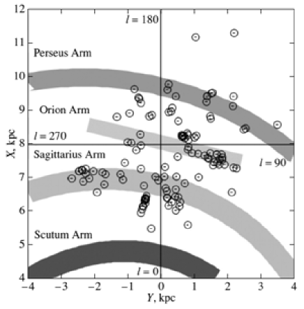
Рис. 1: Distribution of 120 spectroscopic binary stars in projection onto the Galactic $XY$ plane; the Sun is at the intersection of the dashed lines; the fragments of the four-armed spiral pattern are indicated; the position of the local spur, the Orion arm, is marked.

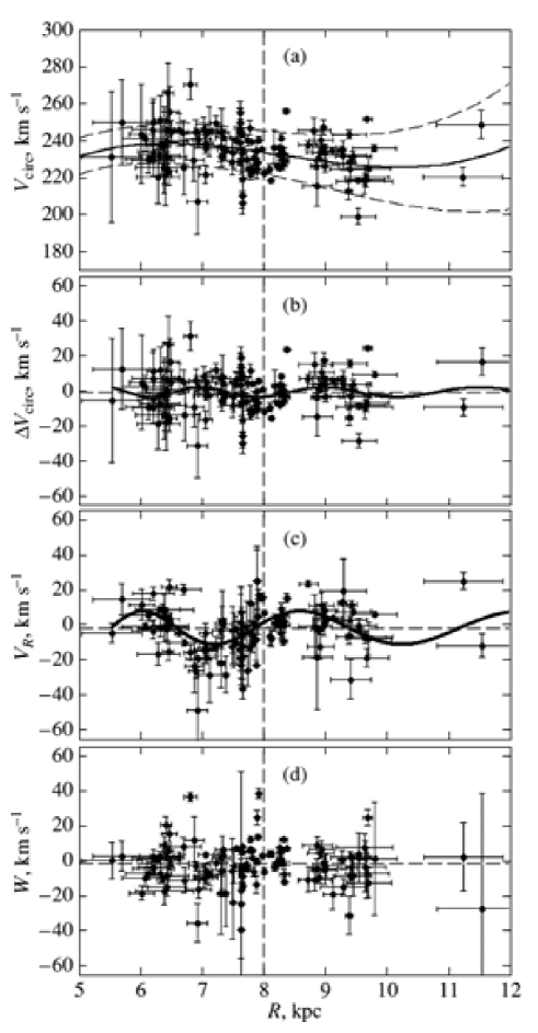
Рис. 2: (a) Galactic rotation curve constructed from the sample of 120 spectroscopic binary stars with parameters (13) with an indication of the boundaries of the 1$\sigma$ confidence intervals; residual rotation velocities $\Delta V_{circ}$ (b), radial velocities $V_{R}$ (c), and vertical velocities $W$ (d) of stars versus $R;$ the vertical dashed line marks the Sun’s position.

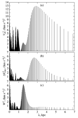
Рис. 3: Power spectra of the radial, $V_{R}$, residual tangential, $\Delta V_{circ},$ and vertical, $W,$ velocities for the sample of spectroscopic binary stars.

DATA

The Sample of Spectroscopic Binary OB Stars

To select young massive distant spectroscopic binaries, we used the SB9 database (Pourbaix et al. 2004), which contains references to the spectroscopic orbit determinations up until 2014. We considered binaries with spectral types of the primary component no later than B2.5 and various supergiants with luminosity classes Ia and Iab. Thus, we are interested in stars with masses of more than 10 solar masses.

For a preliminary distance estimate, we consulted various sources, for example, the compiled database by Gudennavar et al. (2012) and the FUSE (Far Ultraviolet Spectroscopic Explorer) survey (Bowen et al. 2008). Finally, the publications of various authors that determine orbits are an important source of information.

We did not consider stars nearer than 0.6 kpc, where the Gould Belt dominates, and stars farther than 4 kpc, where the proper motion errors are great. We added 62 more binaries that possess no properties of ‘‘runaway’’ stars (their residual velocities do not exceed 40–50 km s^-1) to the 58 already described in Bobylev and Bajkova (2013a). Bibliographic information about these binaries is given in the table. There are cases where there is no orbit in the SB9 catalogue, while it is specified in the SIMBAD database that the star is a spectroscopic binary, for example, HD 124314.

For a number of stars, we calculated the distances by ourselves. The abbreviation BB15 is used for them in the table. Here, we calculated the distances using the photometric magnitudes from the SIMBAD database based on the well-known relation

$$\log r=1+0.2((V-M_{v})-A_{v}),$$ (12)

where $A_{v}=3.2E(B-V),$ $E(B-V)=(B-V)-(B-V)_{0}.$ We took the absolute magnitudes of the stars $M_{v}$ from Wegner (2007), where they were determined from Hipparcos stars for all spectral types and luminosity classes, and the unreddened colors of the stars $(B-V)_{0}$ from Straizys (1977).

The final sample of spectroscopic binaries contains 120 stars. Their distribution in the Galactic $XY$ plane is presented in Fig. 1. The figure shows a fragment of the global four-armed (one of the four arms, the Outer one, is not visible here) spiral pattern with a pitch angle of 13^∘. The pattern was constructed in our previous paper (Bobylev and Bajkova 2014a), where we analyzed the distribution of Galactic masers with measured trigonometric parallaxes. The line segment between the Perseus and Carina–Sagittarius Arms indicates the Local Arm model (Bobylev and Bajkova 2014b). As can be seen from the figure, the distribution of stars agrees well with the plotted spiral pattern. Unfortunately, there are few stars in the third quadrant in the Perseus Arm. In this paper, we take the Galactocentric distance of the Sun to be $R_{0}=8.0\pm 0.4$ kpc.

O Stars from the List by Patriarchi et al. (2003)

Patriarchi et al. (2003) determined the spectroscopic distances for 184 O-type stars; photometric data from the 2MASS catalogue were used to take into account the interstellar extinction. This sample consists mostly of single stars, although there are also spectroscopic binaries in it.

The proper motions from the Hipparcos catalogue revised by van Leeuwen (2007) or from Tycho-2 (Hog et al. 2000) and line-of-sight velocities (according to the SIMBAD database) are known for 156 stars from this list. However, the information is complete only for 101 of them, i.e., their distances, proper motions, and line-of-sight velocities are known simultaneously. The distribution of 156 O stars in projection onto the Galactic $XY$ plane is given in Fig. 4. Just as in Fig. 1, the spiral arms are plotted. The agreement of the stars from this sample with the plotted spiral pattern is noticeably poorer than that for the stars in Fig. 1. Here, we see a larger dispersion of the coordinates in the Carina–Sagittarius Arm toward the Galactic center $(l=0^{\circ}),$ in the Perseus Arm toward the Galactic anticenter $(l=180^{\circ}),$ and, finally, the Orion Arm segment is noticeably stretched in a direction near $l=75^{\circ}$.

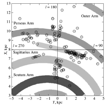
Рис. 4: Distribution of 156 O stars from the list by Patriarchi et al. (2003) in projection onto the Galactic $XY$ plane; the Sun is at the intersection of the dashed lines; the fragments of the four-armed spiral pattern are indicated; the position of the local spur, the Orion Arm, is marked.

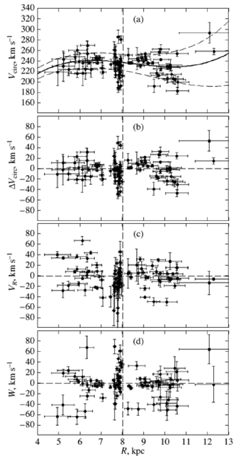
Рис. 5: Galactic rotation curve constructed from the sample of 101 O stars from the list by Patriarchi et al. (2003) with parameters (14) with an indication of the boundaries of the 1$\sigma$ confidence intervals (a); residual rotation velocities $\Delta V_{circ}$ (b), radial velocities $V_{R}$ (c), and vertical velocities $W$ (d) of stars versus $R;$ the vertical dashed line marks the Sun’s position.

The Distances Determined from Interstellar Ca II Lines

The distances to OB stars determined by the spectroscopic method from the broadening of interstellar Ca II, Na I, or K I absorption lines are of indubitable interest. The method of determining such distances is well known. However, the ‘‘calcium’’ distance scale has been tied to the Hipparcos trigonometric parallaxes only recently (Megier et al. 2005). The assumption about a uniform distribution of ionized atoms in the Galactic plane underlies the method. In some places (for example, toward the cluster Trumpler 16), the nonuniformities in the distribution of matter can be significant, which can increase the dispersion of the distance estimates by this method. On average, according to the estimates by Megier et al. (2009), the accuracy of determining the individual distances to OB stars is $\approx$15%.

The first catalogue (Megier et al. 2009) contains 290 OB stars, while Galazutdinov et al. (2015) determined the distances to 61 more OB stars by this method, with the line-if-sight velocities having been measured for all of them. Since the two samples have overlaps, the total number of stars in this distance scale is about 340.

Previously (Bobylev and Bajkova 2011, 2013b), we studied a sample of 258 Hipparcos O–B3 stars with distances from Megier et al. (2009). About 20% of the sample are either known runaway stars or candidates for runaway stars, because they have large ($>40$ km s^-1) residual space velocities. As a result, the range of distances 0.8–3.5 kpc was represented by 102 stars. A slight, no more than 20%, reduction of the distance scale was shown to be necessary by analyzing several kinematic parameters obtained from this sample (Bobylev and Bajkova 2011). In this paper, we use the entire sample, and not only the Hipparcos stars.

Figure 6 gives the distribution of 168 OB stars with distances in the calcium distance scale in the Galactic $XY$ plane for two distance scale factors. In the first case, this factor is equal to one; in the second case, the distances to the stars were multiplied by 0.8. Note that the new measurements by Galazutdinov et al. (2015) were performed exclusively in two narrow sectors: in directions $l\approx 135^{\circ}$ and $l\approx 190^{\circ}$ with heliocentric distances of about 2.3 kpc. Two structures elongated along the line of sight are clearly seen in Fig. 6 in these directions.

RESULTS

Spectroscopic Binary

Using 120 spectroscopic binaries, we found the following kinematic parameters from a least-squares solution of the system of conditional equations (3)–(5):

$$\begin{array}[]{lll}(U_{\odot},V_{\odot},W_{\odot})=(2.8,9.2,9.3)\pm(1.0,1.2,1.0)\leavevmode\nobreak\ \hbox{km s${}^{-1}$},\\ \Omega_{0}=\leavevmode\nobreak\ 29.3\pm 0.8\leavevmode\nobreak\ \hbox{km s${}^{-1}$ kpc${}^{-1}$},\\ \Omega^{{}^{\prime}}_{0}=-4.28\pm 0.15\leavevmode\nobreak\ \hbox{km s${}^{-1}$ kpc${}^{-2}$},\\ \Omega^{{}^{\prime\prime}}_{0}=0.957\pm 0.128\leavevmode\nobreak\ \hbox{km s${}^{-1}$ kpc${}^{-3}$}.\end{array}$$ (13)

In this solution, the error per unit weight is $\sigma_{0}=10.5$ km s^-1. For the adopted $R_{0}=8.0\pm 0.4$ kpc, the linear Galactic rotation velocity $V_{0}=|R_{0}\Omega_{0}|$ is $234\pm 14$ km s^-1, while the Oort constants are $A=-17.1\pm 0.6$ km s^-1 kpc^-1 and $B=12.2\pm 1.0$ km s^-1 kpc^-1. The Galactic rotation curve constructed with parameters (13) and the residual tangential, $\Delta V_{circ},$ radial, $V_{R},$ and vertical, $W,$ velocities of stars as a function of the distance R are given in Fig. 2.

Why are the vertical velocities $W$ given in Fig. 2? The point is that periodic vertical velocity oscillations have been detected quite recently in Galactic masers with measured trigonometric parallaxes (Bobylev and Bajkova 2015). Such oscillations with an amplitude of about 4–6 km s^-1 can be associated with the influence of the Galactic spiral density wave. Therefore, confirming this phenomenon in the velocities of other samples of stars with different distance scales is of great interest.

Based on a spectral analysis, we determined the parameters of the spiral density wave using the sample of spectroscopic binary stars. The results are reflected in Fig. 3, where the power spectra of the radial, $V_{R},$ residual tangential, $\Delta V_{circ}$, and vertical, $W,$ velocities are given. Note that there is a high significance of the signal, $p=0.999,$ only in the power spectrum of the radial velocities. For the tangential velocities, the significance of the signal at a wavelength $\lambda\approx 2.6$ kpc is $p=0.898.$ As can be seen on the middle panel in Fig. 3, there are spurious signals in the range of short wavelengths whose amplitudes exceed the amplitude of the signal of interest to us. There are also spurious signals in the power spectrum of the vertical velocities $W,$ while the signal at a wavelength of about 1.5 kpc agrees poorly with the two preceding graphs.

As a result, for the model of a four-armed spiral pattern $(m=4),$ we found the amplitudes of the velocity perturbations $f_{R}=9.5\pm 1.5$ km s^-1 and $f_{\theta}=3.2\pm 1.4$ km s^-1 in the radial and tangential directions, respectively, the wavelength $\lambda_{R}=2.8\pm 0.5$ kpc (then, $i_{R}=-13^{\circ}\pm 4^{\circ}$) and $\lambda_{\theta}=2.6\pm 0.4$ kpc (then, $i_{\theta}=-12^{\circ}\pm 3^{\circ}$) at the Sun’s phase in the spiral density wave $(\chi_{\odot})_{R}=-95^{\circ}\pm 15^{\circ}$, and $(\chi_{\odot})_{\theta}=-93^{\circ}\pm 12^{\circ},$ respectively. The corresponding waves are given on panels (b) and (c) in Fig. 2. Their logarithmic character is clearly seen.

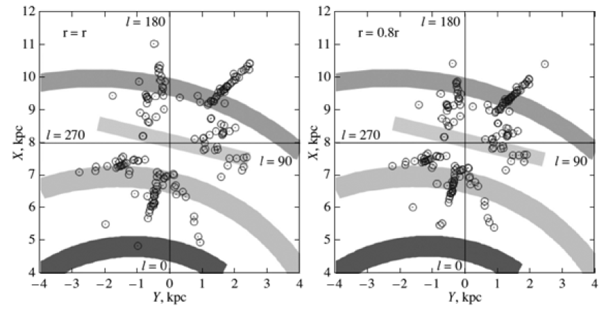
Рис. 6: Distribution of 168 OB stars with distances in the ‘‘calcium’’ distance scale in projection onto the Galactic $XY$ plane (a); the distances to these stars were multiplied by factor of 0.8 (b); the fragments of the four-armed spiral pattern and the position of the Orion Arm are indicated.

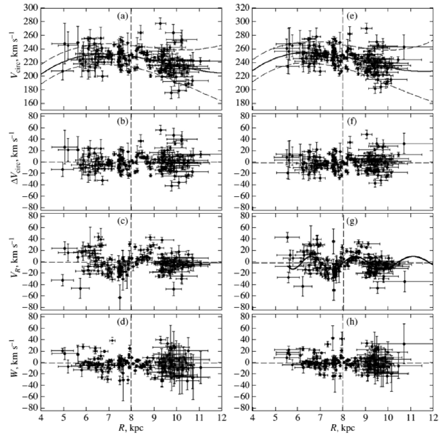
Рис. 7: Galactic rotation curve constructed from 168 OB stars with distances in the original ‘‘calcium’’ scale (a); residual rotation velocities $\Delta V_{circ}$ (b), radial velocities $V_{R}$ (c), and vertical velocities $W$ (d) of stars versus $R;$ the same dependences are given on panels (e)–(g) for the stars whose distances were reduced by 20%.

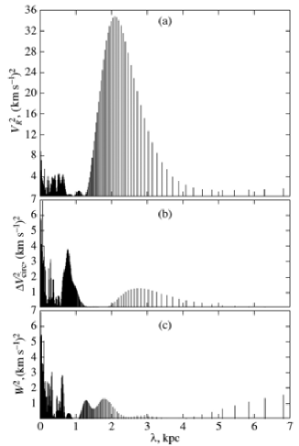
Рис. 8: Power spectra of the radial, $V_{R},$ residual tangential, $\Delta V_{circ},$ and vertical, $W,$ velocities for the sample of OB3 stars with the calcium distance scale.

Stars from Patriarchi et al. (2003)

Using 156 O stars from the list by Patriarchi et al. (2003), we found the following parameters:

$$\begin{array}[]{lll}(U_{\odot},V_{\odot},W_{\odot})=(5.8,16.9,8.6)\pm(2.1,2.6,1.8)\leavevmode\nobreak\ \hbox{km s${}^{-1}$},\\ \Omega_{0}=\leavevmode\nobreak\ 29.6\pm 1.2\leavevmode\nobreak\ \hbox{km s${}^{-1}$ kpc${}^{-1}$},\\ \Omega^{{}^{\prime}}_{0}=-4.27\pm 0.27\leavevmode\nobreak\ \hbox{km s${}^{-1}$ kpc${}^{-2}$},\\ \Omega^{{}^{\prime\prime}}_{0}=0.910\pm 0.143\leavevmode\nobreak\ \hbox{km s${}^{-1}$ kpc${}^{-3}$}.\end{array}$$ (14)

In this solution, the error per unit weight is $\sigma_{0}=21.9$ km s^-1, and the linear Galactic rotation velocity is $V_{0}=237\pm 15$ km s^-1 for $R_{0}=8.0\pm 0.4$ kpc.

There are quite a few stars without line-of-sight velocities in this list. Equations (3)–(5) can be solved with limited information, which was done when obtaining solution (14). However, complete information is needed to calculate the velocities $\Delta V_{circ},V_{R},$ and $W,$ i.e., only 101 stars can be used.

The Galactic rotation curve constructed with parameters (14) and the residual tangential, $\Delta V_{circ},$ radial, $V_{R},$ and vertical, $W,$ velocities of stars as a function of the distances $R$ are given in Fig. 5. It can be seen from this figure that a smooth Galactic rotation curve is determined quite well. Since the velocities $\Delta V_{circ},$ $V_{R},$ and $W$ are fairly irregular in pattern, we did not perform a spectral analysis of these velocities.

The error per unit weight $\sigma_{0}$ characterizes the dispersion of the residuals in the least-squares solution of the system of equations (3)–(5). Its value is usually close to the value of the residual velocity dispersions for the sample stars averaged over all directions (the ‘‘cosmic’’ velocity dispersion). The value of $\sigma_{0}=21.9$ km s^-1 found in solution (14) is twice $\sigma_{0}\approx 10$ km s^-1 expected for OB stars. This may imply that the errors in the distances and, consequently, the tangential velocities of these stars are too great. Panel (d) in Fig. 5, on which large vertical velocities $W$ are seen for a considerable number of stars, attracts our attention.

We produced a new sample of stars with space velocities for two constraints: $|W|<40$ km s^-1 and $|z|<100$ pc. Applying these constraints allows the number of possible runaway stars to be reduced significantly. 61 stars satisfy these criteria. Using them, we found the following parameters:

$$\begin{array}[]{lll}(U_{\odot},V_{\odot},W_{\odot})=(10.1,14.6,5.7)\pm(2.1,2.3,1.9)\leavevmode\nobreak\ \hbox{km s${}^{-1}$},\\ \Omega_{0}=\leavevmode\nobreak\ 31.7\pm 1.5\leavevmode\nobreak\ \hbox{km s${}^{-1}$ kpc${}^{-1}$},\\ \Omega^{{}^{\prime}}_{0}=-4.53\pm 0.29\leavevmode\nobreak\ \hbox{km s${}^{-1}$ kpc${}^{-2}$},\\ \Omega^{{}^{\prime\prime}}_{0}=1.124\pm 0.247\leavevmode\nobreak\ \hbox{km s${}^{-1}$ kpc${}^{-3}$},\end{array}$$ (15)

where the error per unit weight is $\sigma_{0}=13.7$ km s^-1, which is considerably smaller than that in solution (14).

The ‘‘Calcium’’ Distance Scale

Based on 168 stars, we obtained the following solution for the adopted $R_{0}=8.0\pm 0.4$ kpc:

$$\begin{array}[]{lll}(U_{\odot},V_{\odot},W_{\odot})=\\ (10.2,9.3,9.5)\pm(1.1,1.6,1.1)\leavevmode\nobreak\ \hbox{km s${}^{-1}$},\\ \Omega_{0}=\leavevmode\nobreak\ 28.7\pm 0.9\leavevmode\nobreak\ \hbox{km s${}^{-1}$ kpc${}^{-1}$},\\ \Omega^{{}^{\prime}}_{0}=-4.21\pm 0.16\leavevmode\nobreak\ \hbox{km s${}^{-1}$ kpc${}^{-2}$},\\ \Omega^{{}^{\prime\prime}}_{0}=0.652\pm 0.149\leavevmode\nobreak\ \hbox{km s${}^{-1}$ kpc${}^{-3}$},\end{array}$$ (16)

$\sigma_{0}=13.6$ km s^-1 and $V_{0}=230\pm 15$ km s^-1. Based on the same stars, we also obtained the solution for the distance scale factor 0.8:

$$\begin{array}[]{lll}(U_{\odot},V_{\odot},W_{\odot})=\\ (10.4,9.7,7.0)\pm(1.0,1.4,0.9)\leavevmode\nobreak\ \hbox{km s${}^{-1}$},\\ \Omega_{0}=\leavevmode\nobreak\ 31.3\pm 0.9\leavevmode\nobreak\ \hbox{km s${}^{-1}$ kpc${}^{-1}$},\\ \Omega^{{}^{\prime}}_{0}=-4.78\pm 0.16\leavevmode\nobreak\ \hbox{km s${}^{-1}$ kpc${}^{-2}$},\\ \Omega^{{}^{\prime\prime}}_{0}=0.864\pm 0.176\leavevmode\nobreak\ \hbox{km s${}^{-1}$ kpc${}^{-3}$},\end{array}$$ (17)

$\sigma_{0}=11.6$ km s^-1 и $V_{0}=250\pm 15$ km s^-1. Figure 7 gives the Galactic rotation curve and the velocities $\Delta V_{circ},$ $V_{R},$ and $W$ as a function of R constructed from OB stars with distances in the original calcium scale and the scale reduced by 20%.

Based on a spectral analysis, we determined the parameters of the spiral density wave from the sample of spectroscopic binary stars with the reduced distance scale. The results are reflected in Fig. 8, where the power spectra of the radial, $V_{R},$ residual tangential, $\Delta V_{circ},$ and vertical, $W,$ velocities are given. Note that there is a high significance of the signal, $p=0.999,$ only in the power spectrum of the radial velocities. It can be clearly seen on panels (b) and (c) that there is no statistically significant signal with a wavelength of about 2.5 kpc typical of the spiral density wave for the tangential and vertical velocities.

As a result, from our analysis of the radial velocities we found the velocity perturbation amplitude $f_{R}=11.8\pm 1.3$ km s^-1 and the wavelength $\lambda=2.1\pm 0.4$ kpc ($i=-9.5^{\circ}\pm 1.7^{\circ}$) at the Sun’s phase in the spiral density wave $\chi_{\odot}=-86^{\circ}\pm 7^{\circ}$. This wave is given on panel (g) in Fig. 7.

DISCUSSION

First of all, it should be noted that the peculiar solar velocity components, the angular velocity of Galactic rotation, and its two derivatives, are determined quite well from all three samples of stars. They are determined with the smallest errors from the sample of spectroscopic binary stars and the sample of stars with the calcium distance scale.

For two samples, we also determined such kinematic parameters previously, but only using a smaller number of stars. The results of solution (13) should be compared with the results of our analysis for 58 distant spectroscopic binary stars outside the circle with a radius of 0.6 kpc (Bobylev and Bajkova 2013a): $(U_{\odot},V_{\odot})=(2.2,8.4)\pm(0.9,1.1)$ km s^-1 and $\Omega_{0}=31.9\pm 1.1$ km s^-1 kpc^-1, $\Omega^{{}^{\prime}}_{0}=-4.30\pm 0.16$ km s^-1 kpc^-2, $\Omega^{{}^{\prime\prime}}_{0}=1.05\pm 0.35$ km s^-1 kpc^-3, where the error per unit weight is $\sigma_{0}=9.9$ km s^-1 and $V_{0}=255\pm 16$ km s^-1.

Based on a sample of 102 OB3 stars with the calcium distance scale (and the scale factor 0.8), previously (Bobylev and Bajkova 2011) we found the following parameters: $(U_{\odot},V_{\odot},W_{\odot})=(8.9,10.3,6.8)\pm(0.6,1.0,0.4)$ km s^-1, $\Omega_{0}=31.5\pm 0.9$ km s^-1 kpc^-1, $\Omega^{{}^{\prime}}_{0}=-4.49\pm 0.12$ km s^-1 kpc^-2, $\Omega^{{}^{\prime\prime}}_{0}=1.05\pm 0.38$ km s^-1 kpc^-3, the error per unit weight was $\sigma_{0}=9.6$ km s^-1, and the circular rotation velocity was $V_{0}=252\pm 14$ km s^-1 ($R_{0}=8$ kpc). We can see good agreement with solution (17). The only difference is that the error in the second derivative of the angular velocity $\Omega^{{}^{\prime\prime}}_{0}$ decreased considerably with increasing number of stars.

The distances for the O stars from the list by Patriarchi et al. (2003) were determined not quite reliably. Note that these authors took the absolute magnitudes of the stars $M_{v}$ from the rather old paper by Panagia (1973) and their spectral types from the catalogue by Garmany et al. (1982). The correct spectral classification is of great importance in determining the spectroscopic distances of stars. A telling example is the star HD 160641, for which the spectral type O9.5I is specified in the catalogue by Patriarchi et al. (2003), and the distance $r=9$ kpc was calculated. According to the estimates by a number of authors, this is a helium star, a sdOc9.5II-III:He40 dwarf (Drilling et al. 2013) with a mass of $\sim$1$M_{\odot}$. In this case, the distance to the star is $r=3.3\pm 0.8$ kpc (Lynas-Gray et al. 1987).

Why does the sample of spectroscopic binaries look better? After all, the distances to the stars were determined either by the photometric method or by the spectroscopic one. In our view, the fact that each star is ‘‘piece goods’’ when the spectroscopic orbits are determined plays a role here. In this case, the authors have a detailed idea of the binary characteristics, in particular, of the spectra of the binary components; therefore, the inaccuracies in the spectral classification are minimal.

At present, there is a sample of approximately 100 maser sources whose trigonometric parallaxes have been measured by the VLBI method with a very high accuracy, with a mean error of $\pm 20$ $\mu$as and, for some of them, with a record error of $\pm 5\leavevmode\nobreak\ \mu$as. From an analysis of these masers, Reid et al. (2014) found the velocity of the Sun $V_{0}=240\pm 8$ km s^-1 ($R_{0}=8.34\pm 0.16$ kpc). Previously, based on a smaller number of masers, Honma et al. (2012) obtained an estimate of $V_{0}=238\pm 14$ km s^-1 ($R_{0}=8.05\pm 0.45$ kpc). It can be seen that the values of this velocity found in this paper are in good agreement with the best present day estimates.

Based on a sample of masers, previously (Bobylev and Bajkova 2015) we found the following parameters of the spiral density wave for $m=4:$ $f_{\theta}=6.0\pm 2.6$ km s^-1, $f_{R}=7.2\pm 2.2$ km s^-1, $\lambda_{\theta}=3.2\pm 0.5$ kpc, $\lambda_{R}=3.0\pm 0.6$ kpc, $(\chi_{\odot})_{\theta}=-79^{\circ}\pm 14^{\circ}$ and $(\chi_{\odot})_{R}=-199^{\circ}\pm 16^{\circ}$. The values found in this paper from the sample of spectroscopic binary stars are fairly close to them. The values found from the radial velocities of stars with the calcium distance scale are characterized by a larger amplitude and a smaller $(\chi_{\odot})_{R}.$ However, this just confirms the results of our previous analysis (Bobylev and Bajkova 2011).

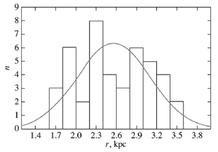
Рис. 9: Distribution of 43 stars with the calcium distance scale on the line of sight in the direction $l=135^{\circ};$ a Gaussian with a mean of 2.56 pc and a dispersion of 0.54 pc was fitted.

Given the rather significant relative errors in the distances for many of the stars being used, the question about the systematic bias in the mean distances of the remaining stars arises. Obviously, there are relatively more objects with overestimated distances among the rejected stars farther than 4 kpc and, on the contrary, with underestimated distances among the stars nearer than 600 pc. Such a bias in the distances is related to the Lutz–Kelker effect (Lutz and Kelker 1973; Stepanishchev and Bobylev 2013). For the classical case where a uniform distribution of stars is adopted, we can use a formula of the form (Lutz and Kelker 1973)

$$F(z)={1\over z^{4}}\exp{\biggl{[}-{(z-1)^{2}\over 2\sigma_{p}^{2}}\biggr{]}},$$ (18)

where $z=\pi/\pi_{0}$ is the ratio of the true parallax $\pi$ to the observed parallax $\pi_{0},$ $\sigma_{p}=\sigma_{0}/\pi_{0}$ is the relative error of the observed parallax, and $F(z)$ is the probability density.

We took the mean error in the distances for the spectroscopic binaries and the stars with the calcium distance scale to be 15%. The mean correction for the Lutz–Kelker effect for these stars is then 100 pc (the measured distances should be increased). For the stars from the list by Patriarchi et al. (2003), we took the error in the distance for each star to be 30%. As a result of our simulations, we found that the total bias for these stars due to the Lutz–Kelker effect could be 240 pc.

The chains of stars elongated along the line of sight, which can be seen in Fig. 4 and particularly clearly in Fig. 6, deserve special attention. The most plausible explanation is that there are large relative errors in the distances to the objects that actually belong to a single compact grouping (a cluster, an association, or a stellar complex). Based on such objects, we obtained an independent estimate of the relative error in the distance using stars with the calcium distance scale as an example. The result is reflected in Fig. 9, where the distribution of 43 OB stars with the calcium distance scale lying on the line of sight in the direction $l=135^{\circ}$ is given. Based on the parameters of the fitted Gaussian (a mean of 2.56 pc and a dispersion of 0.54 pc), we find the relative error in the distance to be 21%. The mean value calculated from the individual distance errors for these stars is 0.42; the relative error in the distance is then 16%.

CONCLUSIONS

We considered O- and B-type stars located in a wide solar neighborhood, with distances from 0.6 to 4 kpc. We produced three samples of stars for which the distances, line-of-sight velocities, and proper motions collected from published data were available. The first sample includes 120 massive (with masses $>10M_{\odot}$) spectroscopic binaries. O stars for which Patriarchi et al. (2003) estimated the spectroscopic distances using infrared photometric data from the 2MASS catalogue constitute the second sample. Single stars constitute the overwhelming majority in this sample. The third sample consists of 168 OB3 stars whose distances were determined from interstellar calcium lines. As in the previous case, mostly single stars enter into this sample.

Such kinematic parameters as the angular velocity of Galactic rotation at the solar distance $\Omega^{\prime}_{0},$ its two derivatives $\Omega^{\prime}_{0},$ and $\Omega^{\prime\prime}_{0}$ and the peculiar solar velocity components $(U,V,W)_{\odot}$ were shown to be well determined from all three samples of stars. They are determined with the smallest errors from the sample of spectroscopic binaries and the sample of stars with the calcium distance scale.

The fine structure of the velocity field associated with the influence of the Galactic spiral density wave clearly manifests itself in the radial velocities of the spectroscopic binaries and in the sample of stars with the calcium distance scale. No small-amplitude periodic oscillations in the vertical velocities with a wavelength of about 2.5 kpc manifest themselves in any of the stellar samples considered in this paper. The available accuracies of the distances are probably insufficient for a reliable detection of such oscillations.

The linear rotation velocity of the Galaxy $V_{0}$ was found from the sample of spectroscopic binary stars to be $234\pm 14$ km s^-1 (for the adopted $R_{0}=8.0\pm 0.4$ kpc). Based on a spectral analysis of the radial and tangential velocities for these stars, we determined the parameters of the spiral density wave. For the model of a four-armed spiral pattern $(m=4),$ we found the following: the perturbation velocity amplitudes $f_{R}=9.5\pm 1.5$ km s^-1 and $f_{\theta}=3.2\pm 1.4$ km s^-1 in the radial and tangential directions, respectively; the wavelength $\lambda_{R}=2.8\pm 0.5$ kpc (then, $i_{R}=-13^{\circ}\pm 4^{\circ}$) at the Sun’s phase in the spiral density wave $(\chi_{\odot})_{R}=-95^{\circ}\pm 15^{\circ}$ and $\lambda_{\theta}=2.6\pm 0.4$ kpc (then, $i_{\theta}=-12^{\circ}\pm 3^{\circ}$) at the Sun’s phase $(\chi_{\odot})_{\theta}=-93^{\circ}\pm 12^{\circ}.$

The velocity $V_{0}=250\pm 15$ km s^-1 (for $R_{0}=8.0\pm 0.4$ kpc and a distance scale factor of 0.8) was found from the sample of OB3 stars with the calcium distance scale. The parameters of the spiral density wave were determined only by analyzing the radial velocities. The perturbation velocity amplitude is $f_{R}=11.8\pm 1.3$ km s^-1 and the wavelength is $\lambda_{R}=2.1\pm 0.3$ kpc ($m=4,$ $i_{R}=-9.5^{\circ}\pm 1.7^{\circ}$) at the Sun’s phase in the spiral density wave $(\chi_{\odot})_{R}=-86^{\circ}\pm 7^{\circ}$.

ACKNOWLEDGMENTS

We are grateful to the referees for their useful remarks that contributed to an improvement of the paper. This work was supported by the ‘‘Transient and Explosive Processes in Astrophysics’’ Program P–41 of the Presidium of the Russian Academy of Sciences. The SIMBAD electronic astronomical database was widely used in our work.

REFERENCES

1. L.D. Anderson, T.M. Bania, D.S. Balser, and R.T. Rood, Astrophys. J. 754, 62 (2012).

2. J.I. Arias, R.H. Barbá, R.C. Gamen, N.I. Morrell, J. Maiz-Apellániz, E.J. Alfaro, A. Sota, N.R. Walborn, and C. M. Bidin, Astrophys. J. Lett. 710, L30 (2010).

3. V.S. Avedisova and G.I. Kondratenko, Nauchn. Inform. Astron. Sov. AN SSSR 56, 59 (1984).

4. V.S. Avedisova, Astron. Rep. 49, 435 (2005).

5. A.T. Bajkova and V.V. Bobylev, Astron. Lett. 38, 549 (2012).

6. V. Bakiş, H. Hensberge, S. Bilir, H. Bakiş, F. Yilmaz, E. Kiran, O. Demircan, M. Zejda, and Z. Mikulašek, Astron. J. 147, 149 (2014).

7. V.V. Bobylev and A.T. Bajkova, Astron. Lett. 37, 526 (2011).

8. V.V. Bobylev and A.T. Bajkova, Astron. Lett. 39, 532 (2013a).

9. V.V. Bobylev and A.T. Bajkova, Astron. Nachr. 334, 768 (2013b).

10. V.V. Bobylev and A.T. Bajkova, Mon. Not. R. Astron. Soc. 437, 1549 (2014a).

11. V.V. Bobylev and A.T. Bajkova, Astron. Lett. 40, 783 (2014).

12. V.V. Bobylev and A.T. Bajkova, Mon. Not. R. Astron. Soc. 447, L50 (2015).

13. C. T. Bolton and G. L. Rogers, Astrophys. J. 222, 234 (1978).

14. D. V. Bowen, E.B. Jenkins, T.M. Tripp, K.R. Sembach, B. D. Savage, H.W. Moos, W.R. Oegerle, S.D. Friedman, et al., Astrophys. J. Suppl. Ser. 176, 59 (2008).

15. G. Capilla and J. Fabregat, Astron. Astrophys. 394, 479 (2002).

16. A. Carmona, M.E. van den Ancker, M. Audard, Th. Henning, J. Setiawan, and J. Rodmann, Astron. Astrophys. 517, 67 (2010).

17. J. Casares, I. Negueruela, M. Ribó, I. Ribas, J.M. Paredes, A. Herrero, and S. Simón-Diaz, Nature 505, 378 (2014).

18. Ö. Çhakirli, C. Ibanoglu, and E. Sipahi, Mon. Not. R. Astron. Soc. 442, 1560 (2014a).

19. Ö. Çhakirli, C. Ibanoglu, E. Sipahi, A. Frasca, and G. Catanzaro, arXiv:1406.0499 (2014b).

20. Ö. Çhakirli, New Astron. 35, 71 (2015).

21. A. Coleiro and S. Chaty, Astrophys. J. 764, 185 (2013).

22. F. Comerón and A. Pasquali, Astron. Astrophys. 543, 101 (2012).

23. S.M. Dougherty, A.J. Beasley, M.J. Claussen, B.A. Zauderer, and N.J. Bolingbroke, Astrophys. J. 623, 447 (2005).

24. J.S. Drilling, C.S. Jeffery, U. Heber, S. Moehler, and R. Napiwotzki, Astron. Astrophys. 551, 31 (2013).

25. S. Dzib and L.F. Rodriguez, Rev. Mex. Astron. Astrofis. 45, 3 (2009).

26. Yu.N. Efremov, Astron.Rep. 55, 108 (2011).

27. Z. Eker, S. Bilir, F. Soydugan, E.Y. Gökçe, M. Soydugan, M. Tüysüz, T. Şenyüz, and O. Demircan, Publ. Astron. Soc. Austral. 31, 23 (2014).

28. G.A. Galazutdinov, A. Strobel, F.A. Musaev, A. Bondar, and J. Krelowski, Publ. Astron. Soc. Pacif. 127, 126 (2015).

29. C.D. Garmany, P.S. Conti, and C. Chiosi, Astrophys. J. 263, 777 (1982).

30. G.A. Gontcharov, Astron. Lett. 32, 795 (2006).

31. S.B. Gudennavar, S.G. Bubbly, K. Preethi, and J. Murthy, Astrophys. J. Suppl. Ser. 199, 8 (2012).

32. E.F. Guinan, P. Mayer, P. Harmanec, H. Božić, M. Brož, J. Nemravová, S. Engle, et al., Astron. Astrophys. 546, 123 (2012).

33. G.Hill and W.A. Fisher,Astron. Astrophys. 171, 123 (1987).

34. E. Hog, C. Fabricius, V.V. Makarov, S. Urban, T. Corbin, G. Wycoff, U. Bastian, P. Schwekendiek, and A. Wicenec, Astron. Astrophys. 355, L 27 (2000).

35. M. Honma, T. Nagayama, K. Ando, T. Bushimata, Y.K. Choi, T. Handa, et al., Publ. Astron. Soc. Jpn. 64, 136 (2012).

36. L.G. Hou and J.L. Han, Astron. Astrophys. 569, 21 (2014).

37. J.B. Hutchings and R.O. Redman, Mon. Not. R. Astron. Soc. 163, 219 (1971).

38. C. Ibanoglu, Ó. Çakirli, and E. Sipahi, Mon. Not. R. Astron. Soc. 436, 750 (2013).

39. N. Kaltcheva and M. Scorcio, Astron. Astrophys. 514, 59 (2010).

40. D.C. Kiminki, H.A. Kobulnicky, K. Kinemuchi, J.S. Irwin, et al., Astrophys. J. 664, 1102 (2007).

41. D.C. Kiminki, H.A. Kobulnicky, I. Gilbert, S. Bird, and G. Chunev, Astron. J. 137, 4608 (2009).

42. D.C. Kiminki, H.A. Kobulnicky, I. Ewing, M.M.B. Kiminki, M. Lundquist, M. Alexander, C. Vargas-Alvarez, H. Choi, and C.B. Henderson, Astrophys. J. 747, 41 (2012).

43. F. van Leeuwen, Astron. Astrophys. 474, 653 (2007).

44. C.C. Lin and F.H. Shu, Astrophys. J. 140, 646 (1964).

45. A. Lobel, J. Groh, C. Martayan, Y. Frémat, K.T. Dozinel, G. Raskin, et al., Astron. Astrophys. 559, 16 (2013).

46. J. Lorenzo, I.Negueruela, A.K.F. val Baker, M. Garcia, S. Simón-Diaz, P. Pastor, and M. Méndez Majuelos, Astron. Astrophys. 572, 110 (2014).

47. T.E. Lutz and D.H. Kelker,Publ. Astron. Soc. Pacif. 85, 573 (1973).

48. A.E. Lynas-Gray, D. Kilkenny, I. Skillen, and C. F. Jeffery, Mon. Not. R. Astron. Soc. 227, 1073 (1987).

49. J. Maiz-Apellániz, N.R. Walborn, N.I. Morrell, V.S. Niemela, and E.P. Nelan, Astrophys. J. 660, 1480 (2007).

50. S.L. Malchenko, A.E. Tarasov, and K. Yakut, Odessa Astron. Publ. 20, 120 (2007).

51. P. Mayer, H. Drechsel, and A. Irrgang, Astron. Astrophys. 565, 86 (2014).

52. M.V. McSwain, Astrophys. J. 595, 1124 (2003).

53. A. Megier, A. Strobel, A. Bondar, F.A. Musaev, I. Han, J. Krelowski, and G.A. Galazutdinov, Astrophys. J. 634, 451 (2005).

54. A. Megier, A. Strobel, G.A. Galazutdinov, and J. Krelowski, Astron. Astrophys. 507, 833 (2009).

55. J.C.A. Miller-Jones, Publ. Astron. Soc. Austral. 31, 16 (2014).

56. A.E.J. Moffat, S.V. Marchenko, W. Seggewiss, K.A. van der Hucht, H. Schrijver, B. Stenholm, et al., Astron. Astrophys. 331, 949 (1998).

57. A.P. Moisés, A. Damineli, E. Figueredo, R.D. Blum, P. Conti, and C. L. Barbosa, Mon. Not. R. Astron. Soc. 411, 705 (2011).

58. A. Nasseri, R. Chini, P. Harmanec, P. Mayer, J.A. Nemravová, T. Dembsky, H. Lehmann, H. Sana, and J.-B. le Bouquin, Astron. Astrophys. 568, 94 (2014).

59. N. Panagia, Astron. J. 78, 929 (1973).

60. P. Patriarchi, L. Morbidelli, and M. Perinotto, Astron. Astrophys. 410, 905 (2003).

61. M.E. Popova and A.V. Loktin, Astron. Lett. 31, 663 (2005).

62. D.M. Popper, Publ. Astron. Soc. Pacif. 89, 315 (1977).

63. D. Pourbaix, A.A. Tokovinin, A.H. Batten, F.C. Fekel, W.I. Hartkopf, H. Levato, N.I. Morell, G. Torres, and S. Udry, Astron. Astrophys. 424, 727 (2004).

64. G. Rauw, H. Sana, I.I. Antokhin, N.I. Morrell, V.S. Niemela, J.F.A. Colombo, E. Gosset, and J.-M. Vreux, Mon. Not. R. Astron. Soc. 326, 1149 (2001).

65. M.J. Reid, K.M. Menten, A. Brunthaler, X.W. Zheng, T.M. Dame, Y. Xu, et al., Astrophys. J. 783, 130 (2014).

66. A.C. Rovero and A.E. Ringuelet, Mon. Not. R. Astron. Soc. 266, 203 (1994).

67. H. Sana, E. Gosset, and C.J. Evans, Mon. Not. R. Astron. Soc. 400, 1479 (2009).

68. H. Sana, J.-B. Le Bouquin, L. Mahy, O. Absil, M. De Becker, and E. Gosset, Astron. Astrophys. 553, 131 (2013).

69. M.F. Skrutskie, R.M. Cutri, R. Stiening, et al., Astron. J. 131, 1163 (2006).

70. N. Smith, R.D. Gehrz, O. Stahl, B. Balick, and A. Kaufer, Astrophys. J. 578, 464 (2002).

71. A.S. Stepanishchev and V.V. Bobylev, Astron. Lett. 39, 185 (2013).

72. D.J. Stickland and C. Lloyd, Observatory 119, 16 (1999).

73. K.A. Stoyanov, R.K. Zamanov, G.Y. Latev, A.Y. Abedin, and N.A. Tomov, Astron. Nachr. 335, 1060 (2014).

74. V. Straizys, Multicolor Stellar Photometry (Pachart, Tucson, 1992).

75. A. Tkachenko, P. Degroote, C. Aerts, K. Pavlovski, J. Southworth, P.I. Pápics, et al., Mon. Not. R. Astron. Soc. 438, 3093 (2014).

76. G. Torres, J. Andersen, and A. Giménez, Astron. Astrophys. Rev. 18, 67 (2010).

77. M. Tüysüz, F. Soydugan, S. Bilir, E. Soydugan, T. Senyüz, and T. Yontan, New Astron. 28, 44 (2014).

78. J.P. Vallée, Mon. Not. R. Astron. Soc. 442, 2993 (2014).

79. W. Wegner, Mon. Not. R. Astron. Soc. 374, 1549 (2007).

80. S.J. Williams, D.R. Gies, T.C. Hillwig, M.V. McSwain, and W. Huang, in Proceedings of the Conference on Massive Stars: From $\alpha$ to $\Omega$, June 10–14, 2013, Rhodes, Greece (2013).

81. B. Yaşarsoy and K. Yakut, Astrophys. J. 145, 9 (2013).

82. M.V. Zabolotskikh, A.S. Rastorguev, and A.K. Dambis, Astron. Lett. 28, 454 (2002).

83. N. Zacharias, C.T. Finch, T.M. Girard, A. Henden, J.L. Bartlett, D.G. Monet, and M.I. Zacharias, Catalogue No. I/322, Strasbourg DataBase (2012).

84. The Hipparcos and Tycho Catalogues, ESA SP–1200 (1997).