Randomized Approximations of the Image Set of Nonlinear Mappings with Applications to Filtering

Abstract

The aim of this paper is twofold: In the first part, we leverage recent results on scenario design to develop randomized algorithms for approximating the image set of a nonlinear mapping, that is, a (possibly noisy) mapping of a set via a nonlinear function. We introduce minimum-volume approximations which have the characteristic of guaranteeing a low probability of violation, i.e., we admit for a probability that some points in the image set are not contained in the approximating set, but this probability is kept below a pre-specified threshold $\varepsilon$. In the second part of the paper, this idea is then exploited to develop a new family of randomized prediction-corrector filters. These filters represent a natural extension and rapprochement of Gaussian and set-valued filters, and bear similarities with modern tools such as particle filters.
Keywords: Randomized algorithms, filtering, nonlinear systems, semialgebraic sets.
This research was partly funded by CNR-CNRS bilateral project No. 134562.

1 Introduction

In recent years, randomized algorithms have gained increasing popularity in the field of control of uncertain systems; e.g., see Calafiore et al. (2011); Tempo et al. (2013), due to their ability of dealing with large and complex uncertainty structures, thus extending the applicability of the robust control methods. This is obtained by shifting from the robustness paradigm, where one looks for guaranteed performance which should hold for every possible instance of the uncertainty, to an approach where probabilistic guarantees are accepted, i.e., performance is guaranteed only within a given level of probability $\varepsilon>0$. The main technical tool that permits to obtain computationally tractable solutions are randomized algorithms, which could be seen as extensions of the classical Monte Carlo method, and are based on the extraction of random samples of the uncertainty.

In this paper, we exploit these ideas for finding reliable approximations of the image of a set through a nonlinear mapping, which we refer to as the image set. This set is in general nonconvex (possibly not connected), so that classical approximations may be rather difficult to compute and in general may turn out to be very conservative.

The first part of the paper adapts and significantly extends recent results presented by some of the authors in Dabbene et al. (2010), where a new definition of “goodness” of approximation was provided in probabilistic terms. Namely, an approximating set $\mathcal{A}$ of a set $\mathcal{X}$ is deemed to be “good” if it contains “most” of the points in $\mathcal{X}$ with high probability. Contrary to classical approximating sets, which are generally either outer or inner, the ensuing approximating set “optimally describes” the set without neither containing nor being contained in it. This new concept allows to obtain generally tighter approximations, providing a probabilistic characterization of the set, which is particularly appealing in many contexts (even if it may not be desired in others, such e.g. as safety analysis). We recall that outer bounding sets, that is, approximations which are guaranteed to contain the set $\mathcal{X}$, have been very popular in the set-membership approach, and have been used in designing set-theoretic state estimators for uncertain discrete-time nonlinear dynamic systems; e.g., see El Ghaoui and Calafiore (2001); Alamo et al. (2008). Inner ellipsoidal approximations have been introduced for instance in the context of nonlinear programming problems (Nesterov and Nemirovski, 1994) and tolerance design (Wojciechowski and Vlach, 1993).

In Sections II and III, the results of Dabbene et al. (2010) are particularized to the specific problem at hand, and are also generalized by considering a new family of approximating sets which are based on the construction of minimum volume polynomial superlevel sets, recently introduced in Dabbene and Henrion (2013). With these approximating sets, the original convexity requirement can be relaxed, since they can be nonconvex/nonconnected, thus allowing for better descriptions.

The second part of the paper extends these ideas to the design of probabilistic filters for nonlinear discrete time dynamical systems subject to random uncertainty. In particular, the image set approximation is used to design a probabilistically optimal predictor filter. The rationale behind this approach is to “describe” the state position at step $k$ by a set where the state lies with high probability. The prediction step is then combined with a correction step where the propagated set is trimmed based on the available measurements at time $k$ and on the measurement noise assumptions. A detailed discussion on the proposed randomized prediction correction filter is given in Section IV, where a discussion on the related literature is also reported. Numerical examples conclude the paper.

Notation: For a symmetric matrix $P$, $P\succ 0$ means that $P$ is positive definite. We denote by $\mathcal{B}_{p}$ the unit ball in the $\ell_{p}$ norm: $\mathcal{B}_{p}\doteq\left\{z\in{{\mathbb{R}}^{n}}\,:\,\|z\|_{p}\leq 1\right\}.$ The volume or, more precisely, the Lebesgue measure of a compact set $\mathcal{X}$ is denoted by $\mathrm{vol}\,\mathcal{X}\doteq\int_{\mathcal{X}}\mathrm{d}x.$ The uniform measure over $\mathcal{X}$ is denoted by ${{\lambda}}_{\mathcal{X}}$, i.e. ${{\lambda}}_{\mathcal{X}}$ is such that, for any set $\mathcal{Y}\subseteq\mathcal{X}$, ${{\lambda}}_{\mathcal{X}}(\mathcal{Y})=\mathrm{vol}\,\mathcal{Y}/\mathrm{vol}\,\mathcal{X}$. The set of all polynomials of order less than or equal to $\sigma$ is denoted by $\mathbb{P}_{\sigma}$. The monomial basis for this set is represented by the (column) vector $\pi_{\sigma}(x)$ and any polynomial $q\in\mathbb{P}_{\sigma}$ can be expressed in the form $q(x)=\pi_{\sigma}^{\top}(x)q=\pi^{\top}_{\lceil\sigma/2\rceil}(x)Q\pi_{\lceil\sigma/2\rceil}(x)$ where $q$ is a vector and $Q$ is a symmetric matrix of appropriate dimensions, referred to as the Gram matrix.

2 Minimum volume approximations

Consider the following nonlinear mapping:

$$x_{+}=f\bigl{(}x,w\bigr{)}$$ (1)

which represents the one-step evolution of a discrete-time dynamical system, with $x,x_{+}\in{{\mathbb{R}}^{n}}$ representing the current and future states, respectively, and $w\in{{\mathbb{R}}^{n_{w}}}$ describing a process noise vector. We assume that the current state is confined within a compact set $\mathcal{X}\subset{{\mathbb{R}}^{n}}$ and that the noise $w$ also belongs to a given compact set $\mathcal{W}$. The problem we are interested in is to find a good approximation to the set of points that can be obtained from (1) by starting from $x\in\mathcal{X}$ and accounting for all possible values of the noise $w\in\mathcal{W}$, that is, find an approximation of the image set defined as

$$\mathcal{X_{+}}\!\doteq\!f\bigl{(}\!\mathcal{X},\mathcal{W}\!\bigr{)}\!=\!\bigl{\{}x_{+}\!\!\in{{\mathbb{R}}^{n}}\!\colon\,\exists x\!\in\!\mathcal{X},w\!\in\!\mathcal{W}\!\colon x_{+}\!\!=\!f(x,w)\bigr{\}}.$$

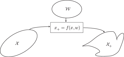
Figure 1: Set image of $\mathcal{X}$ with noise ​$w\in\mathcal{W}$ under map ​(1) .

Motivated by the computational complexity issues and the fact that deterministic formulations of the approximation problem may not be suitable in practical situations, in Dabbene et al. (2010) the authors proposed an original approach for tackling the problem, based on a probabilistic viewpoint. To this end, a probabilistic information over $\mathcal{X}$ and $\mathcal{W}$ is assumed to be known (which is actually the case in many applications), and an approximation $\mathcal{A}$ of $\mathcal{X_{+}}$ is deemed to be “good” if it contains all points in $\mathcal{X_{+}}$ with high probability. More formally, we assume that the sets $\mathcal{X}$ and $\mathcal{W}$ are endowed with probability measures $\mu_{\mathcal{X}}$ and $\mu_{\mathcal{W}}$. Then, for a given reliability level $\varepsilon$, the following concept of $\varepsilon$-probabilistic approximation is introduced.

Definition 1 ($\varepsilon$-probabilistic approximation of $\mathcal{X_{+}}$)

The

set $\mathcal{A}$ is an $\varepsilon$-probabilistic approximation of the set $\mathcal{X_{+}}$ if

$$\mathrm{Viol}(\mathcal{A})\leq\varepsilon,$$

with

$$\mathrm{Viol}(\mathcal{A}) \doteq \mathrm{Pr}\bigl{\{}x\in\mathcal{X},w\in\mathcal{W}\colon\,x_{+}=f\bigl{(}x,w\bigr{)}\not\in\mathcal{A}\bigr{\}}$$ (2)

$$= \int_{\mathcal{X_{+}}\setminus\mathcal{A}}f(x,w)\mathrm{d}\mu_{\mathcal{X}}(x)\mathrm{d}\mu_{\mathcal{W}}(w).$$

Note that the probability in (2) is measured with respect to the underlying measures $\mu_{\mathcal{X}}$ and $\mu_{\mathcal{W}}$. The left-hand side of the equation is referred to as the violation probability of the set $\mathcal{A}$.

The main characteristic of this approach is that an $\varepsilon$-probabilistic approximating set has neither to cover nor to be fully contained in $\mathcal{X}$; it just has to guarantee that the violation probability of the set $\mathcal{A}$ is bounded by $\varepsilon$. Clearly, we are interested in finding the smallest among such sets. In the sequel, we first define the two families of approximating sets considered in this paper.

2.1 Convex approximating sets: Ellipsoids, parallelotopes, and hyperrectangles

The following general description of the norm-based approximating set (NAS) was introduced in Dabbene et al. (2010):

$$\mathcal{A}(c,P)\doteq\left\{x\!\in\!{{\mathbb{R}}^{n}}\colon\,\|P(x-c)\|_{p}\leq\!1,\,P\!=\!P^{\top}\!\succeq 0\right\}.$$ (3)

Note that the family of sets above is parameterized by the positive-definite shape matrix $P$, and by the center $c\in{{\mathbb{R}}^{n}}$; it represents a generalization of the classical ellipsoidal set for norms different from the Euclidean one.

Indeed, for $p=2$, we obtain the ellipsoid

$$\mathcal{E}(c,P)\doteq\left\{x\in{{\mathbb{R}}^{n}}\colon\,x=c+P^{-1}z,\,\|z\|_{2}\leq 1\right\},$$

and for $p=\infty$ we get a so-called elementary parallelotope, a special-type polytope with parallel faces (these can be viewed as a particular class of zonotopes (Alamo et al., 2005) with positive definite generator matrix). In particular, if $P$ is chosen to be diagonal, we obtain a classical hyper-rectangle.

It follows that, in general, the problem of finding the minimum volume NAS containing $\mathcal{X_{+}}$ can be rewritten in the form of the following robust convex problem:

$$\begin{array}[]{l}\displaystyle{\min_{P,c}}\log\det(P^{-1})\\ ~{}~{}~{}~{}~{}\mbox{s.t.}~{}~{}~{}P=P^{\top}\succ 0,\\ ~{}~{}~{}~{}~{}~{}~{}~{}~{}~{}~{}~{}\|Px_{+}-c\|_{p}\leq 1\;\forall x_{+}\in\mathcal{X_{+}}.\end{array}$$ (NAS-robust)

2.2 Nonconvex approximations: Polynomial superlevel sets

In Dabbene and Henrion (2013), nonconvex set approximations based on the superlevel set of a multidimensional polynomial have been introduced, and shown to represent a simple and efficient way for describing complex shaped sets. Formally, assume we are given a compact semialgebraic set

$$\mathcal{S}:=\{x\in{\mathbb{R}}^{n}:b_{i}(x)\geq 0,\>i=1,2,\ldots,m_{b}\}$$

such that $\mathcal{X_{+}}\!\subseteq is$, with $b_{i}(x)$ being given polynomials (the set $\mathcal{S}$ is usually a hyper-rectangle). Then, given a polynomial of degree $\sigma\!>0$, i.e., $q\in\mathbb{P}_{\sigma}$, its polynomial superlevel set $\mathcal{U}(q)$ is defined as

$$\mathcal{U}(q)\doteq\{x\in\mathcal{S}:q(x)\geq 1\}.$$

In the sequel, we will refer to this family of sets as polynomial-based approximating sets (PAS). The goal is then to find a polynomial $q\in\mathbb{P}_{\sigma}$ whose corresponding PAS $\mathcal{U}(q)$ contains $\mathcal{X_{+}}$ and has minimal volume. In Dabbene and Henrion (2013), the following problem was formulated:

$$\begin{array}[]{rcll}&&\displaystyle{\min_{q\in\mathbb{P}_{\sigma}}}\!\!\!&\!\|q\|_{1}\\ &&\mathrm{s.t.}&q\geq 0\>\>\mathrm{on}\>\>\mathcal{S},\\ &&&q\geq 1\>\>\mathrm{on}\>\>\mathcal{X_{+}},\end{array}$$ (4)

and the $L^{1}$ measure above was shown to be a good surrogate to the volume of the set $\mathcal{U}(q)$. Moreover, theoretically rigorous convergence results were provided in Dabbene and Henrion (2013), showing that, if $\mathcal{X_{+}}$ is semialgebraic, a hierarchy of outer approximations obtained by solving the above problem for increasing values of $\sigma$ converges in volume (or, equivalently, almost uniformly) to the set $\mathcal{X_{+}}$.

We now make the important observation that this result still holds for generic compact sets, not necessarily of semialgebraic form. Hence, we propose the following family of PASs, where we further relax the positivity requirement of $q$ over $\mathcal{S}$ by requiring that the polynomial can be expressed as a sum-of-squares (SOS) over $\mathcal{S}$:

$$\begin{array}[]{rcll}&&\displaystyle{\min_{q\in\mathbb{P}_{\sigma}}}\!\!\!&\!\int_{\mathcal{S}}q(x)\,dx\\ &&\mathrm{s.t.}&q(x_{+})\text{~{}~{}~{}is SOS over }\mathcal{S},\\ &&&q(x_{+})\geq 1\quad\forall x_{+}\in\mathcal{X_{+}}.\end{array}$$ (PAS-robust)

Note that the requirement that $q$ is SOS over $\mathcal{S}$ can be formulated using Putinar’s Positivstellensatz and a hierarchy of finite-dimensional convex LMI relaxations which are linear in the coefficients of $q$. More specifically, we write $q=r_{0}+\sum_{i}^{m}r_{i}b_{i}$, where $r_{0},r_{1},\ldots,r_{m}$ are polynomial sum-of-squares of given degree $\sigma_{r}$, to be found. For simplicity, we choose $\sigma_{r}=\sigma$. For each fixed degree, the problem of finding such polynomials is an LMI; e.g., see (Lasserre, 2015, Section 3.2). Note again that problem (PAS-robust) is a robust convex program (that is, for every fixed $x_{+}$, we get a convex program).

3 Randomized approximations

In this section, we propose a simple randomized algorithm to construct, with arbitrarily high probability, $\varepsilon$-probabilistic approximations of the image set $\mathcal{X_{+}}$. The suggested randomized procedure is rather straightforward: We draw $N$ samples of $x\in\mathcal{X}$ according to the measure $\mu_{\mathcal{X}}$, obtaining the multisample

$$\left.x\right|_{1}^{N}\doteq\{x^{(1)},\dots x^{(N)}\}$$ (5)

and, similarly, we draw $N$ instances of the random noise $w\in\mathcal{W}$, drawn according to the (given) noise measure $\mu_{\mathcal{W}}$

$$\left.w\right|_{1}^{N}\doteq\{w^{(1)},\dots w^{(N)}\}.$$ (6)

Based on these samples, we compute the points

$$x_{+}^{(i)}=f(x^{(i)},w^{(i)}),\quad i=1,\ldots,N.$$

Then, we construct the approximating set $\mathcal{A}$ as the minimum-size bounding set containing the random points $\left.x_{+}\right|_{1}^{N}$ thus obtained. This is doable by solving one of the following two scenario problems:

$$\begin{array}[]{l}{\mathcal{A}}_{\rm NAS}\,\doteq\,\arg\displaystyle{\min_{P,c}}\displaystyle\log\det(P^{-1})\\ ~{}~{}~{}~{}\mbox{s.t.}~{}~{}P=P^{\top}\succ 0,\\ ~{}~{}~{}~{}~{}~{}~{}~{}~{}\|Px_{+}^{(i)}-c\|_{p}\leq 1,\;i=1,\ldots,N\end{array}$$ (NAS-random)

and

$$\begin{array}[]{l}{\mathcal{A}}_{\rm PAS}\,\doteq\,\arg\displaystyle{\min_{q\in\mathbb{P}_{\sigma}}}\displaystyle\int_{\mathcal{S}}q(x)\,dx\\ ~{}~{}~{}~{}\mathrm{s.t.}~{}~{}~{}q(x_{+})\text{~{}~{}~{}is SOS over }\mathcal{S},\\ ~{}~{}~{}~{}~{}~{}~{}~{}~{}~{}~{}q(x_{+}^{(i)})\geq 1,\;i=1,\ldots,N.\end{array}$$ (PAS-random)

The idea at the basis of the approach is depicted in Fig. 2, where random samples of $x$ and $w$ are drawn and mapped via the nonlinear function $f(\cdot,\cdot)$. Then, an approximation of $\mathcal{X_{+}}$ is obtained by constructing a minimum volume approximating set around these points.

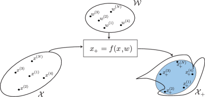
Figure 2: Randomized approximation of the image set.

Note that both problems above represent simple convex optimization problems which can be efficiently solved by available SDP solvers. In particular: (a) problem (NAS-random) reduces to a linear program (LP) for $p=1$ and diagonal $P$; (b) the constraints $q(x_{+}^{(i)})\!\geq\!1$ in problem (PAS-random) can also be expressed as an LP in the coefficients of $q(x)$. The procedure is summarized in the following algorithm.

Algorithm 1 ​Randomized Image Set ​ Approximation

0:  $\mathcal{X}$,

0:  ${\mathcal{A}}_{\rm NAS}$ (or ${\mathcal{A}}_{\rm PAS}$)

1:  draw $x^{(1)},\ldots,x^{(N)}$ over $\mathcal{X}$ and $w^{(1)},\ldots,w^{(N)}$ over $\mathcal{W}$

2:  construct $x_{+}^{(i)}=f(x^{(i)},w^{(i)}),\quad i=1,\ldots,N$

3:  solve problem (NAS-random) (or (PAS-random))

4:  return ${\mathcal{A}}_{\rm NAS}$ (or ${\mathcal{A}}_{\rm PAS}$).

The key features of the algorithm above are as follows: (i) there is no need in knowing the probability measures $\mu_{\mathcal{X}}$ and $\mu_{\mathcal{W}}$ explicitly, only the capability of obtaining random samples from these are mandatory for running the algorithm; (ii) formal results on the probabilistic quality of the obtained approximations are available. In particular, the properties of the algorithm follow from the well-known results of Calafiore and Campi (2006) on the so-called scenario optimization, which allow to bound a priori (before the algorithm is run) the violation probability of the solution.

Theorem 1

Let $\mathcal{A}$ (i.e., ${\mathcal{A}}_{\rm NAS}$ or ${\mathcal{A}}_{\rm PAS}$) be the outcome of Algorithm 1. Fix a risk level $\varepsilon>0$ and let $d$ be the “size” of the optimization problem NAS-random (or PAS-random). Then we have

$$\Pr\bigl{\{}\!\mathrm{Viol}({\mathcal{A}})\!>\!\varepsilon\!\bigr{\}}\leq\Phi(\varepsilon,N)\doteq\sum_{j=0}^{d-1}\!{\!N\choose{j}\!}\varepsilon^{j}(1\!-\!\varepsilon)^{N-j}.$$ (7)

Moreover, the above bound is tight, see Campi and Garatti (2008); Calafiore (2010).

Note that the result above makes explicit use of the size $d$ of the convex problem. This represents the number of free variables in the convex optimization problem; see Table 1.

Table 1: Number of design variables

Approximating set	Number of design variables
NAS - Ellipsoid/Parallelotope	$d=\frac{n(n+1)}{2}+n$
NAS - Hyperrectangle	$d=2n$
PAS - polynomial of degree $\sigma$	$d={n_{x}\choose{n_{x}+\sigma}}$

In order to obtain an expression for the desired sample size $N$ (the number of samples ensuring that the designed approximation is $\varepsilon$-optimal with probability at least $\delta$), we need to invert equation (7). The best bound currently available is proposed in Alamo et al. (2015), where it is shown that, given $\varepsilon,\delta\in(0,1)$, if $N$ is chosen as

$$N\geq\frac{e}{e-1}\frac{1}{\varepsilon}\left(d+\ln\frac{1}{\delta}\right),$$

then $\mathcal{A}$ is an $\varepsilon$-probabilistic approximation of $\mathcal{X_{+}}$ with probability at least $(1-\delta)$.

3.1 Numerical Example

To show the approximating sets obtained by Algorithm 1, we consider the nonlinear mapping

$$x_{+}(1) = \sin x(2)+3\cos x(2)+w(1),$$

$$x_{+}(2) = 3x(1)-20\log\bigl{(}1+x(2)\bigr{)}+w(2),$$ (8)

where $x\sim{{\lambda}}_{\mathcal{X}}$ with $\mathcal{X}=[0,1]^{2}$ and $w\sim{{\lambda}}_{\mathcal{W}}$ with $\mathcal{W}=[-0.2,0.2]^{2}$. Figure 3 depicts $N=200$ randomly generated points in $\mathcal{X_{+}}$, and the corresponding NAS and PAS probabilistic approximations. The shaded area represents the “true” set $\mathcal{X_{+}}$ obtained by generating one million points in it. These approximations are indeed seen to be neither inner nor outer ones.

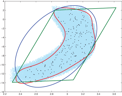
Figure 3: Image set of (3.1), with ellipsoidal NAS (blue), parallelotopic NAS (green), and PAS (red) approximations.

4 Randomized Filtering

The results of the previous sections are here reinterpreted in a filtering setting. The idea is rather intuitive: One can apply the image set description in an iterative way and use the approximation as a description of the state position at time $k$. For the sake of simplicity, we limit our exposition to the case where NAS descriptions are employed.

Consider the following discrete-time (autonomous) nonlinear system

$$x_{k+1} = f\bigl{(}x_{k},w_{k}\bigr{)},$$ (9)

$$y_{k} = g\bigl{(}x_{k}\bigr{)}+v_{k},$$ (10)

Equation (9) represents the systems dynamics, and $x_{k}$, $x_{k+1}\in{{\mathbb{R}}^{n}}$ denote the state at time instants $k$ and $k+1$, respectively, while $w_{k}\in{{\mathbb{R}}^{n_{w}}}$ is a noise vector, usually referred to as process noise. Equation (10) represents a nonlinear measurement mapping associated with the system equations, where $y_{k}\in{{\mathbb{R}}^{n_{y}}}$ is the measurement vector and $v_{k}\in{{\mathbb{R}}^{n_{v}}}$ is the measurement noise vector.

Various approaches have been adopted in the literature to address the filtering problem for this type of systems. In the Extended Kalman filtering approach, and, in general, in all the subsequently developed Gaussian Filtering techniques, (e.g., see Ito. and Xiong (2000)), probabilistic information on the states and noise is considered. The main approximation made in this setup is that all information about the state and noise is collected in the first two moments of this distribution; in other words, the state and (update and measurement) noise can be described by a Gaussian distribution. Note that, even if at $k=0$ everything could indeed be Gaussian, this is clearly not true after the first step, since Gaussian distributions are generally not preserved under nonlinear mappings. Approaches of this line are also those based on Unscented Kalman Filtering,  e.g., see Sarkka (2007).

A philosophically different approach is the one based on set-valued filtering, in which no probabilistic assumptions are made on the nature of the noise and on the a priori information on $x$; instead, a so-called unknown-but-bounded approach is used. In those works (e.g., see Calafiore (2005)), the a priori information is given in terms of a bounded set where the initial state is guaranteed to lie, and at each time step both process and measurement noise are assumed to take values from given bounded sets. Then, all information on the predicted state is itself captured by a set (usually an ellipsoid) which is guaranteed to contain the state at time $k+1$.

In this work, we propose a rapprochement between those two models and assume that the process and measurement noise are random, with given distributions over bounded support sets. That is, we assume that, at each time instant $k$, $w_{k}\in\mathcal{W}$ and $v_{k}\in\mathcal{V}$, where $\mathcal{W},\mathcal{V}$ are bounded sets. Moreover, we assume that $w_{k}$ has stochastic nature, and we denote by $\mathcal{P}_{\mathcal{W}}$ the probability measure on $\mathcal{W}$. Note that no stochasticity assumption is made on $v_{k}$.

The next approximation is crucial in our setup, and, from the philosophical point of view, it plays the same role of the Gaussian approximation commonly made in Gaussian filtering, in which the first two moments of the distribution are taken as representatives of the whole pdf of the propagated state.

Approximation 1 (State description)

At time $k$, all state information is captured by a NAS set $\mathcal{A}_{k}=\mathcal{A}(P_{k},c_{k})$ (e.g., an ellipsoid) with center $c_{k}$ and shape matrix $P_{k}$. Moreover, we assume that $x_{k}$ has stochastic nature, and it is uniformly distributed over $\mathcal{A}_{k}$.

Note again that this constitutes one of the main approximations introduced in our setup: At each step we ‘reset’ the density information about the state and make the implicit assumption that $x_{k}$ has a uniform distribution $\lambda$ with ellipsoidal support $\mathcal{A}_{k}$.

4.1 Probabilistically Guaranteed Simulation

In this section, we concentrate on the state dynamics equation only and propose a prediction filter for simulating the behavior of system (9). To this end, assume that at step $k$, the state $x_{k}$ is guaranteed (in probability) to lie inside a NAS set, that is $x_{k}\in\mathcal{A}_{k}\doteq\mathcal{A}(x_{k},P_{k}).$ Then, we can apply the set image approximation algorithm; namely, given a probabilistic parameter $\varepsilon$, we choose $N$ so as to guarantee a desired approximation level, and we start by drawing uniform random samples $x_{k}^{(1)},\ldots,x_{k}^{(N)}\sim{{\lambda}}_{\mathcal{A}_{k}}$, and $N$ noise samples $w_{k}^{(1)},\ldots,w_{k}^{(N)}\sim{{\lambda}}_{\mathcal{W}}$. Based on these samples, we compute the points $x_{k+1}^{(i)}=f(x_{k}^{(i)},w_{k}^{(i)})$, $i=1,\ldots,N$, and solve the NAS-random problem. The proposed procedure is summarized in Algorithm 2.

Algorithm 2 One-step Randomized Prediction Filter

0:  $\mathcal{A}_{k}$,

0:  $\mathcal{A}_{k+1}$

1:  draw $x_{k}^{(1)},\ldots,x_{k}^{(N)}\sim{{\lambda}}_{\mathcal{A}_{k}}$ and $w_{k}^{(1)},\ldots,w_{k}^{(N)}\sim{{\lambda}}_{\mathcal{W}}$

2:  construct $x_{k+1}^{(i)}=f(x_{k}^{(i)},w_{k}^{(i)}),\quad i=1,\ldots,N$

3:  solve problem NAS-random

4:  return $\mathcal{A}_{k+1}$.

Remark 1 ($m$-step ahead prediction)

The iterative one-step prediction scheme discussed above has been introduced having in mind the prediction-correction scheme that we formulate in the next section. However, there are cases when it could be convenient to directly perform an $m$-step ahead prediction, in one shot. To do this, a simple solution is to “propagate” the state samples $m$-times ahead in the following way: Generate $N$ samples $x_{k}^{(i)}$, $i=1,\ldots,N$, and $mN$ samples of uncertainty $w_{k+j-1}^{(i)}$, $i=1,\ldots,N$, $j=1,\ldots,m$, and iteratively compute

$$x_{k+j}^{(i)}=f(x_{k+j-1}^{(i)},w_{k+j-1}^{(i)}),\quad i=1,\ldots,N;\,j=1,\ldots,m.$$

Then, we can directly construct a NAS approximation of $\mathcal{A}_{k+m}$ based on the multisample $x_{k+m}^{(1)},\ldots,x_{k+m}^{(N)}$.

4.2 Measurement update

If a measurement is available, it can be immediately used to reject incorrect predictions, as discussed in Algorithm 3 (RPCF) below.

Algorithm 3 One-step Randomized Prediction-Correction Filter​ (RPCF)

0:  $\mathcal{A}_{k}$,

0:  $x_{k+1}$

1:  draw $x_{k}^{(1)},\ldots,x_{k}^{(N)}\sim{{\lambda}}_{\mathcal{A}_{k}}$ and $w_{k}^{(1)},\ldots,w_{k}^{(N)}\sim{{\lambda}}_{\mathcal{W}}$

2:  construct $x_{k+1}^{(i)}=f(x_{k}^{(i)},w_{k}^{(i)}),\quad i=1,\ldots,N$

3:  construct $z_{k+1}^{(i)}=y_{k+1}-g(x_{k+1}^{(i)}),\quad i=1,\ldots,N$

4:  if $z_{k+1}^{(i)}\not\in\mathcal{V}_{k}$ then

5:     reject $x_{k+1}^{(i)}$

6:  end if

7:  solve problem NAS-random

8:  return $\mathcal{A}_{k+1}$.

Remark 2 (Similarities with particle filtering)

In the so called particle filtering, particles are generated and fed through the dynamical system. Then, they are kept/discarded based on Bayesian-type reasonings. Our setup has strong similarities. Indeed, one can construct a “particle-like” implementation of the predictor-corrector randomized algorithm, where at each step not all samples are generated again, but instead, the non-discarded ones are fed through. This algorithm seems to provide a good practical behavior. However, it still needs a thorough theoretical analysis, which will be the subject of future work.

5 Numerical Example

As a filtering example, we tested the specific two-dimensional nonlinear system with scalar measurements, borrowed from Alamo et al. (2008), which was considered in the context of set filtering by means of zonotopic approximation sets:

$$x_{k+1}(1) = -0.7x_{k}(2)+0.1x_{k}(2)^{2}+0.1x_{k}(1)x_{k}(2)+0.1{\rm e}^{x_{k}(1)}+w_{k}(1),$$ (11)

$$x_{k+1}(2) = x_{k}(1)+x_{k}(2)-0.1x_{k}(1)^{2}+0.2x_{k}(1)x_{k}(2)+w_{k}(2),$$ (12)

$$y_{k} = x_{k}(1)+x_{k}(2)+v_{k},$$ (13)

where the propagation noise is $|w_{k}(1)|\leq 0.1$, $|w_{k}(2)|\leq 0.1$; the measurement error is $|v_{k}|\leq 0.2$, $k>0$; the initial state belongs to the box $\mathcal{X}_{0}=[-3,\,3]\times[-3,\,3]$. Note that the measurements are linear in both $x$ and $v$, and the dynamics is linear in $w$.

To shape the experiment, we first generated a “realized” trajectory $x^{sim}_{k}$ and the respective sequence of measurements $y_{k}$, $k=1,\dots,K$. Then, given $\mathcal{A}_{k}$ at step $k$, we sample $N$ points in $\mathcal{A}_{k}$ and propagate them via (11)–(12) to obtain a set $\tilde{\mathcal{X}}_{k}$ of candidate next-step points $x^{(i)}_{k+1}$. We call $x^{(i)}_{k+1}\in\tilde{\mathcal{X}}_{k}$ good if it fits the measurement, i.e.

$$|y_{k+1}-x_{k+1}^{(i)}(1)-x_{k+2}^{(i)}(2)|\leq 0.2,$$ (14)

see (13). We call this account for the measurements as correction step or rejection (of bad points). Because of the linearity of the measurements, the good points are those who fall in the slab $\mathcal{S}_{k+1}$ defined by (14).

Next, we build a minimum volume set $\mathcal{A}_{k+1}$ (of the shape adopted) that contains only the good points and adopt it as a probabilistic approximation set for $x_{k+1}$.

Figure 4 represents the evolution of the sets $\mathcal{A}_{k}$ in the case of ellipsoidal shapes (the circle represents the ellipse $\mathcal{E}([0.6,0.07]^{\top},6.8I)$ of initial uncertainty). The stars correspond to the reference trajectory $x^{sim}_{k}$.

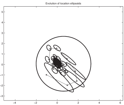
Figure 4: Evolution of the approximation ellipses.

For the same realization we plot $\log\bigl{(}\mathrm{vol}(\mathcal{A}_{k})\bigr{)}$, see Fig. 5 (left). We remark that this quantity is of the same order of magnitude (or better) than that for the zonotopes in Alamo et al. (2008), but of course the computations are way simpler, and this advantage will get stronger as the dimension of $x$ grows.

 

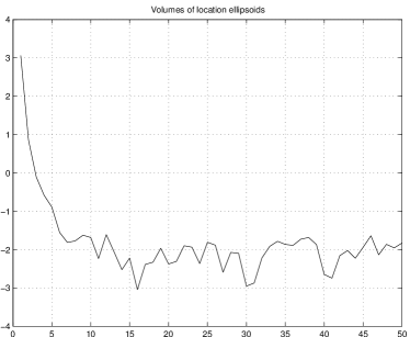
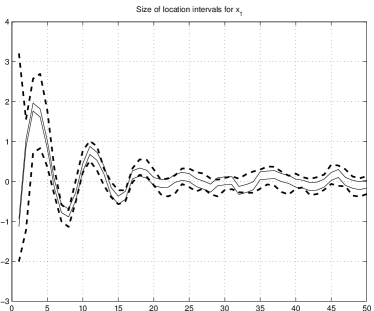
Figure 5: The volumes of the approximation ellipsoids (left) and estimation error for $x^{sim}_{1}(k)$ (right).

The filtering goal was to estimate $x_{k}(1)$, the first component of $x_{k}$. In Fig. 5 (right), we plot the $x(1)$-span of our ellipses, representing the estimation error, (bold dashed curves), while with the solid line we plot the worst-case bounds on $x(1)$ obtained from the reference trajectory: $x^{sim}_{k}(1)\pm 0.1$ (see definition (11)–(12) keeping in mind that the bounded propagation noise $|w_{k}(1,2)|\leq 0.1$ enters additively in the dynamics).

Notice that sometimes the inner corridor goes outside the bounds obtained by our method. This is exactly what illustrates the nature of our approach: We do neglect low-probability events.

Remark 3 (Comments on re-sampling and re-use)

In the RPCF Algorithm, many samples could be rejected due to the measurement equation. Experiments seem to show that in such cases it is preferable to re-sample the samples rejected in the measurement phase, so as to guarantee that the new set $\mathcal{A}_{k+1}$ is constructed based on a sufficiently large number of samples. Another point worth noticing is that, on the contrary, having built the $\mathcal{A}_{k}$ at step $k$, we already possess $N_{good}\leq N$ points inside it, so that they can be re-used (propagated), and just the rest $N-N_{good}$ ones are to be newly sampled; this is called re-use.

6 Conclusions

We developed an efficient algorithm for constructing $\varepsilon$-probabilistic approximations of the image set of a noisy nonlinear mapping. The recursive application of such technique, combined with an ad-hoc rejection procedure, leads to the design of a new family of randomized prediction-correction filters, which showed themselves pretty competitive with both classical set-theoretical and Gaussian filtering methods. The derivations of the RCPF were limited to the NAS setting, but we stress that the use of PAS descriptions for the construction of prediction/correction filters is also possible in principle. However, we admit that in that case, the computations may become too cumbersome for online implementations.

References

- Alamo et al. (2005) T. Alamo, J.M. Bravo, and E.F. Camacho. Guaranteed state estimation by zonotopes. Automatica, 41(6):1035–1043, 2005.
- Alamo et al. (2008) T. Alamo, J.M. Bravo, M.J. Redondo, and E.F. Camacho. A set-membership state estimation algorithm based on DC programming. Automatica, 44(1):216–224, 2008.
- Alamo et al. (2015) T. Alamo, R. Tempo, A. Luque, and D.R. Ramirez. Randomized methods for design of uncertain systems: Sample complexity and sequential algorithms. Automatica, 52:160–172, 2015.
- Calafiore and Campi (2006) G. Calafiore and M. Campi. The scenario approach to robust control design. IEEE Transactions on Automatic Control, 51(5):742–753, 2006.
- Calafiore et al. (2011) G. Calafiore, F. Dabbene, and R. Tempo. Research on probabilistic methods for control system design. Automatica, 47:1279–1293, 2011.
- Calafiore (2005) G.C. Calafiore. Reliable localization using set-valued nonlinear filters. IEEE Transactions on Systems, Man, and Cybernetics, 35(2):189–197, 2005.
- Calafiore (2010) G.C. Calafiore. Random convex programs. SIAM Journal on Optimization, 20(6):3427–3464, 2010.
- Campi and Garatti (2008) M. Campi and S. Garatti. The exact feasibility of randomized solutions of robust convex programs. SIAM Journal on Optimization, 19:1211—1230, 2008.
- Dabbene and Henrion (2013) F. Dabbene and D. Henrion. Set approximation via minimum-volume polynomial sublevel sets. In Proc. of the European Control Conference, 2013.
- Dabbene et al. (2010) F. Dabbene, C. Lagoa, and P. Shcherbakov. On the complexity of randomized approximations of nonconvex sets. In Proc. IEEE Multiconference on Systems and Control, 2010.
- El Ghaoui and Calafiore (2001) L. El Ghaoui and G. Calafiore. Robust filtering for discrete-time systems with bounded noise and parametric uncertainty. IEEE Transactions on Automatic Control, 46(7):1084–1089, July 2001.
- Ito. and Xiong (2000) K. Ito. and K. Xiong. Gaussian filters for nonlinear filtering problems. IEEE Transactions on Automatic Control, 45(5):910–927, 2000.
- Lasserre (2015) J.B. Lasserre. Level sets and non Gaussian integrals of positively homogeneous functions. Int. Game Theory Review, 17(1), 2015.
- Nesterov and Nemirovski (1994) Y. Nesterov and A.S. Nemirovski. Interior Point Polynomial Algorithms in Convex Programming. SIAM, Philadelphia, 1994.
- Sarkka (2007) S. Sarkka. On unscented Kalman filtering for state estimation of continuous-time nonlinear systems. IEEE Trans. on Automatic Control, 52(9):1631–1641, 2007.
- Tempo et al. (2013) R. Tempo, G.C. Calafiore, and F. Dabbene. Randomized Algorithms for Analysis and Control of Uncertain Systems: With Applications. Springer, 2nd edition, 2013.
- Wojciechowski and Vlach (1993) J. M. Wojciechowski and J. Vlach. Ellipsoidal method for design centering and yield estimation. Transactions on Computer-Aided Design of Integrated Circuits and Systems, 12:1570–1579, 1993.