More on quantum kinks in gauge theories on $R^{2}\otimes S^{1}$

Abstract

Quantum kinks in gauge theories on $R^{2}\otimes S^{1}$ space-time are studied. To obtain the, explicit profile of the kinks, we calculated effective actions including derivative corrections for vacuum gauge fields on $S^{1}$ at zero, and finite temperature up to one-loop level. It is found that there are soliton solutions in scalar QED. We also find that the derivative correction tends to make the vacuum unstable in $SU(2)$ Yang-Mills theory.

1 Introduction

Gauge theories on space-times with non-trivial topologies have been investigated in the literature on Kahza-Klein theories and the low-energy superstring theories. The Wilson-line symmetry breaking is known as an alternative mechanism to break the gauge symmetry in such theories [1]. The vacuum expectation value for the gauge field on a compact space plays a role of a Higgs condensate in the mechanism.

Solitons in the space-time with non-trivial topology have recently been studied in connection with topological aspects of gauge theories. For QED on $R^{2}\otimes S^{1}$, Higuchi and Parker [3] have shown the existence of kink solutions, using an effective potential for vacuum gauge field at one-loop level.

Since the kinks are the spatially varying configuration of the vacuum gauge field, the derivative corrections to the action, which come from the loop effect, may become important. If one wish to study the properties of the quantum solitons, one should evaluate the derivative corrections to the effective action.

In this paper, we calculate the effective action for the vacuum gauge field, including the second-derivative corrections for scalar QED and $SU(2)$ Yang-Mills theory on $R^{2}\otimes S^{1}$ space-time and investigate the quantum soliton at one-loop level.

In sect. 2, we provide the effective action for the vacuum gauge field, which is induced by complex scalar fields and Dirac fermions on $R^{2}\otimes S^{1}$. In sect. 3, we show the explicit shape and the mass of the quantum kink in scalar QED on $R^{2}\otimes S^{1}$. The high-temperature case is examined in sect. 4. In sect. 5, we derive the second-derivative terms for the vacuum gauge field in $SU(2)$ Yang-Mills theory on $R^{2}\otimes S^{1}$. Section 6 is devoted to conclusion.

We reserve the explicit form of the one-loop corrections ($V$ and $\gamma$ in the text) to the appendix.

2 Effective action

The one-loop effective action is formally written as

$$\Gamma^{(1)}=\frac{1}{2}{\rm tr}\ln\Delta\,.$$ (1)

For a complex scalar coupled with a $U(1)$ gauge field on $R^{2}\otimes S^{1}$, the second-order differential operator $\Delta$ is taken as

$$\Delta=-\partial^{2}_{t}-\partial^{2}_{x}-(\partial_{y}\pm ie\langle A_{y}\rangle)^{2}\,,$$ (2)

where the coordinate $y$ corresponds to the compactified dimension and $e$ is the gauge coupling. We will work with the Euclidean signature for the metric. We will also introduce the dimensionless variable $\phi=eL\langle A_{y}\rangle$. We treat $\phi$ as a spatially ($x$-) dependent quantity.

To calculate the effective action for spatially dependent background, we adopt the method introduced by Moss, Toms and Wright [4]. The Green’s function at the zeroth order in the derivative expansion [4] in the momentum space is given by

$$G_{0}=(k^{2}+(2\pi l\pm\phi)^{2}/L^{2})^{-1}\,,$$ (3)

where $l$ is an integer, $L$ is the length of the circumference of $S^{1}$. Since further procedure to obtain the derivative corrections to the effective action is similar to the way used by Moss, Toms and Wright [4], we will not repeat it here. We note however that there is a large difference in the manner of taking the trace with respect to the momentum space, because of the intertwining between vacuum gauge field $\phi$ and the discrete momentum on $S^{1}$.

We consider the $U(1)$ gauge theory coupled to $N$ ‘copies’, of complex scalar fields. The Lagrangian for this case is

$$L_{\mbox{scalar QED}}=\frac{1}{4}F^{\mu\nu}F_{\mu\nu}+\sum_{i=1}^{N}\left|\left(\partial_{\mu}-i\frac{e}{\sqrt{N}}A_{\mu}\right)\Phi^{i}\right|^{2}+m^{2}\left|\Phi^{i}\right|^{2}\,,$$ (4)

where $F_{\mu\nu}=\partial_{\mu}A_{\nu}-\partial_{\nu}A_{\mu}$ and $m$ is the mass of the complex scalar fields.

If we rewrite

$$\phi(x)\equiv\frac{e}{\sqrt{N}}L\langle A_{y}\rangle\,,$$ (5)

the classical action for $\phi$ becomes

$$\Gamma^{(0)}=N\int d^{3}x\frac{1}{2}\frac{1}{e^{2}L^{2}}(\partial_{x}\phi)^{2}\,.$$ (6)

Obviously, the one-loop effective action is expressed with an overall factor $N$. Since the two- and higher-loop correction is at most order $O(N^{0})$ only the classical and the one-loop action are effective in the limit $N\rightarrow\infty$.

Because of the coupling dependence in (6) and the one-loop potential which is proportional to $L^{-3}$, the typical scale for the ‘thickness’ of the kink turns out to be $L/(e^{2}L)^{1/2}$. Therefore we may omit higher-derivative contribution to the kink if the dimensionless quantity $e^{2}L$ is sufficiently small. Here we consider only second-order derivative correction at one loop under the assumption $e^{2}L\ll 1$.

To avoid the repetition of $N$, we use the action ‘per one charged field’ from now on.

The effective potential for r from one-loop contribution of complex scalar field in massless limit can be found as

$$V(\phi)=\Gamma^{(1)}_{0}\large/\int d^{3}x=\frac{2}{\pi L^{3}}\sum_{l=1}^{\infty}\frac{\sin^{2}(l\phi/2)}{l^{3}}\,,$$ (7)

where we set the energy of the vacuum at $\phi=0$ (mod $2\pi$) to zero, since the vacuum energy independent of $\phi$ is irrelevant for our present purpose.

The second-derivative term induced by the massless scalar field is written as

$$\Gamma^{(1)}_{2}=\int d^{3}x\frac{1}{48\pi}{\rm cosec}^{2}\frac{\phi}{2}\,\frac{(\partial_{x}\phi)^{2}}{L}\equiv\int d^{3}x\frac{1}{2}\frac{\gamma(\phi)}{e^{2}L^{2}}(\partial_{x}\phi)\,.$$ (8)

The quantum effect from fermions is also calculated by a similar method. The effective potential induced by a single, massless Dirac fermion field is

$$V_{f}(\phi)=\frac{1}{\pi L^{3}}\sum_{l=1}^{\infty}\frac{\cos l\phi-(-1)^{l}}{l^{3}}\,,$$ (9)

and the second-derivative correction from a single, massless Dirac field is given by

$$\Gamma^{(1)}_{2,f}=\int d^{3}x\frac{1}{96\pi}{\rm cosec}^{2}\frac{\phi}{2}\,\frac{(\partial_{x}\phi)^{2}}{L}\,.$$ (10)

In the appendix, the general expressions for the one-loop effects of scalars and fermions with arbitrary masses at arbitrary temperature are found.

In the next section, we derive the kink solution in the presence of the derivative correction.

3 Quantum kinks

In this section we explicitly solve the one-loop modified action to obtain the kink solution. Now a short comment is in order. In pure $U(1)$ gauge + massless fermion system, the vacuum is located at $\phi=\pi$ (mod $2\pi$). Thus the topological soliton which interpolates two vacua must pass through $\phi=0$ (mod $2\pi$), where the second-derivative correction diverges. This exhibits the failure of the expansion of effective action in terms of the number of derivatives [5]. It is also said that the Green’s function in the momentum space has singularities or non-analytic points [6].

For a gauge system with complex scalar fields, the difficulty does not appear because the gradient of the field is rapidly reduced near $\phi=0$ for the ‘tail’ of the kink. We will evaluate the contribution of the higher order in the derivative expansion.

From now on, we consider the effective action from a scalar one loop. The effective action we now consider is

$$\Gamma=L\int_{-\infty}^{\infty}dx\left[\frac{1}{2}\frac{1+\gamma(\phi)}{e^{2}L^{2}}(\partial_{x}\phi)^{2}+V(\phi)\right]\,,$$ (11)

where $\gamma$ and $V$ are given by (8) and (7).

Here we want static solutions, and then we suppressed the integration by time variable, while we integrated out in terms of the coordinate $y$, in (11).

We can simplify the action by using the coordinate $z$ defined as

$$z\equiv\sqrt{e^{2}L}\frac{x}{L}\,,$$ (12)

and we get

$$\Gamma=\frac{1}{\sqrt{e^{2}L}L}\tilde{\Gamma}=\frac{1}{\sqrt{e^{2}L}L}\int_{-\infty}^{\infty}dz\left[\frac{1}{2}(1+\gamma(\phi))(\partial_{x}\phi)^{2}+\tilde{V}(\phi)\right]\,,$$ (13)

where $\tilde{V}(\phi)=L^{3}V(\phi)$.

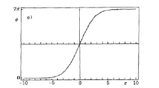
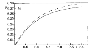
Figure 1: a) A view of a quantum kink. b) The solid line shows the kink in the system governed by the effective action (11). The dashed line shows the kink in the same system but where the derivative correction $\gamma$ is omitted.

The kink solution with the boundary conditions $\phi(-\infty)=0$ and $\phi(\infty)=2\pi$ can be easily obtained from this action. The shape of kink is shown in fig. 1a) for $e^{2}L=0.01$. To see the effect of derivative correction, we also show the kink for the system governed by the action (11) but without $y$. The difference in the profile is very small and thus a small portion of fig. 1a) is shown in fig. 1b) with an appropriate magnification. The solid line shows the piece of the kink in the system governed by the effective action (11), while the dashed line shows the kink in the same system but with the derivative correction $\gamma$ omitted.

The tail of the kink approaches the vacuum value as $z^{-1}$ in the presence of the second-derivative correction. Without the derivative correction, $\phi$ is damped exponentially near the vacua. The derivative correction makes the kink less steeper; nevertheless no singular behaviour is found, and thus the higher order in the derivative expansion is expected to be suppressed by the power of $e^{2}L$.

Figure 2: The kink mass in the cases with and without the derivative correction, as a function of $e^{2}L$. The solid line and dashed line correspond to the kink mass with and without the second-derivative correction. Note that the mass is scaled by $1/\sqrt{e^{2}L^{3}}$.

The mass of the kink $M$ is given by $\Gamma(\phi_{kink})$. The difference between the kink mass with and without the derivative correction as a function of $e^{2}L$ is shown in fig. 2. The derivative correction reduces the kink mass.

The mass of the kink is expressed approximately as

$$M=\frac{1}{\sqrt{e^{2}L^{3}}}(5.104+0.26e^{2}L)\,.$$ (14)

Note that this expression is derived for one massless complex scalar field. For $N$ scalar fields, the mass is the above result multiplied by $N$. It is a pleasure to point out that the leading term for the kink mass takes a very similar form as the monopole case, where the mass is given by the typical mass scale in the system divided by the absolute value of the gauge coupling.

4 Quantum kinks at finite temperature

Now, we consider the finite-temperature effect. First, we derive the effective action for r in the high-temperature limit. The effective potential which comes from the one-loop effect of a complex scalar field with mass m at high temperature $T$ ($\gg L^{-1}$) turns out to be

$$V_{high~{}T}(\phi)=\frac{4T}{\pi}\sum_{l=1}^{\infty}\frac{m}{Ll}K_{2}(mLl)\sin^{2}\frac{l\phi}{2}\,,$$ (15)

where $K_{2}$ is the modified Bessel function of the second kind and the term independent of $\phi$ is dropped. (See also the appendix.)

The correction to the kinetic term for r at high temperature is given by

$$\Gamma^{(1)}_{2,high~{}T}\frac{T}{8}\int d^{3}x\sum_{l=-\infty}^{\infty}\frac{(2\pi l+\phi)^{2}}{((2\pi l+\phi)^{2}+m^{2})^{5/2}}(\partial_{x}\phi)^{2}\,.$$ (16)

(See also the appendix.) The typical scale of the gradient of the kink configuration becomes $(e^{2}TL^{2})^{1/2}L$ at high temperature and small $m$, instead of $(e^{2}L)^{1/2}L$ at zero temperature.

The derivative correction makes the tail of kink longer in general. $\phi$ approaches the vacuum value as $x^{-1}$ in the limit of the infinitesimal mass for the scalar field, as the zero temperature case.

However, even if the kink solution exists, the mass of the kink diverges in the massless limit for the scalar field. This is due to the integration in the region of the long tail of the kink. The mass of the kink inflates for the case with the scalar field with small mass at high temperature, as $(T/m)^{1/2}$. The divergence may originate from the infrared behaviour of the field in the low-dimensional space.

5 Non-Abelian case

In this section, we consider the one-loop quantum effect of $SU(2)$ Yang-Mills field. The classical Lagrangian is given by

$$L_{YM}=\frac{1}{4}\sum_{a=1}^{3}(F^{a}_{\mu\nu})^{2}\,,$$ (17)

where the gauge field strength is defined as

$$F^{a}_{\mu\nu}=\partial_{\mu}A^{a}_{\nu}-\partial_{\nu}A^{a}_{\mu}-e\varepsilon^{abc}A_{\mu}^{b}A_{\nu}^{c}\,.$$ (18)

Then the kink consists of a component of the gauge field, say, $\langle A^{3}_{y}\rangle$.

We take the gauge-fixing term as

$$L_{g.f.}=\frac{1}{2\alpha}\sum_{a=1}^{3}(B^{a})^{2}\,,$$ (19)

with

$$B^{1} = \partial_{i}A_{i}^{1}+\alpha(\partial_{y}A_{y}^{1}+\langle A_{y}^{2}\rangle A_{y}^{2})+2U^{i}A_{i}^{1}\,,$$ (20)

$$B^{2} = \partial_{i}A_{i}^{2}+\alpha(\partial_{y}A_{y}^{2}-\langle A_{y}^{2}\rangle A_{y}^{1})+2U^{i}A_{i}^{2}\,,$$ (21)

$$B^{3} = \partial_{i}A_{i}^{3}+\alpha(\partial_{y}A_{y}^{3})+2U^{i}A_{i}^{3}\,,$$ (22)

where $A_{y}^{3}$ denotes the deviation from the background field, $i=\{t,x\}$ and $U_{x}=\partial_{x}\langle A_{y}^{3}\rangle(\langle A_{y}^{3}\rangle)^{-1}$. $\alpha$ is the gauge parameter we set to unity hereafter.

Combining (17) and (19), we find that the one-loop effective action is written in the form

$$\Gamma^{(1)}=\frac{1}{2}{\rm tr~{}}\ln\Delta_{YM}-{\rm tr~{}}\ln\Delta_{gh}\,,$$ (23)

where

$$\Delta_{YM}^{\mu\nu} = -\delta^{\mu\nu}(D_{\lambda})^{2}+2(U^{\mu}\partial^{\nu}-U^{\nu}\partial^{\mu})-[\partial^{\mu}U^{\nu}+\partial^{\nu}U^{\mu}]+U^{\mu}U^{\nu}\,,$$ (24)

$$\Delta_{gh} = -(D_{\lambda})^{2}-2U^{\mu}\partial_{\mu}\,.$$ (25)

Here the $SU(2)$ indices are suppressed and the covariant derivative is defined as

$$D_{i} = \delta^{ab}\partial_{i}\,,$$ (26)

$$D_{y} = \delta^{ab}\partial_{y}+e\varepsilon^{abc}\langle A_{y}^{c}\rangle\,.$$ (27)

$U_{y}\equiv 0$ is added as a dummy.

After the calculation is done similarly to ref. [4], we find the second-order derivative correction to the effective action for $\phi\equiv eL\langle A_{y}^{3}\rangle$ at one-loop order at zero temperature:

$$\Gamma^{(1)}_{2}=-\int d^{3}x\frac{11}{48\pi}{\rm cosec}^{2}\frac{\phi}{2}\frac{(\partial_{x}\phi)^{2}}{L}\,.$$ (28)

The sign of the above correction is the opposite sign of the classical term. Thus one may suspect the instability of the vacuum. The inclusion of the other matter field may ensure the stability. In addition, the two-loop contribution may be important (since one cannot argue for omission of the higher loops by large $N$, unlike the previous case for scalar fields), so we cannot declare a definite statement.

6 Conclusion and remarks

In the present paper we have studied quantum kinks in gauge theories on $R^{2}\otimes S^{1}$. Since the kink solutions should be treated as the spatially dependent background, we have calculated the effective action by the method introduced by Moss, Toms and Wright [4]. For scalar QED, the effective action has been calculated and the kink solution has been obtained numerically.

At high temperature, the kink mass diverges in the limit of the infinitesimal mass for the complex scalar field, though the kink solution exists. This fact may indicate the infrared problem in such a low-dimensional system.

For the pure $SU(2)$ Yang-Mills system, the possible instability of the gauge vacuum due to the derivative correction has been found. The instability can be cured by adding matter fields. Moreover, it is possible that the higher-loop effect may change the effective action largely.

We have presented an example in which the derivative correction has a sense in the calculable quantity (=kink mass). We have not yet known other examples for applications of the derivative correction to concrete calculation of physical quantities, though the importance of the derivative correction has been advocated in the literature on the cosmological phase transitions. It may be necessary to investigate the evaluation of the derivative correction by other methods than the expansion in terms of the number of the derivatives. We also study the singularity of the Green’s function in the momentum space in general.

Finally, we hope that the kink we have studied has some relevance to the low-dimensional physics.

APPENDIX A

In this appendix we exhibit the effective potential $V(\phi)$ and the second-derivative correction $\gamma(\phi)$ for the scalar and Dirac fields for the vacuum $U(1)$ gauge field as well as for the $SU(2)$ Yang-Mills field for the vacuum gauge field.

A) Complex scalar fields.

For a complex scalar field with mass $m$ at temperature $T$, we find

$$V(\phi)=\frac{\sqrt{2}m^{3}}{\pi^{3/2}}\left(\sum_{n=-\infty}^{\infty}\sum_{l=-\infty}^{\infty}\right)^{\prime}\frac{K_{3/2}(z_{nl})}{z_{nl}^{3/2}}\sin^{2}\frac{l\phi}{2}\,,$$ (29)

where $K_{3/2}(z)$ is the modified Bessel function of the second kind, $z_{nl}\equiv m\sqrt{(n/T)^{2}+(Ll)^{2}}$ and the prime on sums indicates that the term with $n=l=0$ is to be omitted. We also omit the vacuum energy which is independent of $\phi$.

And the second-derivative correction is found to be

$$\gamma(\phi)=\frac{e^{2}TL^{2}}{4}\sum_{n=-\infty}^{\infty}\sum_{l=-\infty}^{\infty}\frac{(2\pi l+\phi)^{2}}{[(2\pi TLn)^{2}+(2\pi l+\phi)^{2}+(mL)^{2}]^{5/2}}\,.$$ (30)

The results for massless fields at zero and high-temperature in the text are obtained by taking the limit $m\rightarrow 0$ and the corresponding limit on $T$.

B) Dirac fermion fields.

For a Dirac fermion field with mass $m$ at temperature $T$, we find

$$V_{f}(\phi)=\frac{m^{3}}{\sqrt{2}\pi^{3/2}}\left(\sum_{n=-\infty}^{\infty}\sum_{l=-\infty}^{\infty}\right)^{\prime}(-1)^{n}\frac{K_{3/2}(z_{nl})}{z_{nl}^{3/2}}(\cos l\phi-(-1)^{l})\,,$$ (31)

where $K_{3/2}(z)$ is the modified Bessel function of the second kind, $z_{nl}\equiv m\sqrt{(n/T)^{2}+(Ll)^{2}}$ and the prime on sums indicates that the term with $n=l=0$ is to be omitted. We also omit the vacuum energy which is independent of $\phi$.

And the second-derivative correction is found to be

$$\gamma_{f}(\phi)=\frac{e^{2}TL^{2}}{4}\sum_{n=-\infty}^{\infty}\sum_{l=-\infty}^{\infty}\frac{(2\pi TL(n+1/2))^{2}+(mL)^{2}}{[(2\pi TL(n+1/2))^{2}+(2\pi l+\phi+(mL)^{2}]^{5/2}}\,.$$ (32)

The results for massless fields at zero temperature in the text are obtained by taking the limit $m,T\rightarrow 0$.

C) $SU(2)$ Yang-Mills fields (at zero temperature).

For $SU(2)$ Yang-Mills fields at zero temperature, we find

$$V_{YM}(\phi)=\frac{2}{\pi}\sum_{l=1}^{\infty}\frac{1}{(Ll)^{3}}\sin^{2}\frac{l\phi}{2}\,,$$ (33)

where we omit the vacuum energy which is independent of $\phi$.

And the second-derivative correction at zero temperature is found to be

$$\gamma_{YM}(\phi)=-\frac{11e^{2}L}{24\pi}{\rm cosec}^{2}\frac{\phi}{2}\,.$$ (34)

References

- [1] Y. Hosotani, Phys. Lett. B126 (1983) 309; D. J. Toms, Phys. Lett. B126 (1983) 445; E. Witten, Nucl. Phys. B258 (1985) 75.
- [2] K. Lee, R. Holman and E. W. Kolb, Phys. Rev. Lett. 59 (1987) 1069; B.-H. Lee et al., Phys. Rev. Lett. 60 (1988) 2231; M. Tomiya, J. Phys. G14 (1988) L153.
- [3] A. Higuchi and L. Parker, Mod. Phys. Lett. A5 (1990) 2251.
- [4] I. Moss, D. Toms and A. Wright, Phys. Rev. D46 (1992) 1671.
- [5] S. G. Naculich, Phys. Rev. D46 (1992) 5487; S. Dodelson and B.-A. Gradwohl, Nucl. Phys. B400 (1993) 435.
- [6] P. Elmfors, K. Enqvist and I. Vilja, Nucl. Phys. B422 (1994) 521.