2-D studies of Relativistic electron beam plasma instabilities in an inhomogeneous plasma

Abstract

Relativistic electron beam propagation in plasma is fraught with several micro instabilities like two stream, filamentation etc., in plasma. This results in severe limitation of the electron transport through a plasma medium. Recently, however, there has been an experimental demonstration of improved transport of Mega Ampere of electron currents (generated by the interaction of intense laser with solid target) in a carbon nanotube structured solid target [Phys. Rev Letts. 108, 235005 (2012)]. This then suggests that the inhomogeneous plasma (created by the ionization of carbon nano tube structured target) helps in containing the growth of the beam plasma instabilities. This manuscript addresses this issue with the help of a detailed analytical study and simulations with the help of 2-D Particle - In - Cell code. The study conclusively demonstrates that the growth rate of the dominant instability in the 2-D geometry decreases when the plasma density is chosen to be inhomogeneous, provided the scale length $1/k_{s}$ of the inhomogeneous plasma is less than the typical plasma skin depth ($c/\omega_{p0}$) scale. At such small scale lengths channelization of currents are also observed in simulation.

I Introduction

The relativistic beam plasma system occurs in the context of many frontier research areas in both laboratory and space plasmas, such as the fast ignition scheme of inertial confinement fusion tabak_05 , compact particle accelerators malka , solar flares physics solarflare , cosmic magnetic field generation cosmaggen and magnetic field reconnection s_bulnov . Therefore, the study of instabilities associated with the relativistic beam-plasma systems is of central importance in understanding issues pertaining to a better transport of beam electrons in the plasma and provide clues to improve upon it. The manuscript explores this in detail.

When a short, intense laser pulse (I$\geq 10^{19}$W/$cm^{2}$) irradiates a solid target, a relativistic electron beam is generated through the process of wave breaking Modena ; malka ; joshi . This relativistic electron beam can propagate inside the plasma target even when the current associated with it exceeds the Alfven current limit $I=(mc^{3}/e)\gamma=17{\gamma_{b}}$ kA, here $m$ is the electron mass, $e$ is the electronic charge, $c$ is speed of light and $\gamma_{b}$ is the Lorentz factor of the beam. This is because simultaneously a return current is induced by the electrons of the background plasma which compensates the forward beam electron current. This combination of forward and return current is, however, highly unstable to two stream and filamentation instabilities. For the two stream (longitudinal mode) bhom instability, the perturbations propagate parallel to the direction of the beam flow. When the perturbations propagate normal to the beam propagation direction they are termed as the filamentation instability (transverse mode) fried ; lee . This is also often known as the Weibel instability weibel .

In the general case the perturbation would propagate in a direction oblique to the beam and would have both filamentation and two stream characteristics. The instabilities associated with the obliquely propagating perturbations have been investigated in the cold fluid limit Taguchi as well as by kinetic approaches kinetic . The particle-in-cell (PIC) simulations Dieckmann ; shukla have been carried out to validate the results. It has been shown that when $\gamma_{b}>1$, relativistic effects come in to play and the filamentation instability dominates over the two-stream instability bret . A full hierarchical map showing the parameter regions (ratio of the beam density to the plasma density and $\gamma_{b}$) where these modes dominate has been provided in review . The maximally growing mode amongst the spectrum of unstable modes determines the beam evolution and sets the stage for the subsequent non-linear evolution. In fact the magnetic field generation is also closely linked with these modes and occurs due to the current imbalance created by the most dominant modes of the instability. As the amplitude of the perturbations increase the nonlinear coupling defines the spectral cascade to other scales making the magnetic power spectrum turbulent in many scenarios. This in turn is detrimental to beam transport.

There are many attempts at avoiding and/or suppressing such instabilities with are responsible for current separation. For instance, theoretical and experimental work on collimated propagation of electron beam assisted by resistivity gradient have been reported in Ref. A.R.BELL ; B.RAMA . A recent experiment g.r.k has demonstrated transport of Mega Amperes of electron currents through nano structured target over distances of the order of millimeter. The transportation of electron beam over such distances is possible only if the beam plasma associated instabilities are somehow suppressed and the separation between forward and return currents does not take place as rapidly as predicted by the growth rate of these instabilities. In a simplified 1-D treatment, the suppression of Weibel/filamentation instability by the equilibrium density inhomogeneity (due to the nanostructures) has been shown in some recent studies mishra ; chandra . However, for the parameters of experimental system g.r.k , typically the oblique mode would be the fastest growing mode review . This necessitates a 2-D treatment wherein the role of plasma inhomogeneity on the growth of oblique mode should be investigated. Such a study is the main objective of the work presented in this manuscript.

We have carried out the linear analysis of the beam plasma instability in an inhomogeneous plasma medium by using the coupled Maxwell and two-fluid electron equations in the relativistic regime. The inhomogeneity in the beam-plasma density has been chosen to have a sinusoidal profile orthogonal to the direction of the beam propagation. This inhomogeneous density mimics the scenario which would arise when a high power laser of intensity (I$\geq 10^{19}$ W/$cm^{2}$) incident on a structured target ionizes it. The propagation of the accelerated relativistic electron beam (REB) occurs at a very fast time scale at which the heavier ions are unable to respond and continue to maintain the inhomogeneous profile of their density. Such a inhomogeneous background ion density constrains the flow of the beam and background plasma electrons. The linear analysis of the coupled fluid Maxwell set of equation shows that when the plasma density ripples have a scale length less than the skin depth, the dominant oblique mode gets suppressed. We have also carried out a 2D PIC simulations which corroborates with the linear results. With the help of PIC simulations one has also been able to explore the nonlinear regime of the system. It is observed that magnetic field energy is comparatively lower for the inhomogeneous cases in the nonlinear regime. This further suggests that the current separation is weak when the plasma is inhomogeneous, conducive to the uninhibited propagation of the REBs. The manuscript has been organized as follows. The theoretical model (coupled Maxwell and two electron fluid) and governing equation for linear analysis for the beam -plasma system has been presented in section II. The growth rate of the unstable mode has been analyzed in section III. In section IV, the observations from PIC simulation have been presented. A comparison between homogeneous and inhomogeneous density plasma is also provided which shows that if the scale length of the inhomogeneity is sharper than the electron skin depth the growth of beam plasma instability gets suppressed. In section V, we present our conclusions.

II Theoretical Model And Governing Equations

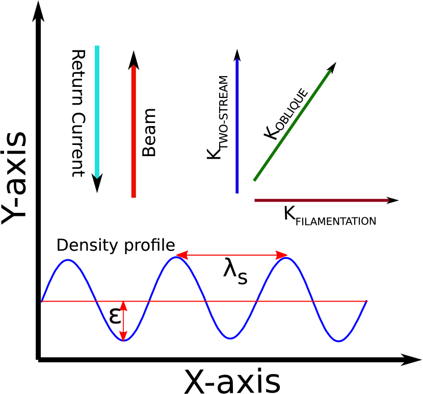
Figure 1: Sketch of the system considered in the present article.

We employ a two fluid description wherein the relativistic electron beam (REB) and the background electrons are treated as separate fluids. The evolution equations of these two electron species are coupled with the Maxwell’s equations which governs the field evolution. The ions are assumed to be static and merely provide a neutralizing background. A collision-less, quasi-neutral and un-magnetized electron beam-plasma system is considered. The electron beam drift in the ŷ direction inducing a return current in cold background plasma electrons ($T_{0p}$). The initial configuration is chosen so as to have charge and current neutrality. The sketch of the configuration is shown in Fig. 1. At time t=0, a space dependent (transverse to the beam flow direction) background ion density $n_{0i}$ is chosen. The charge neutrality condition is fulfilled by choosing the sum of the beam density $n_{0b}$ and the background electron density $n_{0p}$ to match with background density of ions. The system can be described by following set of dimensionless governing equations:

$$\frac{\partial n_{\alpha}}{\partial t}+\nabla\cdot\left(n_{\alpha}\vec{v_{\alpha}}\right)=0$$ (1)

$$\frac{\partial\vec{p_{\alpha}}}{\partial t}+\vec{v_{\alpha}}\cdot\nabla\vec{p_{\alpha}}=-\left(\vec{E}+\vec{v_{\alpha}}\times\vec{B}\right)-\frac{\nabla P_{\alpha}}{n_{\alpha}}$$ (2)

$$\frac{\partial\vec{B}}{\partial t}=-\nabla\times\vec{E}$$ (3)

$$\frac{\partial\vec{E}}{\partial t}=\nabla\times\vec{B}-\Sigma_{\alpha}{\vec{J_{\alpha}}}$$ (4)

with $\vec{v}_{\alpha}={\vec{p_{\alpha}}}/{(1+{p_{\alpha}}^{2})^{\frac{1}{2}}}$ where $\vec{p_{\alpha}}$ is momentum vector, $\vec{J_{\alpha}}=-n_{\alpha}\vec{v_{\alpha}}$. The pressure $P_{\alpha}$ is provided by the equation of state. In the above equations, velocity is normalized by the speed of light $c$, density by $n_{0}$ (the spatially average ion density), frequency by $\omega_{0}=\sqrt{4\pi n_{0}^{2}e/m_{e}}$, length by electron skin depth $d_{e}=c/\omega_{0}e$ and electric and magnetic field by $E_{0}=B_{0}=m_{e}c\omega_{0}/e$ where $m_{e}$ is electron rest mass and $e$ is electron charge. The subscript $\alpha$ is ${}^{\prime}b^{\prime}$ for beam and ${}^{\prime}p^{\prime}$ for plasma.

In the equilibrium there is no electric and magnetic field, so there is complete charge as well as current neutralization. This is achieved by balancing the forward and return electron currents at each spatial location. For simplicity of treatment, the profile of transverse temperature $T_{\alpha}$ is chosen in such a way that gradient of pressure is zero in equilibrium. The temperature parallel to beam propagation direction has been chosen to be negligible. The background plasma is chosen to be cold ($T_{0p}=0$) in all our analytical as well simulation studies. Thus, for an inhomogeneous case considered by us in this work we have the following conditions for equilibrium:

$$n_{0i}(x)=n_{0b}(x)+n_{0p}(x)$$ (5)

$$\Sigma_{\alpha}n_{0\alpha}(x)\vec{v_{0\alpha}}=0$$ (6)

In equilibrium beam pressure $P_{0b}$ is chosen to be independent of x. This is achieved by choosing the beam temperature $T_{0b}(x)$ to be satisfying the following condition

$$P_{0b}=T_{0b}(x)n_{0b}(x)=constant=C.$$ (7)

$$T_{0b}(x)=C/n_{0b}(x)$$ (8)

The suffix $0$ indicates the equilibrium fields. We linearize equations (1)-(4) to obtain linear growth rate of the instability. The inhomogeneity being periodic along ${}^{\prime}x^{\prime}$ we choose all the perturbed quantities to have the form of $f_{\alpha}=\Sigma_{j}^{....,\pm 2,\pm 1,0}f_{\alpha j}e^{i((k_{x}+jk_{s})x+k_{y}y-\omega t)}$. Here $k_{s}$ is the wavenumber associated with the periodic profile of inhomogeneity. For small amplitude of inhomogeneity$(\varepsilon<1)$, the terms corresponding to $j=0,\pm 1$ are the ones which are only retained. All higher order terms are neglected. The coupled set of differential equations obtained after linearizing Eqs.(1)-(4) are following :

$$\Omega_{\alpha}\gamma_{0\alpha}^{3}v_{l\alpha y}^{\prime\prime}+\left(\omega^{2}-k_{y}^{2}\right)\Omega_{\alpha}\gamma_{0\alpha}^{3}v_{l\alpha y}+\left(\omega^{2}-k_{y}^{2}\right)\sum_{\alpha}\frac{n_{0\alpha}}{\Omega_{\alpha}}v_{l\alpha y}+\sum_{\alpha}\frac{k_{y}-\omega v_{0\alpha}}{\Omega_{\alpha}}\left(n_{0\alpha}v_{l\alpha y}\right)^{\prime}=0$$ (9)

$$\hskip 22.76228pt\frac{(\omega^{2}-k_{y}^{2})}{\Omega_{\alpha}}\eta T_{0\alpha}v_{l\alpha x}^{\prime\prime}-\frac{(\omega^{2}-k_{y}^{2})}{\Omega_{\alpha}}\eta T_{0\alpha}^{\prime}v_{l\alpha x}^{\prime}+\left(\frac{(\omega^{2}-k_{y}^{2})}{n_{0\alpha}\Omega_{\alpha}}\eta T_{0\alpha}^{\prime}n_{0\alpha}^{\prime\prime}+(\omega^{2}-k_{y}^{2})\Omega_{\alpha}\gamma_{0\alpha}\right)v_{l\alpha x}$$ (10)

$$\hskip 22.76228pt-\Omega_{\alpha}\sum_{\alpha}n_{0\alpha}v_{l\alpha x}+\left(i\frac{k_{y}}{\Omega_{\alpha}}(\omega^{2}-k_{y}^{2})\eta T_{0\alpha}-i\left(k_{y}-v_{0\alpha}\omega\right)\Omega_{\alpha}\gamma^{3}_{0\alpha}\right)v_{l\alpha y}^{\prime}=0$$

Where $\Omega_{\alpha}$=$(\omega-k_{y}v_{0}\alpha)$ and $\eta$ is ratio of specific heat. When the plasma density is homogeneous i.e. $\varepsilon=0$, these coupled equations reduce to the standard linear equations for the beam plasma system:

$$\Omega_{\alpha}\gamma_{0\alpha}^{3}v_{l\alpha y}^{\prime\prime}+\left(\omega^{2}-k_{y}^{2}\right)\Omega_{\alpha}\gamma_{0\alpha}^{3}v_{l\alpha y}+\left(\omega^{2}-k_{y}^{2}\right)\sum_{\alpha}\frac{n_{0\alpha}}{\Omega_{\alpha}}v_{l\alpha y}+\sum_{\alpha}\frac{k_{y}-\omega v_{0\alpha}}{\Omega_{\alpha}}n_{0\alpha}v_{l\alpha y}^{\prime}=0$$ (11)

$$\frac{(\omega^{2}-k_{y}^{2})}{\Omega_{\alpha}}\eta T_{0\alpha}v_{l\alpha x}^{\prime\prime}+\left(\omega^{2}-k_{y}^{2}\right)\Omega_{\alpha}\gamma_{0\alpha}v_{l\alpha x}-\Omega_{\alpha}\sum_{\alpha}n_{0\alpha}v_{l\alpha x}$$

$$\hskip 153.6447pt+\left(i\frac{k_{y}}{\Omega_{\alpha}}(\omega^{2}-k_{y}^{2})\eta T_{0\alpha}-i\left(k_{y}-v_{0\alpha}\omega\right)\Omega_{\alpha}\gamma^{3}_{0\alpha}\right)v_{l\alpha y}^{\prime}=0$$ (12)

In the next section we study in detail the growth rate of the most unstable mode for the general case by using eq. (10).

III Analytical Study

The linear evolution of beam-plasma system is studied by choosing sinusoidal form of ion background density of the form $n_{0i}=n_{0}(1+\varepsilon cos(k_{s}x))$ where $n_{0}$ is constant normalized density, $\varepsilon$ is inhomogeneity amplitude and $k_{s}=2\pi m/L_{x}$ ($m$ is an integer and $L_{x}$ is the system dimension along $x$) is inhomogeneity wave vector. The equilibrium beam and plasma density profile have been taken as $n_{0b}=\beta_{b}n_{0}(1+\varepsilon_{b}cos(k_{s}x))$, $n_{0p}=\beta_{p}n_{0}(1+\varepsilon_{p}cos(k_{s}x))$ to maintain quasi neutrality where $\sum_{\alpha}\beta_{\alpha}=1$ is a fraction. For simplicity, we have chosen $\varepsilon_{b}=\varepsilon_{p}=\varepsilon$ here.

To evaluate the linear growth rate of oblique mode driven instability, we expand eq. (10) and eq. (LABEL:vx_in) and solve it by substituting for the Bloch wave function form of the perturbed fields in the periodic system. Retaining only the first order terms, as mentioned earlier we obtain:

$$\Omega_{\alpha}\gamma_{0\alpha}^{3}\left(\lambda^{2}-k_{d}^{2}\right)v_{d\alpha y}+\lambda^{2}\sum_{\alpha}\frac{\beta_{\alpha}}{\Omega_{\alpha}}v_{d\alpha y}+\lambda^{2}\sum_{\alpha}\frac{0.5\varepsilon\beta_{\alpha}}{\Omega_{\alpha}}v_{\alpha y}+i\sum_{\alpha}\frac{\zeta_{\alpha}}{\Omega_{\alpha}}\beta_{\alpha}k_{d}v_{d\alpha x}$$

$$\hskip 290.21802pt+i\sum_{\alpha}\frac{\zeta_{\alpha}}{\Omega_{\alpha}}0.5\varepsilon\beta_{\alpha}k_{d}v_{\alpha x}=0$$

$$\Omega_{\alpha}\gamma_{0\alpha}^{3}\left(\lambda^{2}-k_{o}^{2}\right)v_{\alpha y}+\lambda^{2}\sum_{\alpha}\frac{\beta_{\alpha}}{\Omega_{\alpha}}v_{\alpha y}+\lambda^{2}\sum_{\alpha}\frac{0.5\varepsilon\beta_{\alpha}}{\Omega_{\alpha}}\left(v_{d\alpha y}+v_{a\alpha y}\right)+i\sum_{\alpha}\frac{\zeta_{\alpha}}{\Omega_{\alpha}}\beta_{\alpha}k_{o}v_{\alpha x}$$

$$\hskip 227.62204pt+i\sum_{\alpha}\frac{\zeta_{\alpha}}{\Omega_{\alpha}}0.5\varepsilon\beta_{\alpha}k_{o}\left(v_{d\alpha x}+v_{a\alpha x}\right)=0$$

$$\Omega_{\alpha}\gamma_{0\alpha}^{3}\left(\lambda^{2}-k_{a}^{2}\right)v_{a\alpha y}+\lambda^{2}\sum_{\alpha}\frac{\beta_{\alpha}}{\Omega_{\alpha}}v_{a\alpha y}+\lambda^{2}\sum_{\alpha}\frac{0.5\varepsilon\beta_{\alpha}}{\Omega_{\alpha}}v_{\alpha y}+i\sum_{\alpha}\frac{\zeta_{\alpha}}{\Omega_{\alpha}}\beta_{\alpha}k_{a}v_{a\alpha x}$$

$$\hskip 290.21802pt+i\sum_{\alpha}\frac{\zeta_{\alpha}}{\Omega_{\alpha}}0.5\varepsilon\beta_{\alpha}k_{a}v_{\alpha x}=0$$

$$\left(\frac{\lambda^{2}}{\Omega_{\alpha}\beta_{\alpha}}\eta c_{\alpha}k_{d}^{2}-\lambda^{2}\Omega_{\alpha}\gamma_{0\alpha}\right)v_{d\alpha x}+\Omega_{\alpha}\sum_{\alpha}\beta_{\alpha}v_{d\alpha x}+0.5\varepsilon\frac{\lambda^{2}}{\Omega_{\alpha}\beta_{\alpha}}\eta c_{\alpha}[k_{d}^{2}-k_{0}(2k_{0}-k_{s})]v_{\alpha x}$$

$$+0.5\varepsilon\Omega_{\alpha}\sum_{\alpha}\beta_{\alpha}v_{\alpha x}+\left(k_{y}k_{d}\frac{\lambda^{2}}{\Omega_{\alpha}\beta_{\alpha}}\eta c_{\alpha}-\zeta_{\alpha}\Omega_{\alpha}\gamma_{0\alpha}^{3}k_{d}\right)v_{d\alpha y}-0.5\varepsilon\frac{\lambda^{2}}{\Omega_{\alpha}\beta_{\alpha}}\eta c_{\alpha}k_{y}k_{0}v_{\alpha y}=0$$

$$\left(\frac{\lambda^{2}}{\Omega_{\alpha}\beta_{\alpha}}\eta c_{\alpha}k_{0}^{2}-\lambda^{2}\Omega_{\alpha}\gamma_{0\alpha}\right)v_{\alpha x}+\Omega_{\alpha}\sum_{\alpha}\beta_{\alpha}v_{\alpha x}+0.5\varepsilon\frac{\lambda^{2}}{\Omega_{\alpha}\beta_{\alpha}}\eta c_{\alpha}[k_{0}^{2}-k_{d}(2k_{d}+k_{s})]v_{d\alpha x}+$$

$$0.5\varepsilon\frac{\lambda^{2}}{\Omega_{\alpha}\beta_{\alpha}}\eta c_{\alpha}[k_{0}^{2}-k_{a}(2k_{a}-k_{s})]v_{a\alpha x}+0.5\varepsilon\Omega_{\alpha}\sum_{\alpha}\beta_{\alpha}\left(v_{d\alpha x}+v_{a\alpha x}\right)$$

$$+ \left(k_{y}k_{0}\frac{\lambda^{2}}{\Omega_{\alpha}\beta_{\alpha}}\eta c_{\alpha}-\zeta_{\alpha}\Omega_{\alpha}\gamma_{0\alpha}^{3}k_{0}\right)v_{\alpha y}-0.5\varepsilon\frac{\lambda^{2}}{\Omega_{\alpha}\beta_{\alpha}}\eta c_{\alpha}k_{y}\left(k_{d}v_{d\alpha y}+k_{a}v_{a\alpha y}\right)=0$$ (18)

$$\left(\frac{\lambda^{2}}{\Omega_{\alpha}\beta_{\alpha}}\eta c_{\alpha}k_{a}^{2}-\lambda^{2}\Omega_{\alpha}\gamma_{0\alpha}\right)v_{a\alpha x}+\Omega_{\alpha}\sum_{\alpha}\beta_{\alpha}v_{a\alpha x}+0.5\varepsilon\frac{\lambda^{2}}{\Omega_{\alpha}\beta_{\alpha}}\eta c_{\alpha}[k_{a}^{2}-k_{0}(2k_{0}+k_{s})]v_{\alpha x}$$

$$+0.5\varepsilon\Omega_{\alpha}\sum_{\alpha}\beta_{\alpha}v_{\alpha x}+\left(k_{y}k_{d}\frac{\lambda^{2}}{\Omega_{\alpha}\beta_{\alpha}}\eta c_{\alpha}-\zeta_{\alpha}\Omega_{\alpha}\gamma_{0\alpha}^{3}k_{a}\right)v_{a\alpha y}-0.5\varepsilon\frac{\lambda^{2}}{\Omega_{\alpha}\beta_{\alpha}}\eta c_{\alpha}k_{y}k_{0}v_{\alpha y}=0$$

where $\lambda^{2}=\left(\omega^{2}-k_{y}^{2}\right)$, $k_{d}=(k_{x}-k_{s})$, $k_{0}=k_{x}$, $k_{a}=(k_{x}+k_{s})$ and $\zeta_{=}(k_{y}-v_{0\alpha}\omega)$.

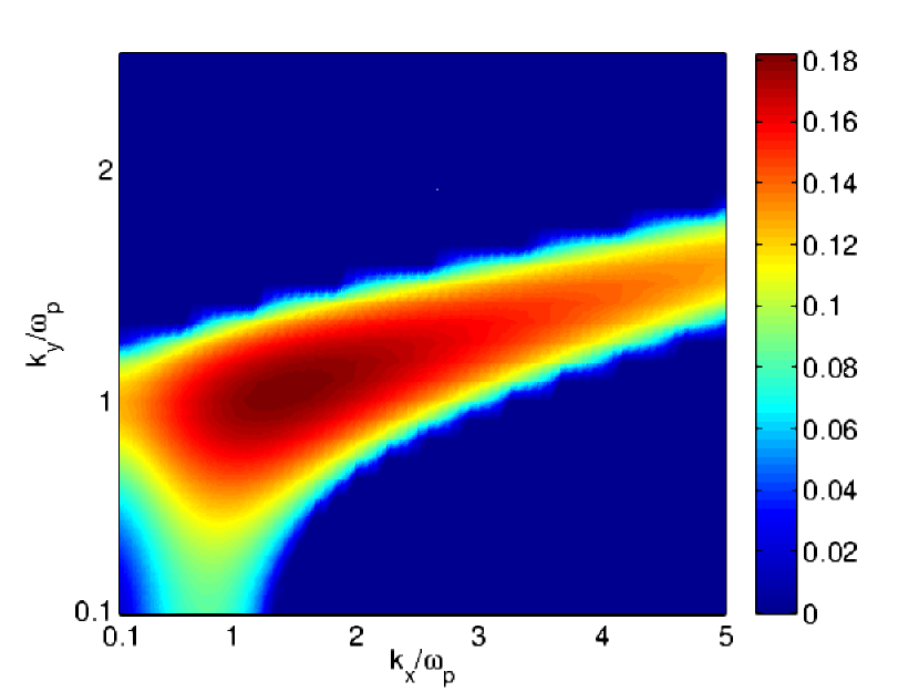
Figure 2: Growth rate map of the 2D oblique instability for a homogeneous beam-plasma at transverse beam temperature $T_{b0\perp}$=10 keV.

The map of the growth rate in the parameter space of $k_{x}$ and $k_{y}$ for the homogeneous system has been shown in Fig. 2 for $n_{0b}/n_{0p}=1/9$ or $n_{0b}/n_{0e}=0.1$, $v_{0b}=0.9c$, $v_{0p}=-0.1c$ and $T_{0b\perp}=10KeV$. This map shows that for this particular set of parameters, oblique mode with($k_{x}$, $k_{y}$=(1.5,1)) has a maximum growth rate. Also a narrow oblique strip of wavenumbers extending up to $k_{x}$ =$\infty$ is found to be unstable.

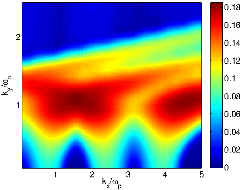
Figure 3: Growth rate map of the 2D oblique instability for a inhomogeneous beam-plasma at transverse beam temperature $T_{b0\perp}$=10 keV at $k_{s}=\pi$ and $\varepsilon=0.1$.

When the plasma density in chosen to be inhomogeneous and the scale length of the inhomogeneity is longer than the skin depth, i.e. $2\pi/k_{s}>c/\omega_{0}$ the growth rate of oblique mode driven instability is observed to increase with the inhomogeneity amplitude $\varepsilon$, as shown in Fig. 3 and  4. The unstable modes continues to stay around the oblique patch in the $k_{x}$ vs. $k_{y}$ plane. However, the growth rate is spread over a wider $k_{y}$ domain compared to the homogeneous case. Another feature is the appearance of several maxima along $k_{x}$ in contrast to the single extrema for the homogeneous case.

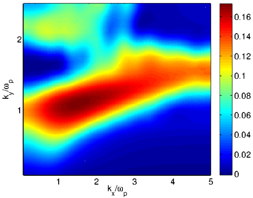
Figure 5: Growth rate map of the 2D oblique mode driven instability for a inhomogeneous beam-plasma at transverse beam temperature $T_{b0\perp}$=10 keV at $k_{s}=3\pi$ and $\varepsilon=0.1$.

When the inhomogeneity scale length is sharper than the skin depth, i.e. for the case of $2\pi/k_{s}\leq c/\omega_{0}$, there is an overall reduction of the growth rates in the system in comparison to the homogeneous case. Furthermore, with increasing amplitude of density inhomogeneity also the growth rate reduces in this regime. This has been illustrated in the 2-D plot of the growth rate in Fig. 5 and  6.

A detailed comparison of the growth rate $\Gamma_{gr}$ of the maximally growing mode for various different values of $k_{s}$ and $\varepsilon$ has been provided in TABLE I.

TABLE I

The maximum growth rate of oblique mode driven instability evaluated analytically under the approximation of weak inhomogeneity amplitude as well as from PIC simulation. $\varepsilon$ $k_{s}$ $\Gamma_{gr}$(max.) $\Gamma_{pic}$(max.) 0.0 0.0 0.1822 0.1823 0.1 $\pi$ 0.1857 0.1827 0.1 $2\pi$ 0.1811 0.1818 0.1 $3\pi$ 0.1728 0.1813 0.2 $\pi$ 0.1884 0.1830 0.2 $3\pi$ 0.1475 0.1659 0.4 $3\pi$ 0.1352 0.16

It is clear from the results that the growth rate drops when the amplitude as well as the wave number of the plasma density inhomogeneity is increased.

IV PIC Simulation

In this section, we present the results from the $2\frac{1}{2}$D PIC simulations employed for the study of beam plasma instabilities for an inhomogeneous density plasma. The simulation box is a Cartesian $X\times Y$ plane with periodic boundary condition for both the electromagnetic field and charged particles. The initial choice of configuration satisfies the equilibrium condition. The electron beam is chosen to propagate in the $\hat{y}$ direction with a relativistic velocity $v_{0b}$ whose current is neutralized by the cold return shielding current from the background plasma electron flowing in the opposite direction with a velocity $v_{0p}$. The respective densities are appropriately chosen for the current to be zero. Charge neutrality and a null current density are both ensured initially ($t=0$). Thus, the system is field free and in equilibrium initially.

The electron beam has also been chosen to have a finite temperature $T_{0b}$. For the inhomogeneous plasma the pressure contribution in such cases have been avoided by choosing $T_{0b}$ to be space dependent defined by eq. 8. The ions are kept at rest during the simulation. The uniform plasma density $n_{0e}$ is taken as $10n_{c}$ where $n_{c}=1.1\times 10^{21}cm^{-3}$ is the critical density for 1$\mu$m wavelength of laser light. The area of the simulation box R is $30\times 15$ $(c/\omega_{0})^{2}$ corresponding to $1500\times 750$ cells where $c/\omega_{0}=d_{e}=5.0\times 10^{-2}\mu$m is the skin depth. The total number of particles is $45000000$ each for both electrons and ions. To resolve the underlying physics at the scale which is smaller than the skin depth, we have chosen a grid size of 0.02$d_{e}$. The time step is decided by the Courant condition. The time evolution of the box averaged field energy density for every component of $\vec{E}$ and $\vec{B}$ are recorded at each time step. The energy density is normalized with respect to $(m_{e}c\omega_{0}/e)^{2}$ and time is normalized with respect to the electron plasma frequency $\omega_{0}$. The results obtained from the simulation of the beam-plasma system for various amplitudes and scale lengths of inhomogeneity have been compared with the results of the homogeneous beam-plasma case. The initial choices of the parameters for simulation are taken as $n_{0b}/n_{0p}=1/9$ or $n_{0b}/n_{0e}=0.1$, $v_{0b}=0.9c$, $v_{0p}=-0.1c$ and $T_{0b\perp}=10KeV$. These parameters favor the growth of the oblique mode over the filamentation and two-stream modes. While considering the simulation of the inhomogeneous case, the inhomogeneity amplitudes $\varepsilon$ is varied from $0.1$ to $0.2$. The inhomogeneity wavenumber is chosen as $k_{s}$=$\pi$, $2\pi$ and $3\pi$ for each of these amplitudes.

The perturbed field energies (magnetic as well as electric) are tracked in the simulation for the study of instabilities associated with the system. The rate of exponential growth of the perturbed energy provides for twice the growth rate of the fastest growing mode associated with the instability. The growth rates $\Gamma_{pic}$(max.), thus evaluated for different cases of simulations have been presented in one column of TABLE I.

The linear regime can be clearly identified from a log plot of total energy shown in (Fig. 7). The region of constant slope after an initial transient provides the growth rate of the fastest growing mode. The straight line alongside represents the slope obtained from the linear theory provided in section II. It can be observed that the agreement between simulation and the theoretical linear results are remarkably good. The comparison also shows that the reduction in the growth rate in the presence of inhomogeneity in plasma density for scales sharper than the skin depth.

The separate evolution of electric field energy density and the magnetic field energy density for various simulation cases have been shown in Fig. 8 and Fig. 9 respectively. The energy associated with electric field is observed to be typically always higher than the energy in magnetic field. It is interesting to compare these perturbed energies in the nonlinear regime. While for the homogeneous case the energy continues to remain high, there is a perceptible drop in both electric and magnetic field the energies in the presence of inhomogeneity in the nonlinear regime. This has important significance as it suggests that the forward and reverse currents which got separated during the linear phase have a tendency to merge again for the inhomogeneous density when nonlinearity sets in the system.

The snapshot of the spatial profile in the $x-y$ plane of certain fields ($B_{s}$, $n_{b}$ and $n_{p}$) at a time $\omega_{0}t=$33, 53 and 90 have been shown in Figs. 10, 11 and 12 respectively. In these figures the first column corresponds to the homogeneous case, i.e. $\varepsilon=0.0$ and second column to the inhomogeneous case with $\varepsilon=0.2$ and $k_{s}=3\pi$ (corresponding to density inhomogeneity scale lengths to be sharper than the skin depth). It is clear from these figures that the variations in these fields are in both ${}^{\prime}x^{\prime}$ as well as ${}^{\prime}y^{\prime}$ directions, confirming that the oblique mode continues to dominate the instability scene. However, it should also be noted that during the linear phase the magnetic field acquires structures which are extended and aligned along the beam flow direction of $\hat{y}$. The structure size along the $x$ direction is significantly shorter and is found to compare with the typical values of the skin depth. In the inhomogeneous case additional structures at the shorter inhomogeneity scale are observed to ride over those appearing at the skin depth scale. As an aside we wish to mention that fluid simulations based on Electron Magnetohydrodynamic model has also shown that plasma density inhomogeneity leads to the guiding of electron current structures sharad . These studies, therefore, suggest that specially tailored targets incorporating appropriate forms of plasma density inhomogeneity can in fact be helpful for efficient transport of electron beam through plasmas.

V Summary

In this work instability of the beam plasma system has been analyzed for the case when the background plasma is chosen to be inhomogeneous. The linear analytical evaluation of growth rate shows that when the inhomogeneity scale length is shorter than the typical skin depth scale of the plasma the growth rate of the instability is suppressed. A quantitative comparison of the growth rate of the maximally growing mode for the homogeneous and inhomogeneous cases were made, which clearly show the reduction in the growth rate in the presence of density inhomogeneity with sharper scales. A detailed PIC simulation in 2-D have also been performed which confirms this. The simulation shows reduced growth rate and also the channelizing of current during the linear phase.

Our work has direct relevance to the recent experimental work on the observation of efficient transport of Mega Ampere of electron currents through aligned carbon nanotube arrays. The ionization of the carbon nanotubes by the prepulse of laser pulse would produce an inhomogeneous plasma density. The suppression of the beam plasma instabilities would then aid the process of efficient transport of electron current as observed in the experiment.

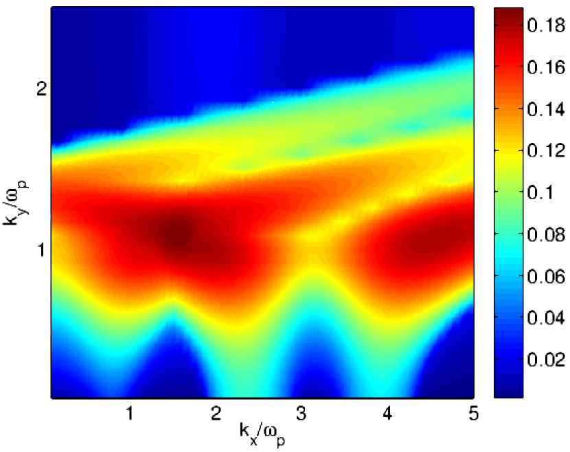
Figure 4: Growth rate map of the 2D oblique mode driven instability for a inhomogeneous beam-plasma at transverse beam temperature $T_{b0\perp}$=10 keV at $k_{s}=\pi$ and $\varepsilon=0.2$.

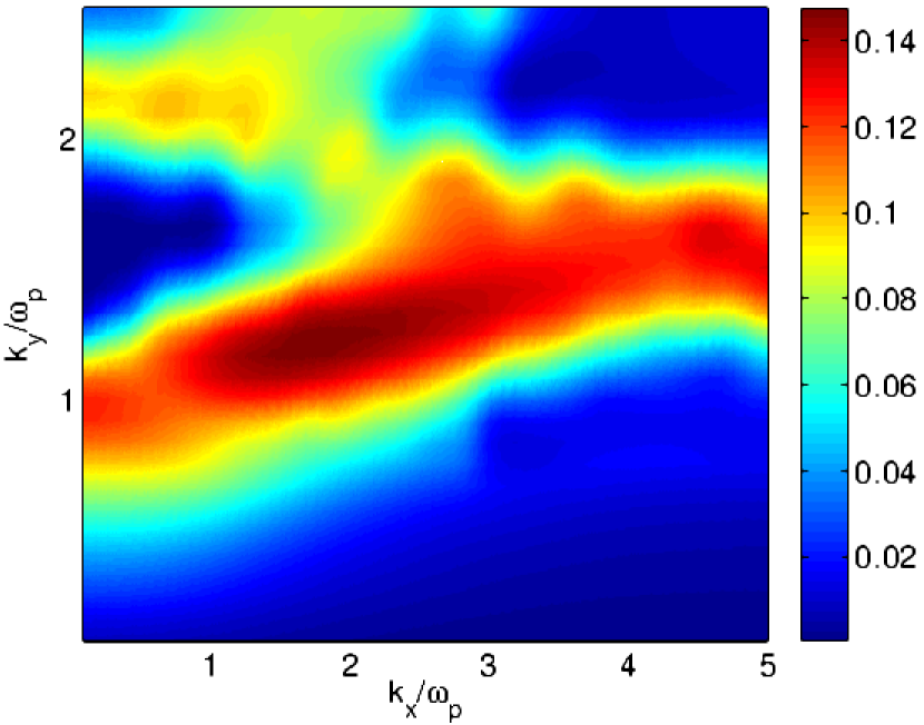
Figure 6: Growth rate map of the 2D oblique mode driven instability for a inhomogeneous beam-plasma at transverse beam temperature $T_{b0\perp}$=10 keV at $k_{s}=3\pi$ and $\varepsilon=0.2$.

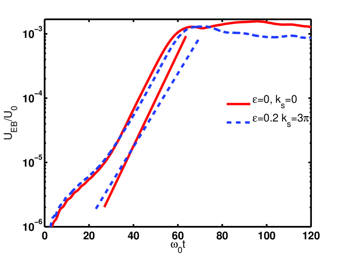
Figure 7: Growth rate from PIC simulation by energy slope.

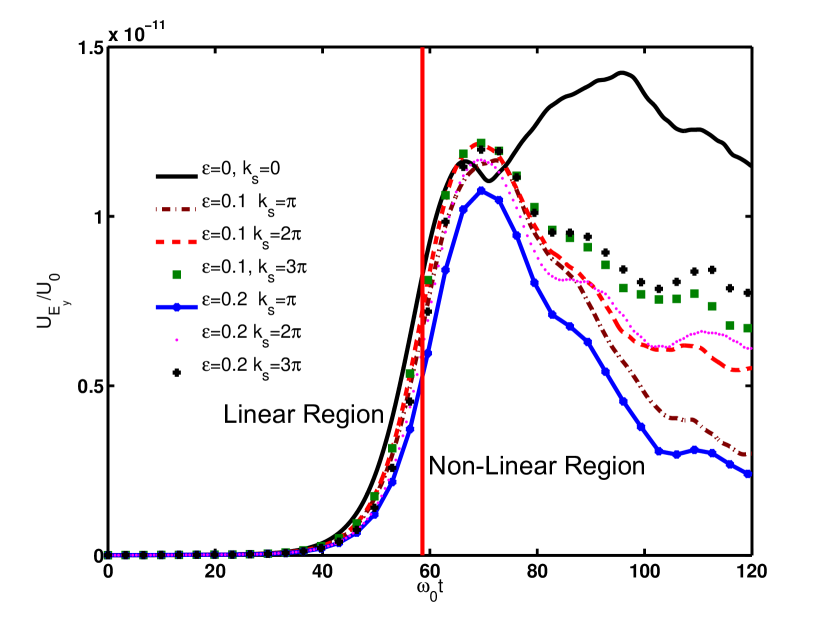
Figure 8: The evolution of y-component of normalized electric field energies $U_{E_{y}}$ with time for homogeneous and inhomogeneity cases.

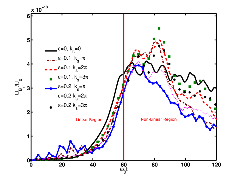
Figure 9: The evolution of z-component of normalized magnetic field energies $U_{B_{z}}$ with time for homogeneous and inhomogeneity cases.

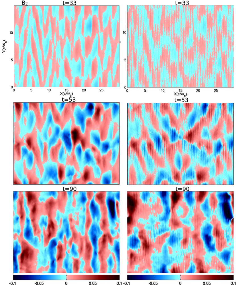
Figure 10: Time evolution and spatial configuration of z-component of magnetic field for homogeneous (first column) and inhomogeneous ($\varepsilon$=0.2 at $k_{s}$=$3\pi$, last column) case at time $\omega_{0}t=33$, $\omega_{0}t=53$ and $\omega_{0}t=90$.

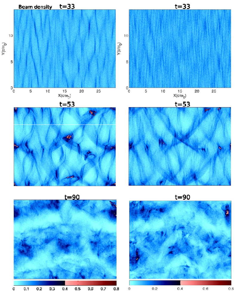
Figure 11: Time evolution and spatial configuration of beam density for homogeneous (first column)and inhomogeneous ($\varepsilon$=0.2 at $k_{s}$=$3\pi$, last column) case at time $\omega_{0}t=33$, $\omega_{0}t=53$ and $\omega_{0}t=90$.

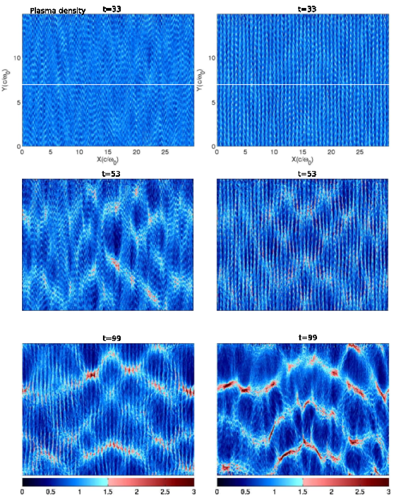
Figure 12: Time evolution and spatial configuration of background electron plasma density for homogeneous (first column)and inhomogeneous ($\varepsilon$=0.2 at $k_{s}$=$3\pi$, last column) case at time $\omega_{0}t=33$, $\omega_{0}t=53$ and $\omega_{0}t=90$.

References

- [1] M. Tabak, D. S. Clark, S. P. Hatchett, M. H. Key, B. F. Lasinski, R. A. Snavely, S. C. Wilks, R. P. J. Town, R. Stephens, E. M. Campbell, R. Kodama, K. Mima, K. A. Tanaka, S. Atzeni, and R. Freeman. Physics of Plasmas, 12, 057305 (2005).
- [2] G. Malka and J. L. Miquel. Phys. Rev. Lett. 77, 75 (1996).
- [3] Marian Karlický. The Astrophysical Journal 690, 189 (2009).
- [4] M. Lazar, R. Schlickeiser, R. Wielebinski, and S. Poedts. The Astrophysical Journal 693, 1133 (2009).
- [5] F. Califano, N. Attico, F. Pegoraro, G. Bertin, and S. V. Bulanov. Phys. Rev. Lett. 86, 5293 (2001).
- [6] A. Modena. Nature 377, 606 (1995).
- [7] K. B. Wharton, S. P. Hatchett, S. C. Wilks, M. H. Key, J. D. Moody, V. Yanovsky, A. A. Offenberger, B. A. Hammel, M. D. Perry, and C. Joshi. Phys. Rev. Lett. 81, 822 (1998).
- [8] D. Bohm and E. P. Gross. Phys. Rev. 75, 1851 (1949).
- [9] Burton D. Fried. Physics of Fluids 2, 337 (1959).
- [10] Roswell Lee and Martin Lampe. Phys. Rev. Lett. 31, 1390 (1973).
- [11] Erich S. Weibel. Phys. Rev. Lett. 2, 83 (1959).
- [12] T. Taguchi, T. M. Antonsen, and K. Mima. Computer Physics Communications, 164, 269 (2004).
- [13] A. Bret, M.-C. Firpo, and C. Deutsch. Phys. Rev. E, 70, 046401 (2004).
- [14] Jacob Trier Frederiksen and Mark Eric Dieckmann. Physics of Plasmas, 15, 094503 (2008).
- [15] M. E. Dieckmann, J. T. Frederiksen, A. Bret, and P. K. Shukla. Physics of Plasmas, 13, 112110 (2006).
- [16] A. Bret and C. Deutsch. Physics of Plasmas, 12, 082704 (2005).
- [17] A. Bret, L. Gremillet, and M. E. Dieckmann. Physics of Plasmas, 17, 120501 (2010).
- [18] A. R. Bell and R. J. Kingham. Phys. Rev. Lett. 91, 035003 (2003).
- [19] B. Ramakrishna, S. Kar, A. P. L. Robinson, D. J. Adams, K. Markey, M. N. Quinn, X. H. Yuan, P. McKenna, K. L. Lancaster, J. S. Green, R. H. H. Scott, P. A. Norreys, J. Schreiber, and M. Zepf. Phys. Rev. Lett. 105, 135001 (2010).
- [20] Gourab Chatterjee, Prashant Kumar Singh, Saima Ahmed, A. P. L. Robinson, Amit D. Lad, Sudipta Mondal, V. Narayanan, Iti Srivastava, Nikhil Koratkar, John Pasley, A. K. Sood, and G. Ravindra Kumar. Phys. Rev. Lett. 108, 235005 (2012).
- [21] S. K. Mishra, Predhiman Kaw, A. Das, S. Sengupta, and G. Ravindra Kumar. Physics of Plasmas , 21, 012108 (2014).
- [22] Chandrasekhar Shukla, Amita Das and Kartik Patel. Phys. Scr. 90, 0856052015 (2015).
- [23] Sharad Kumar Yadav, Amita Das and Predhiman Kaw. Physics of Plasmas , 15, 062308 (2008).