Top Mode pseudo Nambu-Goldstone Boson Higgs Model

Abstract

We discuss the Top Mode pseudo Nambu-Goldstone boson Higgs (TMpNGBH) model which has recently been proposed as a variant of the top quark condensate model in light of the 125 GeV Higgs boson discovered at the LHC. In this talk, we focus on the vacuum alignment and the phenomenologies of characteristic particles of the TMpNGBH model.

1 Introduction

The ATLAS [4] and CMS collaborations [5] have discovered a $125\,\text{GeV}$ Standard Model (SM)-like Higgs boson. This implies that the era to reveal the origin of mass of the elementary particles has come. Preceding the discovery of the Higgs boson by about two decades the top quark has been discovered at the Tevatron [6, 7]. The top quark is the heaviest particle among the observed particles and its mass is $m_{t}\simeq 173\,\text{GeV}$ [8], which is coincidentally on the order of the Higgs mass and the electroweak symmetry breaking (EWSB) scale ($v_{{}_{\rm EW}}\simeq 246\,\text{GeV}$).

The top quark condensate model [9, 10, 11] is a scenario in which the top quark plays a crucial role to explain the dynamical origin for both the EWSB and the Higgs boson. However, the original top quark condensate model is somewhat far from a realistic situation, especially, a Higgs boson predicted as a $t\bar{t}$ bound state has the mass in a range of $m_{t}\hskip 3.00003pt\raisebox{1.72218pt}{$<$}\raisebox{-3.01385pt}{$\sim$}\hskip 3.00003ptm_{H}\hskip 3.00003pt\raisebox{1.72218pt}{$<$}\raisebox{-3.01385pt}{$\sim$}\hskip 3.00003pt2m_{t}$, which cannot be identified with the $125\,\text{GeV}$ Higgs boson at the LHC.

2 Top-Mode pseudo Nambu-Goldstone Boson Higgs (TMpNGBH) model

Recently, a variant class of the top quark condensate model, so-called Top-Mode pseudo Nambu-Goldstone Boson Higgs (TMpNGBH) model, was proposed [1, 12]. In these models a composite Higgs boson emerges as a pseudo Nambu–Goldstone boson (pNGB) associated with the spontaneous breaking of a global symmetry, therefore it is light to be identified as the LHC Higgs boson.

The TMpNGBH model is constructed from the top and bottom quarks $q=(t,b)$ and a vectorlike $\chi$ quark, a flavor partner of the top quark having the same SM charges as those of the right-handed top quark, which form a four-fermion interaction:

$${\cal L}_{4f}=G_{4f}(\bar{\psi}^{i}_{L}\chi_{R})(\bar{\chi}_{R}\psi^{i}_{L})\,,$$ (1)

where $\psi^{i}_{L}\equiv(t_{L},b_{L},\chi_{L})^{T\,i}\,\,(i=1,2,3)$. This four-fermion interaction possesses the global symmetry $G=U(3)_{L}\times U(1)_{R}$. When the value of $G_{4f}$ is large enough to form a fermion-bilinear condensate, namely $G_{4f}>G_{\rm crit}=8\pi^{2}/(N_{c}\Lambda^{2})$ with $N_{c}$ being the number of QCD color and $\Lambda$ the cutoff scale of the theory, the global symmetry is spontaneously broken down to $H=U(2)_{L}\times U(1)_{V}$. In association with the symmetry breaking, the five NGBs emerge as bound states of the $t$ and $\chi$ quarks, in addition to a composite heavy scalar boson, corresponding to the $\sigma$ mode of the usual Nambu-Jona-Lasinio (NJL) model [13]. Three of these five NGBs are eaten by the electroweak gauge bosons when the subgroup of $G$ is gauged by the electroweak symmetry (and if the condensate is formed in a direction where the electroweak symmetry is broken). The other two remain as physical states, and they obtain their masses by additional interaction terms which explicitly break the global $G=U(3)_{L}\times U(1)_{R}$ symmetry:

$${\cal L}_{h}=-\left[\Delta_{\chi\chi}\bar{\chi}_{R}\chi_{L}+\text{h.c.}\right]-G^{\prime}\left(\bar{\chi}_{L}\chi_{R}\right)\left(\bar{\chi}_{R}\chi_{L}\right)\,.$$ (2)

Then two NGBs become pNGBs, dubbed as top-mode pNGBs (TMpNGBs). One of the TMpNGBs, which is the $CP$-even scalar ($h^{0}_{t}$), is identified as the $126\,\text{GeV}$ Higgs boson discovered at the LHC, while the other is the $CP$-odd scalar ($A^{0}_{t}$). Furthermore, the model includes another four-fermion interaction term,

$${\cal L}_{t}=G^{\prime\prime}\left(\bar{\chi}_{L}\chi_{R}\right)\left(\bar{t}_{R}\chi_{L}\right)+\text{h.c.}\,.$$ (3)

This, combined with Eq.(1), generates the top quark mass via the top-seesaw mechanism [14, 15, 16, 17, 18].

Note that Eq.(3) also explicitly breaks the $G$-symmetry, but does not contribute to the TMpNGBs’ masses ($m_{h^{0}_{t}}$ and $m_{A^{0}_{t}}$) at the leading order. However, it was shown that at the next-to-leading order, the term in Eq.(3) gives large corrections to the masses of $h^{0}_{t}$ and $A^{0}_{t}$ via the top and $\chi$-quark loops [1]. This, namely the fact that even a small explicit breaking term causes large correction to physical quantities at the loop level, poses a question: is the vacuum alignment stable at the loop level ? We address this question based on an effective Lagrangian described by the TMpNGBs ($h^{0}_{t}$ and $A^{0}_{t}$), the $t^{\prime}$ quark, the SM gauge bosons and fermions, including terms explicitly breaking the global $U(3)_{L}\times U(1)_{R}$ symmetry.

3 Vacuum Alignment of TMpNGBH model

The effective Lagrangian relevant for the vacuum alignment is given by

$${\cal L}_{\rm eff}(U) = \frac{f^{2}}{2}\mbox{tr}\left[D_{\mu}U^{\dagger}D^{\mu}U\Sigma_{0}\right]-\tilde{m}_{\chi}\left[\bar{\psi}_{L}{\cal M}_{f}(U)\psi_{R}+\text{h.c.}\right]$$ (4)

$$-c_{1}f^{2}\mbox{tr}\left[U^{\dagger}\Sigma_{0}U\Sigma_{0}\right]+c_{2}f^{2}\mbox{tr}\left[U\Sigma_{0}+\Sigma_{0}U^{\dagger}\right]\,,$$

where the unitary matrix $U$ parameterizes the five NGBs and is given by

$$U = \exp\left[\frac{i}{f}\left(\sum_{a=4,5,6,7}\pi^{a}_{t}\lambda^{a}+\pi^{A}_{t}\Sigma_{0}\right)\right]\,.$$ (5)

Here, $f$ is a decay constant, the Gell-Mann matrices $\lambda^{a}$ are normalized as ${\rm tr}[\lambda^{a}\lambda^{b}]=2\delta^{ab}$, and $\Sigma_{0}$ is defined as $\Sigma_{0}\equiv\text{diag}(0,0,1)$. $D_{\mu}U=\left(\partial_{\mu}-ig\hat{W}_{\mu}+ig^{\prime}\hat{B}_{\mu}\right)U$, $\hat{W}_{\mu}=\sum^{3}_{\hat{a}=1}W^{\hat{a}}_{\mu}(\lambda^{\hat{a}}/2)$, $\hat{B}_{\mu}=B_{\mu}\cdot\text{diag}(1/2,1/2,0)$, $W_{\mu}$ and $B_{\mu}$ are the usual $SU(2)_{L}$ and $U(1)_{Y}$ gauge fields with gauge couplings $g$ and $g^{\prime}$, respectively. ${\cal M}_{f}(U),\tilde{m}_{\chi}$ are given by

$${\cal M}_{f}(U)=U\Sigma_{0}+\frac{G^{\prime\prime}}{G_{4f}}\Sigma_{0}U\begin{pmatrix}0&0&0\\ 0&0&0\\ 1&0&0\\ \end{pmatrix}\,,\tilde{m}_{\chi}=\frac{1}{\sqrt{2}}yf=\sqrt{\frac{8\pi^{2}}{N_{c}\ln(\Lambda^{2}/\Lambda^{2}_{\chi})}}f\,,$$ (6)

where $\Lambda$ is the cutoff scale of the ultraviolet theory and $\Lambda_{\chi}$ is an infrared scale corresponding to the cutoff scale of the effective theory Eq.(4). The coefficients $c_{1}$ and $c_{2}$ in Eq.(4) are given by

$$c_{1}=\frac{y^{2}}{2}\frac{G^{\prime}}{G^{2}_{4f}}\,,\quad c_{2}=\frac{y}{\sqrt{2}f}\frac{\Delta_{\chi\chi}}{G_{4f}}\,.$$ (7)

At the tree level, the form of the potential term for NGBs, corresponding to the second line of Eq.(4), is determined solely by the ${\cal L}_{h}$. The effect of the explicit breaking terms in ${\cal L}_{t}$ and the electroweak sector appear only at loop level. Therefore, to see the effect of all the explicit breaking terms, we compute the effective Lagrangian at one-loop level by including all the contributions from the NGBs, electroweak gauge bosons, as well as fermions. The effective Lagrangian is calculated by keeping only the quadratic divergent terms, and the resultant expression becomes as follows (for the detail of the calculation, see [3]):

$${\cal L}^{\text{1-loop}}_{\rm eff}(U)=\frac{F^{2}}{2}\mbox{tr}\left[D_{\mu}U^{\dagger}D^{\mu}U\Sigma_{0}\right]-\tilde{m}_{\chi}\left[\bar{\psi}_{L}{\cal M}_{f}(U)\psi_{R}+\text{h.c.}\right]-V_{\rm eff}(U)\,,$$ (8)

where the effective potential $V_{\rm eff}(U)$ is given by

$$V_{\rm eff}(U)=C_{1}F^{2}\mbox{tr}\left[U^{\dagger}\Sigma_{0}U\Sigma_{0}\right]-C_{2}F^{2}\mbox{tr}\left[U\Sigma_{0}+\Sigma_{0}U^{\dagger}\right]\,.$$ (9)

The quadratic divergences can be absorbed by redefinitions of the bare coupling $f$, $c_{1}$ and $c_{2}$:

$$F^{2} = f^{2}-\frac{\Lambda^{2}_{\chi}}{4\pi^{2}}=\frac{N_{c}}{8\pi^{2}}\tilde{m}^{2}_{\chi}\ln\frac{\Lambda^{2}}{\Lambda^{2}_{\chi}}-\frac{\Lambda^{2}_{\chi}}{4\pi^{2}}\,,$$ (10)

$$C_{1}F^{2} = c_{1}f^{2}\left(1-\frac{3\Lambda^{2}_{\chi}}{8\pi^{2}f^{2}}\right)-\frac{f^{2}\Lambda^{2}_{\chi}}{32\pi^{2}}\left(\frac{9}{4}g^{2}+\frac{3}{4}g^{\prime 2}+2N_{c}y^{2}\left(\frac{G^{\prime\prime}}{G_{4f}}\right)^{2}\right)\,,$$ (11)

$$C_{2}F^{2} = c_{2}f^{2}\left(1-\frac{5\Lambda^{2}_{\chi}}{32\pi^{2}f^{2}}\right)\,.$$ (12)

Let us address the vacuum alignment of the TMpNGBH model based on the effective potential Eq.(9). First, with appropriate chiral $U(3)_{L,R}$ rotations of fermion fields $\psi_{L,R}$ and redefinition of the $\Delta_{\chi\chi}$, we parameterize the vacuum expectation value of $U$ by a single angle parameter $\theta$ as

$$\left\langle U\right\rangle=\begin{pmatrix}\cos\theta&0&\sin\theta\\[4.30554pt] 0&1&0\\[4.30554pt] -\sin\theta&0&\cos\theta\end{pmatrix}\,.$$ (13)

Taking $U=\left\langle U\right\rangle$, we have $V_{\rm eff}(\left\langle U\right\rangle)=F^{2}\left[C_{1}\cdot\cos^{2}\theta-2C_{2}\cdot\cos\theta\right]$. It is possible to determine the vacuum alignment by minimizing the above potential energy with respect to the alignment parameter $\cos\theta$. In the present model, we find that the potential energy $V_{\rm eff}(\left\langle U\right\rangle)$ is minimized at a nonzero $\theta=\theta_{h}$ with

$$\cos\theta\Bigg{|}_{\theta=\theta_{h}}=\frac{C_{2}}{C_{1}}\quad\quad\text{ only if \quad$C_{1}>0$ and $\left|\dfrac{C_{2}}{C_{1}}\right|<1$}\,,$$ (14)

to realize the desired vacuum in which the electroweak symmetry is broken.

From the effective potential, we find the non-vanishing elements of the NGB mass-squared matrix take the following forms:

$$\begin{pmatrix}m^{2}_{44}&m^{2}_{4A}\\[4.30554pt] m^{2}_{A4}&m^{2}_{AA}\end{pmatrix}=2C_{1}\times\begin{pmatrix}\cos\theta_{h}&-\sin\theta_{h}\\[4.30554pt] \sin\theta_{h}&\cos\theta_{h}\end{pmatrix}\begin{pmatrix}0&0\\[4.30554pt] 0&1\end{pmatrix}\begin{pmatrix}\cos\theta_{h}&\sin\theta_{h}\\[4.30554pt] -\sin\theta_{h}&\cos\theta_{h}\end{pmatrix}\,,$$ (15)

and

$$m^{2}_{55}=2C_{1}\sin^{2}\theta_{h}\,.$$ (16)

Note that the stability of the effective potential requires $C_{1}\geq 0$ [3]. The massive state in Eq.(15) is identified as the $CP$-odd scalar $A^{0}_{t}$ ($A^{0}_{t}\equiv-\pi^{4}_{t}\sin\theta_{h}+\pi^{A}_{t}\cos\theta_{h}$), while that in Eq.(16) is the $CP$-even scalar ($\pi_{5}\equiv h^{0}_{t}$), dubbed as the “tHiggs”. These masses are related by the alignment parameter $\theta_{h}$:

$$m^{2}_{A^{0}_{t}} = 2C_{1}\,,$$ (17)

$$m^{2}_{h^{0}_{t}} = 2C_{1}\sin^{2}\theta_{h}$$ (18)

$$= m^{2}_{A^{0}_{t}}\sin^{2}\theta_{h}\,.$$

Other three eigenvalues of mass-squared matrix vanish, which corresponds to three massless NGBs ($\pi^{6,7}_{t}\,,\pi^{4}_{t}\cos\theta_{h}+\pi^{A}_{t}\sin\theta_{h}$). These are the would-be NGBs to be eaten by the electroweak gauge bosons. It should be noted from Eqs.(17) and (18) that the quadratic divergent contributions to masses of TMpNGBs have been fully absorbed into the renormalization of the decay constant $F$, the coefficient $C_{1}$ and the alignment parameter $\theta_{h}$ (or the coefficient $C_{2}$).

4 Implications for collider physics

In this section, we discuss phenomenological implications for the TMpNGBH model. We take the alignment parameter $\cos\theta_{h}$ in the range of $0.97\leq\cos\theta_{h}\hskip 3.00003pt\raisebox{1.72218pt}{$<$}\raisebox{-3.01385pt}{$\sim$}\hskip 3.00003pt1$. This is the range where the coupling property of the tHiggs to SM particles is consistent with the LHC data at $95\%\,\rm C.L.$ [2]. For $0.97\leq\cos\theta_{h}\lesssim 1$ the masses of $A^{0}_{t}$ and $t^{\prime}$ monotonically increase from $(m_{A^{0}_{t}},m_{t^{\prime}})=(518\,\text{GeV},1.85\,\text{TeV})$ to infinity as $\cos\theta_{h}\to 1$. This value of $m_{t^{\prime}}$ is consistent with the electroweak precision tests [19, 20] as shown in [1]. We thus study the LHC phenomenologies of $A^{0}_{t}$ and $t^{\prime}$ with their masses from $(m_{A^{0}_{t}},m_{t^{\prime}})=(518\,\text{GeV},1.85\,\text{TeV})$ to certain heavier mass regions which are considered to be relevant to the LHC.

The couplings of $A^{0}_{t}$ to the SM particles, the tHiggs ($h^{0}_{t}$) and the $t^{\prime}$ quark can be read off from the Lagrangian Eq.(8). The explicit expressions of the partial decay widths relevant to the LHC study can be found in [2] with the replacement, $f\to F$ and $\theta\to\theta_{h}$. In Fig. 1, we plot the branching ratio of $A^{0}_{t}$ as a function of $m_{A^{0}_{t}}$ in the range of $518\,\text{GeV}\leq m_{A^{0}_{t}}\leq 2\,\text{TeV}$ in the left panel of Fig. 1. In this plot, we also indicate the corresponding values of $\cos\theta_{h}$ in the upper horizontal axis.

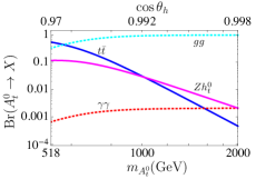
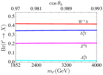
Figure 1: The branching ratios of $A^{0}_{t}$ (left panel) and $t^{\prime}$ (right panel) as functions of $m_{A^{0}_{t}}$ and $m_{t^{\prime}}$, respectively. Values of $\cos\theta_{h}$ are also shown in the upper horizontal axes.

From the plot we see that, in the smaller mass region, the $t\bar{t}$ and $gg$ modes are the dominant decay channels, and therefore the main production process is the gluon-gluon fusion (ggF). The 8 TeV LHC cross sections $pp\to A^{0}_{t}\to gg/tt$ for $m_{A^{0}_{t}}\geq 1\,\text{TeV}$ have not seriously been limited by the currently available data yet. It is therefore to be expected that more data from the upcoming Run-II would probe the $A^{0}_{t}$ through these channels. Another interesting channel would be $A^{0}_{t}\to Zh^{0}_{t}$. However, with the updated branching ratio, this channel seems to be rather challenging even at the $\sqrt{s}=14\,\text{TeV}$ LHC with 3000 ${\rm fb}^{-1}$ data due to the small branching ratio in the smaller mass region.

The $t^{\prime}$ quark arises as a mixture of the gauge-eigenstate top and $\chi$-quarks through the diagonalization of the fermion mass matrix in the effective Lagrangian Eq.(8). The explicit expressions of the $t^{\prime}$ couplings and the partial decay widths relevant to the LHC study are listed in [3]. In the right panel of Fig. 1, we plot the branching ratios of the $t^{\prime}$ quark as a function of $m_{t^{\prime}}$. In the same way as the plot for the branching ratios of $A^{0}_{t}$, the corresponding value of $\cos\theta_{h}$ is also shown in the upper horizontal axis. From the figure we read off $\text{Br}(t^{\prime}\to W^{+}b)\simeq\text{Br}(t^{\prime}\to h^{0}_{t}t)\simeq 0.4$, $\text{Br}(t^{\prime}\to Zt)\simeq 0.21$ and $\text{Br}(t^{\prime}\to A^{0}_{t}t)\simeq 0.02$. It is worth comparing these values with the branching ratios of the “singlet $t^{\prime}$ quark” in a benchmark model of $t^{\prime}$ quark [21], $\text{Br}(t^{\prime}\to W^{+}b)\simeq 0.5,\text{Br}(t^{\prime}\to Zt)\simeq 0.25,\text{Br}(t^{\prime}\to ht)\simeq 0.25$, for $m_{t^{\prime}}\simeq 2\,\text{TeV}$ [22, 23]. It is interesting to note that $\text{Br}(t^{\prime}\to h^{0}_{t}t)$ in the present model is by about $40\,\%$ larger than that in the benchmark model. This is essentially due to the large $ht^{\prime}t$ coupling, which is the very consequence of the top quark condensate scenario.

5 Summary

We presented the Top Mode pseudo Nambu-Goldstone boson Higgs (TMpNGBH) model which has recently been proposed as a variant of the top quark condensate model in light of the 125 GeV Higgs boson discovered at the LHC. We also discussed the vacuum alignment problem of TMpNGBH model based on the one-loop effective Lagrangian for the NGB sector, taking into account all the explicit breaking effects, including electroweak gauge interactions and four fermion interactions responsible for the top-seesaw mechanism. We found that the correct vacuum is determined by the configuration which minimizes the one-loop effective potential. It was found that the true vacuum is parameterized by $\cos\theta_{h}$, and a non-zero value of $\cos\theta_{h}$ realizes the EWSB phase with the appropriate breaking scale. Furthermore, we also discussed the phenomenological implications of the TMpNGBH model on the vacuum aligned at the one-loop level.

References

- [1] H. S. Fukano, M. Kurachi, S. Matsuzaki and K. Yamawaki, Higgs boson as a top-mode pseudo-Nambu-Goldstone boson, Phys.Rev. D90, p. 055009 (2014).
- [2] H. S. Fukano and S. Matsuzaki, Top-mode pseudo-Nambu-Goldstone bosona at the LHC, Phys.Rev. D90, p. 015005 (2014).
- [3] H. S. Fukano, M. Kurachi and S. Matsuzaki, Vacuum Alignment of the Top-Mode Pseudo-Nambu-Goldstone Boson Higgs Model, Phys.Rev. D91, p. 115005 (2015).
- [4] G. Aad et al., Observation of a new particle in the search for the Standard Model Higgs boson with the ATLAS detector at the LHC, Phys.Lett. B716, 1 (2012).
- [5] S. Chatrchyan et al., Observation of a new boson at a mass of 125 GeV with the CMS experiment at the LHC, Phys.Lett. B716, 30 (2012).
- [6] F. Abe et al., Observation of top quark production in collisions, Phys.Rev.Lett. 74, 2626 (1995).
- [7] S. Abachi et al., Observation of the top quark, Phys.Rev.Lett. 74, 2632 (1995).
- [8] K. Olive et al., Review of Particle Physics, Chin.Phys. C38, p. 090001 (2014).
- [9] V. Miransky, M. Tanabashi and K. Yamawaki, Dynamical Electroweak Symmetry Breaking with Large Anomalous Dimension and t Quark Condensate, Phys.Lett. B221, p. 177 (1989).
- [10] V. Miransky, M. Tanabashi and K. Yamawaki, Is the t Quark Responsible for the Mass of W and Z Bosons?, Mod.Phys.Lett. A04, p. 1043 (1989).
- [11] W. A. Bardeen, C. T. Hill and M. Lindner, Minimal Dynamical Symmetry Breaking of the Standard Model, Phys.Rev. D41, p. 1647 (1990).
- [12] H.-C. Cheng, B. A. Dobrescu and J. Gu, Higgs mass from compositeness at a multi-TeV scale, JHEP 1408, p. 095 (2014).
- [13] Y. Nambu and G. Jona-Lasinio, Dynamical Model of Elementary Particles Based on an Analogy with Superconductivity. 1., Phys.Rev. 122, 345 (1961).
- [14] B. A. Dobrescu and C. T. Hill, Electroweak symmetry breaking via top condensation seesaw, Phys.Rev.Lett. 81, 2634 (1998).
- [15] R. S. Chivukula, B. A. Dobrescu, H. Georgi and C. T. Hill, Top quark seesaw theory of electroweak symmetry breaking, Phys.Rev. D59, p. 075003 (1999).
- [16] H.-J. He, C. T. Hill and T. M. Tait, Top quark seesaw, vacuum structure and electroweak precision constraints, Phys.Rev. D65, p. 055006 (2002).
- [17] H. S. Fukano and K. Tuominen, A hybrid 4 generation: Technicolor with top-seesaw, Phys.Rev. D85, p. 095025 (2012).
- [18] H. S. Fukano and K. Tuominen, 126 GeV Higgs boson in the top-seesaw model, JHEP 1309, p. 021 (2013).
- [19] M. E. Peskin and T. Takeuchi, A New constraint on a strongly interacting Higgs sector, Phys.Rev.Lett. 65, 964 (1990).
- [20] M. E. Peskin and T. Takeuchi, Estimation of oblique electroweak corrections, Phys.Rev. D46, 381 (1992).
- [21] F. del Aguila, L. Ametller, G. L. Kane and J. Vidal, Vector Like Fermion and Standard Higgs Production at Hadron Colliders, Nucl.Phys. B334, p. 1 (1990).
- [22] J. Aguilar-Saavedra, Identifying top partners at LHC, JHEP 0911, p. 030 (2009).
- [23] J. Aguilar-Saavedra, R. Benbrik, S. Heinemeyer and M. Pérez-Victoria, Handbook of vectorlike quarks: Mixing and single production, Phys.Rev. D88, p. 094010 (2013).