A modified bootstrap percolation on
a random graph coupled with a lattice

Abstract.

In this paper a random graph model $G_{\mathbb{Z}^{2}_{N},p_{d}}$ is introduced, which is a combination of fixed torus grid edges in $(\mathbb{Z}/N\mathbb{Z})^{2}$ and some additional random ones. The random edges are called long, and the probability of having a long edge between vertices $u,v\in(\mathbb{Z}/N\mathbb{Z})^{2}$ with graph distance $d$ on the torus grid is $p_{d}=c/Nd$, where $c$ is some constant. We show that, whp, the diameter $D(G_{\mathbb{Z}^{2}_{N},p_{d}})=\Theta(\log N)$. Moreover, we consider a modified non-monotonous bootstrap percolation on $G_{\mathbb{Z}^{2}_{N},p_{d}}$. We prove the presence of phase transitions in mean-field approximation and provide fairly sharp bounds on the error of the critical parameters.

1. introduction

Bootstrap percolation is a cellular automaton, which has been introduced by Chalupa, Leath, and Reich [12] as a process on the Bethe lattice where every vertex can be in active or inactive state. Initially, a vertex is active with some probability independently of the state of other vertices. The process is defined so that an active vertex stays active forever, while the state of an inactive vertex at each step is determined following an update rule based on the states of its neighbors. It is said that the process percolates if all the vertices eventually become active.

Bootstrap percolation on lattices has been extensively investigated in the last decades. It has been shown under a broad range of conditions that there is a critical initialization probability such that above this probability there is percolation, while there is no percolation below this critical probability. The corresponding effect is called phase transition, which occurs at the critical probability. The main goal is to derive conditions for the critical probability as the function of the properties of the lattice and the update rule. For bootstrap percolation on the two-dimensional square infinite lattice with 2-neighbor update rule, i.e., a site becomes active if at least 2 of its neighbors are active, the first result is due to van Enter [30] who proved that the critical probability is zero. This result was generalized to all dimensions by Schonmann [27]. It was shown that for the $r$-neighbor rule in $d$ dimensions the critical probability is 0 if $r\leq d$ and 1 otherwise. The finite volume (metastabilty) behaviour was investigated by Aizenman and Lebowitz [2] and the threshold function for the critical probabilty $p_{c}([n]^{d},r)$ for the finite $d$-dimensional lattice with $r$-neighbor rule has been identified up to a constant factor by Cerf and Manzo [11] for all $d\geq r$. For $d=r=2$ the sharp threshold

(1.1) $$p_{c}([n]^{2},2)=\frac{{\pi}^{2}}{18\log n}+o\left(\frac{1}{\log n}\right)$$

has been proved by Holroyd [20]. Surpisingly, this result contradicted to numerical predictions, which were apparently due to slow convergence. Finally, Balogh, Bollobás, Duminil-Copin, and Morris [5] derived sharp threshold for $p_{c}([n]^{d},r)$ for all $d\geq r$.

It is of interest to analyze a modified model by relaxing the original condition requiring that an active vertex stays active forever. This leads to a broader class of modified non-monotonous bootstrap percolation when most of techniques used in (monotonous) bootstrap percolation cannot be applied. There are some results for models with non-monotonous bootstrap percolation. Coker and Gunderson [14] considered bootstrap percolation with a modified $k$-threshold rule. In their case, an inactive vertex becomes active if it has at least $k$ active neighbors, while an active vertex with no active neighbors becomes inactive. The last condition allowed to generalize techniques previously used for bootstrap percolation and find sharp thresholds for the critical probability of initial activations so that all vertices eventually become active.

Recently, bootstrap percolation has been considered on the Erdős-Rényi random graph $G_{n,p}$ in [21], where a theory has been developed regarding the size $a$ of the set of initially active sites. Results include sharp threshold for phase transition for parameters $p$ and $a$, and the time $t$ required to the termination of the bootstrap percolation process. Turova and Vallier [29] considered bootstrap percolation on the combination of the random graph $G_{n,p}$ and the $n$-cycle, where random edges are added between any pair of vertices of the $n$-cycle with probability $p$ independently of each other. Starting with $a$ active vertices, they analyzed when the percolation process terminates. Sharp thresholds for phase transition for parameters $p$ and $a$ were derived. In particular, it was shown that for a range of the parameters, the process percolates on the combined graph but not on the random graph $G_{n,p}$ without local edges. In [16] the authors considered bootstrap percolation process on $G_{n,p}$ with vertices of two different types.

There has been extensive work on studying random graphs of large order, which have relatively small diameter. For example, Bollobás and Chung [9] showed that adding a random matching to the $n$-cycle reduces its $\lfloor n/2\rfloor$ diameter to $(1+o(1))\log_{2}n$. The so called $n$-cycle long-range percolation graph has been considered in [7] where the probabilities of added random edges decay polynomially with the distance between the corresponding pairs of vertices. It was shown that the diameter of this graph is of the order of $\log n$, assuming that the parameters are constrained to a certain parameter region. The combination of a finite $d$-dimensional grid $[n]^{d}$ with random edges (decreasing in distance) added has been considered by Coppersmith, Gamarnik and Sviridenko [15]. They showed that under certain conditions on the dimension and probability $p$, the diameter is either $\Theta(\log n)$ or $n^{\eta}$, where the power coefficient $\eta$ satisfies $0<\eta<1$.

Watts and Strogatz [31] introduced the ”small world” network. The edges of a so-called ring lattice with $k$ edges per vertex are rewired with probability $p$. This construction leads to the drastic reduction of the network diameter, and it allows to ’tune’ the graph between regularity ($p=0$) and disorder ($p=1$). A different version of the ”small world” model has been described by Newman and Watts [26]. Here, an $n$-cycle is considered and the edges of the cycle are fixed. In contrast to the original formulation, however, in [26] random edges are added with some probability instead of rewiring the edges of the cycle, which significantly reduces the graph diameter, too. Since then there has been a high interest in the small world phenomenon in mathematical and other communities [3]. Scaling behavior and phase transitions in inhomogeneous random graphs have been also investigated, see, for example [10].

In this paper we consider a stochastic process of activation propagation over the random graph which combines lattice $\mathbb{Z}^{2}$ with additional random edges that depend on the distance between vertices. A similar graph has been studied, by, e.g., Aizenman, Kesten and Newman [1], the so-called long-range percolation graph. In that model a pair of sites of the $d$-dimensional lattice $\mathbb{Z}^{d}$ is connected (or a bond is occupied) with probability that depends on the graph distance. In the present work, we change the way probabilities are defined over the long-range percolation graph, to get a sparser graph with respect to long edges. We consider a random graph $G$ that is built as follows. We start with the $\mathbb{Z}^{2}$ lattice over a $(N+1)\times(N+1)$ grid, and we assume periodic boundary conditions. Thus, we have a torus $\mathbb{T}^{2}=(\mathbb{Z}/N\mathbb{Z})^{2}$, with the short notation $\mathbb{Z}^{2}_{N}$. The set of vertices of $G$ consists of all vertices of $\mathbb{Z}^{2}_{N}$, in total $N^{2}$ vertices. All the edges from the torus grid $\mathbb{Z}^{2}_{N}$ are included in the graph $G$. In addition, we introduce random edges as follows. For every pair of vertices we assign an edge with probability that depends on the graph distance $d$ between the two vertices, i.e., $d$ is the length of the shortest path between the given pair of vertices in the torus grid. Accordingly, the probability of a long edge is described as follows:

(1.2) $$\mathbb{P}\left((u,v)\in E(G)\right)=p_{d}=\frac{c}{N}\times{d^{-\alpha}}\qquad\text{when}\quad\operatorname{dist}(u,v)=d,$$

where $c$ and $\alpha$ are positive constants, $d>1$ (no multiple edges are allowed between any pair of vertices) and $N$ is large enough so that each $p_{d}<1$. We assume $\alpha=1$ throughout this study. We will denote this model the $G_{\mathbb{Z}^{2}_{N},p_{d}}$ graph. The edges of the torus are called short edges, while the randomly added ones are called long edges.

The present work is organized as follows: first we describe some properties of the introduced random graph $G_{\mathbb{Z}^{2}_{N},p_{d}}$. We derive bounds on the diameter of this graph and describe its degree distribution using Poisson approximation. The second part of this paper is devoted to the study of an activation process using a modified non-monotonous bootstrap percolation model. First, we consider the critical probability of the activation process and state a few conjectures, and then to simplify the mathematical treatment, we analyze the activation as a stochastic process in mean-field approximation [4]. We derive conditions for phase transitions as a function of the model parameters, including the proportion of long edges $\lambda$ and the $k$-neighbor update rule parameter $k$.

We will use the following standard notation; for non-negative sequences $a_{m}$ and $b_{m}$, $a_{m}=O(b_{m})$ if $a_{m}\leq cb_{m}$ holds for some constant $c>0$ and every $m$; $a_{m}=\Theta(b_{m})$ if both $a_{m}=O(b_{m})$ and $b_{m}=O(a_{m})$ hold; $a_{m}\sim b_{m}$ if $\lim_{m\to\infty}{a_{m}}/{b_{m}}=1$; $a_{m}=o(b_{m})$ if $\lim_{m\to\infty}{a_{m}}/{b_{m}}=0$. A sequence of events $A_{n}$ occurs with high probability, whp, if the probability $\mathbb{P}(A_{n})=1-o(1)$.

2. Properties of $G_{\mathbb{Z}^{2}_{N},p_{d}}$

First notice that the expected number of long edges $E_{\ell}\subseteq E(G_{\mathbb{Z}^{2}_{N},p_{d}})$ is proportional to $N^{2}$.

Claim 1.

$\mathbb{E}(|E_{\ell}|)\sim(2c\ln 2)N^{2}$, i.e., $\displaystyle{\lim_{N\to\infty}\frac{\mathbb{E}(|E_{\ell}|)}{2cN^{2}\ln 2}=1}$.

Proof.

Indeed, the number of vertices $|\Lambda_{d}|$ in $\mathbb{Z}^{2}_{N}$ which are exactly at distance $d$ from a fixed vertex is

$$|\Lambda_{d}|=\begin{cases}4d,&\text{$1\leq d\leq\left\lfloor N/2\right\rfloor$}\\ 4(N-d),&\text{$\left\lfloor N/2\right\rfloor<d\leq N$}\end{cases}$$

for $N$ odd, and

$$|\Lambda_{d}|=\begin{cases}4d,&\text{$1\leq d<N/2$}\\ 4d-2,&\text{$d=N/2$}\\ 4(N-d),&\text{$N/2<d<N$}\\ 1,&\text{$d=N$}\end{cases}$$

for $N$ even. The number of pairs of vertices in $\mathbb{Z}^{2}_{N}$ having distance $d$ is $\frac{N^{2}|\Lambda_{d}|}{2}$. Therefore, for $N$ odd

(2.1) $$\mathbb{E}(|E_{\ell}|) = \sum_{d=2}^{N}\frac{N^{2}|\Lambda_{d}|}{2}\frac{c}{Nd}=\sum_{d=2}^{N/2}\frac{4N^{2}d}{2}\frac{c}{Nd}+\sum_{d=N/2+1}^{N}\frac{4N^{2}(N-d)}{2}\frac{c}{Nd}$$

$$= (2c\ln 2)N^{2}+O(N)\sim(2c\ln 2)N^{2}.$$

For $N$ even a similar computation gives the same result. ∎

2.1. Degree distribution

The degree distribution of a vertex $v\in G_{\mathbb{Z}^{2}_{N},p_{d}}$ with respect to long edges can be approximated by Poisson distribution. Let $W$ be the random variable describing the degree of a particular vertex $v$ considering long edges only. Then clearly, the degree of a vertex $v\in G_{\mathbb{Z}^{2}_{N},p_{d}}$ considering the short edges, too, is $W+4$.

Lemma 1.

The probability that a vertex has degree $k$ considering only the long edges is given by

(2.2) $$\mathbb{P}\left(W=k\right)=\sum_{k_{2}+\ldots+k_{N}=k}\;\;{\prod_{i=2}^{N}{\binom{|\Lambda_{i}|}{k_{i}}\left(\frac{c}{Ni}\right)^{k_{i}}\left(1-\frac{c}{Ni}\right)^{|\Lambda_{i}|-k_{i}}}}.$$

The total variation distance

(2.3) $$d_{TV}\left(\mathcal{L}(W),\mathrm{Po}(\lambda)\right)=\frac{1}{2}\sum_{j\geq 0}|\mathbb{P}(W=j)-\mathbb{P}(Y=j)|=O(1/N),$$

where the random variable $Y$ has Poisson distribution $\mathrm{Po}(\lambda)$, with $\lambda=4c\ln 2$.

Proof.

The probability of the event $A_{i}$ that a vertex has $k_{i}$ edges of length $i$ is clearly

(2.4) $$\mathbb{P}\left(A_{i}\right)=\binom{|\Lambda_{i}|}{k_{i}}\left(\frac{c}{Ni}\right)^{k_{i}}\left(1-\frac{c}{Ni}\right)^{|\Lambda_{i}|-k_{i}}$$

Therefore, the probability that a vertex has degree exactly $k$ is

(2.5) $$\mathbb{P}\left(W=k\right)=\mathbb{P}\left(\bigcup_{k_{2}+\ldots+k_{N}=k}\;\;\bigcap_{i=2}^{N}A_{i}\right)=\sum_{k_{2}+\ldots+k_{N}=k}\;\;{\prod_{i=2}^{N}{\mathbb{P}\left(A_{i}\right)}}\\ =\sum_{k_{2}+\ldots+k_{N}=k}\;\;{\prod_{i=2}^{N}{\binom{|\Lambda_{i}|}{k_{i}}\left(\frac{c}{Ni}\right)^{k_{i}}\left(1-\frac{c}{Ni}\right)^{|\Lambda_{i}|-k_{i}}}}.$$

The last expression is not very convenient to use. However, a standard Poisson approximation can be given using Le Cam’s argument [25], see also e.g. [6]. Pick an arbitrary vertex $v$ and let enumerate the other $N^{2}-5$ vertices by $u_{i}$, $i=1,\ldots,N^{2}-5$, excluding the nearest neighbors, i.e., vertices at distance 1. The long edges that connect the vertex $v$ to other vertices of the graph are independent 0–1 random variables with Bernoulli Be$(p_{i})$ distribution. In other words, let $I_{i}=1$ be the event that there is an edge between vertices $v$ and $u_{i}$, so that $\mathbb{P}(I_{i}=1)=p_{i}$ and $\mathbb{P}(I_{i}=0)=1-p_{i}$, where $p_{i}$ may in general vary for different $i$. Consider now the degree $W=\sum_{i=1}^{N^{2}-5}{I_{i}}$ of the vertex $v$. Let

$$\lambda_{1}=\sum_{i=1}^{N^{2}-5}{p_{i}}=4c\ln 2+O(1/N),$$

where the last equality follows from Eq. (2.1). By triangle inequality,

(2.6) $$d_{TV}\left(\mathcal{L}(W),\text{Po}(\lambda)\right)\leq d_{TV}\left(\mathcal{L}(W),\text{Po}(\lambda_{1})\right)+d_{TV}\left(\text{Po}(\lambda_{1}),\text{Po}(\lambda)\right)$$

The first term, by Le Cam [25], see also [6, Theorem 2.M], is at most

(2.7) $$\sum_{i=1}^{N^{2}-5}{p_{i}^{2}} = \sum_{d=2}^{N}{|\Lambda_{d}|p_{d}^{2}}\leq\sum_{d=1}^{N}{|\Lambda_{d}|p_{d}^{2}}=\sum_{d=1}^{N/2}{4d}\left(\frac{c}{Nd}\right)^{2}$$

$$+ \sum_{d=N/2+1}^{N}{4(N-d)}\left(\frac{c}{Nd}\right)^{2}\leq\sum_{d=1}^{N}{4d}\left(\frac{c}{Nd}\right)^{2}=O\left(\frac{\ln N}{N^{2}}\right).$$

and by Theorem 1.C (i) in [6]

(2.8) $$d_{TV}\left(\text{Po}(\lambda_{1}),\text{Po}(\lambda)\right)=O\left(|\lambda_{1}-\lambda|\right)=O\left(\frac{1}{N}\right).$$

∎

Clearly, Lemma 1 also implies that in Eq. (2.3) each term satisfies $|\mathbb{P}(W=j)-\mathbb{P}(Y=j)|=O(1/N)$.

2.2. The diameter of $G_{\mathbb{Z}^{2}_{N},p_{d}}$

Next we show that the addition of long edges to the torus grid reduces significantly (from linear to logarithmic in the number of vertices) its diameter.

Theorem 1.

There exist constants $C_{1},C_{2}$, which depend on $c$ only, such that for the diameter $D(G_{\mathbb{Z}^{2}_{N},p_{d}})$ the following hold.

$$\lim_{N\rightarrow\infty}\mathbb{P}\left(C_{1}\log{N}\leq D(G_{\mathbb{Z}^{2}_{N},p_{d}})\leq C_{2}\log{N})\right)=1,~{}{\mbox{i}.e.,}~{}D(G_{\mathbb{Z}^{2}_{N},p_{d}})=\Theta(\log N),~{}whp.$$

Proof.

The lower bound is trivial. The expected degree $\mathbb{E}(d(v))$ of a vertex $v$ by Claim 1 is a constant $k=k(c)$. Thus, the expected number of vertices $A_{m}$ we can reach in at most $m\geq 0$ steps from a given vertex $v$ is less than or equal to $1+\sum_{i=1}^{m}k(k-1)^{i-1}$. For $m\geq 3$, this is less than $k^{m}$, and thus, by Markov’s inequality,

(2.9) $$\mathbb{P}(A_{m}\geq N^{2})\leq\frac{\mathbb{E}(A_{m})}{N^{2}}\leq\frac{k^{m}}{N^{2}}.$$

If we choose $m\leq C_{1}\log N$ with $C_{1}$ sufficiently small, the probability in Eq. (2.9) tends to zero, i.e., we cannot reach all vertices of the graph from a given vertex $v$ by a path with at most $C_{1}\log N$ edges. Hence, $C_{1}\log N$ bounds the diameter from below.

To prove the upper bound, partition the vertices of $G_{\mathbb{Z}^{2}_{N},p_{d}}$ into consecutive $k\times k$ blocks $B_{ij},i,j=1,\ldots,\frac{N}{k}$, where $k$ is a constant $k(c)$ to be chosen later. (For simplicity, we will assume that everywhere divisibility holds during the proof; otherwise we let some blocks be $(k+1)\times(k+1)$.) Define the graph $G^{\prime}$ as follows. The vertices are the blocks, and two blocks $B_{i,j}$ and $B_{k,\ell}$, $(1,\leq i,j,k,\ell\leq N/k)$ are connected iff there is a long edge from a vertex of $B_{i,j}$ to a vertex of $B_{k,\ell}$ in $G_{\mathbb{Z}^{2}_{N},p_{d}}$. We obtain a random graph on $N^{2}/k^{2}$ vertices where the edge probabilities can be obtained from the ones of $G_{\mathbb{Z}^{2}_{N},p_{d}}$. For an arbitrary pair of vertices $B_{i,j}$ and $B_{k,\ell}$, the probability of the event $A_{i,j;k,l}$ that they are connected is bounded from below by the probability, that two blocks which are most distant from each other in $\mathbb{Z}^{2}_{N}$ are connected. Therefore, for large $N$,

$$\mathbb{P}(A_{i,j;k,l}) \geq \mathbb{P}(A_{1,1;N/(2k),N/(2k)})=1-\mathbb{P}(\overline{A_{1,1,\frac{N}{2k},\frac{N}{2k}}})\geq 1-(1-p_{N})^{k^{4}}$$

$$= 1-\left(1-\frac{c}{N^{2}}\right)^{k^{4}}\geq 1-e^{-ck^{4}/N^{2}}\geq ck^{4}/2N^{2}.$$

For the second inequality we picked the two most distant vertices from each block, and the last one follows from $e^{x}\leq 1+x/2$ for $x<0$ sufficiently close to $0$. Consequently, we can couple the random graph $G^{\prime}$ with a random graph $G^{\prime\prime}\subseteq G^{\prime}$ where edges appear independently with probability $ck^{4}/2N^{2}$, i.e., $G^{\prime\prime}$ is an Erdős-Rényi random graph $G_{n,p}$ with $n=N^{2}/k^{2}$ and $p=ck^{4}/2N^{2}$.

By, e.g., Theorem 9.b in the seminal paper of Erdős and Rényi [17] there is a constant $c_{1}$ such that in the Erdős-Rényi random graph $G_{n,p}$ with $p=c_{1}/n$ there is a giant component on at least, say, $n/2$ vertices, whp. Choosing

$$k\geq(2c_{1}/c)^{1/2}$$

we get that the edge probability in $G^{\prime\prime}$ is

$$ck^{4}/2N^{2}\geq c_{1}k^{2}/N^{2},$$

and thus $G^{\prime\prime}$ will contain a giant component on at least $N^{2}/2k^{2}$ vertices, whp. The diameter of the giant component of $G_{n,p}$ with $p=c_{1}/n$ is known to be of order $O(\log n)$, whp. (See, e.g. Table 1 in [13].)

First, assume that vertices $u,v\in G_{\mathbb{Z}^{2}_{N},p_{d}}$ are contained in blocks $B(u)$ and $B(v)$ which are vertices of the giant component in $G^{\prime\prime}$. Find the shortest path, say, $B(u)=B(x_{0}),B(x_{1}),B(x_{2}),\ldots,B(x_{m})=B(v)$, between $B(u)$ and $B(v)$ in $G^{\prime\prime}\subseteq G^{\prime}$. Let $(x_{0},x_{1})$, $(x_{1}^{\prime},x_{2})$, $(x_{2}^{\prime},x_{3})$, …, $(x_{m-1}^{\prime},x_{m})$, $x_{i},x_{i}^{\prime}\in B(x_{i})$ be the edges in $G_{\mathbb{Z}^{2}_{N},p_{d}}$ inducing this path in $G^{\prime}$.

Now go from $u$ to $x_{0}$ in $B(u)$ along short ($\mathbb{Z}^{2}$) edges. Jump from $x_{0}$ to $x_{1}$. Then go from $x_{1}$ to $x_{1}^{\prime}$ in $B(x_{1})$ along short edges. Jump from $x_{1}$ to $x_{2}^{\prime}$, and so on. The total length of the path from $u$ to $v$, will be at most

$$m+2k(m+1)\leq(2k+1)(m+1).$$

Indeed, we make $m$ jumps, and within each block we make at most $2k$ steps along short edges. Since $m=O(\log N)$, whp, the case when $u$ and $v$ are inside blocks that belong to the giant component in $G^{\prime\prime}$ is finished.

Next we show that, whp, every vertex $v\in G_{\mathbb{Z}^{2}_{N},p_{d}}$ is close to some block $B$ of the giant component in $G^{\prime\prime}$. Indeed, by symmetry, the set $A$ of vertices in the giant component of $G^{\prime\prime}$ can be any set of vertices of the same size, with the same probability. Therefore, one can regard $A$ as a uniformly random subset on at least half of the vertices in $G^{\prime\prime}$.

For some large constant $D$, the number of vertices with distance at most $D\sqrt{\log_{2}N}$ from a fixed vertex $v$ in $\mathbb{Z}^{2}$ is

$$\sum_{d=1}^{D\sqrt{\log_{2}N}}4d\geq 4D^{2}\log_{2}N,$$

i.e., this neighborhood contains a vertex from at least

$$\frac{4D^{2}\log_{2}N}{k^{2}}$$

blocks. Since $A$ contains at least half of the vertices in $G^{\prime\prime}$, the probability that none of those blocks is in $A$ is

$$\leq 2^{-\frac{4D^{2}\log_{2}N}{k^{2}}}=N^{-4D^{2}/k^{2}}.$$

Therefore, the probability that there is a vertex $v\in G_{\mathbb{Z}^{2}_{N},p_{d}}$ for which there is no vertex $u$ within distance $D\sqrt{\log_{2}N}$ such that $B(u)\in A$ is

$$\leq N^{2}\cdot N^{-4D^{2}/k^{2}}<N^{-2},$$

assuming that $D$ is large enough.

Now, consider two arbitrary vertices $u,v\in G_{\mathbb{Z}^{2}_{N},p_{d}}$. If one or neither of them is in a block from $A$, then, whp, each of them can reach a block from $A$ within $D\sqrt{\log_{2}N}$ steps in $\mathbb{Z}^{2}$, and then proceed as in case $B(u),B(v)\in A$. Since the number of additional steps whp is $O(\sqrt{\log N})$, the proof is finished. ∎

3. Activation process on the random graph $G_{\mathbb{Z}^{2}_{N},p_{d}}$

Now we introduce a stochastic process on the graph we have just built. Each vertex is described by its state, which can be either active or inactive. The state of the vertex changes during the process according to a rule specified next. We define a potential function $\chi_{v}(t)$ for each vertex $v$ such that $\chi_{v}(t)=1$ if vertex $v$ is active at time $t$, and $\chi_{v}(t)=0$ if $v$ is inactive. Let $A(t)$ denote the set of all active vertices at time $t$, thus $A(t)=\{v\in V(G_{\mathbb{Z}^{2}_{N},p_{d}})\bigm{|}\chi_{v}(t)=1\}$.

At the beginning, let $A(0)$ be a random subset of vertices with each vertex active with probability $p$, independently of all other vertices, and the corresponding distribution we denote by $\mathbb{P}_{p}$. Each vertex may change its activity based on the states of its neighbors, according to the rule ${\mathcal{R}_{k}}$

(3.1) $$\chi_{v}(t+1)=\mathbbm{1}\left(\sum_{u\in N(v)}{\chi_{u}(t)}\geq k\right),$$

where $\mathbbm{1}$ is the indicator function and $N(v)$ denotes the subsets of vertices in the closed neighborhood of the vertex $v$, i.e., the vertex $v$ and its neighbors. Here $k$ is a nonnegative integer that specifies the threshold required for the vertex to be in the active state at the next step.

According to Eq. (3.1) we have a $k$-neighbor update rule, i.e., a vertex will be active at the next time step if it has at least $k$ active neighbors including itself. Observe, that the set of active vertices does not necessarily grow monotonically during the activation process in the present modified bootstrap percolation model, in contrast to usual bootstrap percolation.

The set $A$ is said to percolate with respect to rule ${\mathcal{R}_{k}}$, if eventually all vertices in $G_{\mathbb{Z}^{2}_{N},p_{d}}$ get activated and stay so. The critical probability $p_{c}$ for $k\leq 5$ is defined as

(3.2) $$p_{c}\left(G_{\mathbb{Z}^{2}_{N},p_{d}},{\mathcal{R}_{k}}\right)=\inf\{p:~{}\mathbb{P}_{p}~{}(A(0)~{}percolates)\geq 1/2\}.$$

Notice, that for $k\geq 6$, whp, even $A(0)=V(G_{\mathbb{Z}^{2}_{N},p_{d}})$ does not percolate. Indeed, whp, the number of vertices with degree determined by long edges equals to zero is $>e^{-\lambda}N^{2}/2$. That is, even if we initially activate all of the vertices, those with degrees determined by long edges equal to zero will deactivate in the first step and stay so forever.

4. Percolation and density

The pretty straightforward analysis of the activation process in terms of percolation is given as follows.

Proposition 1.

For $0\leq k\leq 2$ and $\lambda\geq 0$, whp, $p_{c}=o(1)$; for $3\leq k\leq 5$ and $\lambda\geq 0$, whp, $p_{c}=1-o(1)$.

Proof.

Cases $k=0$ and $k=1$ are trivial. Even if we start the activation with a single vertex, it will fully percolate.

In the case $k=2$, it is enough to show that the statement holds with $\lambda=0$, since the vertices will get activated even easier after adding long edges.

First notice, that in this case only isolated active vertices can get inactive. Indeed, if an active vertex $v$ is connected to some other active one, by the activation rule it will stay so forever.

Now, let $A^{\prime}(0)\subset A(0)$ be the subset of initially activated, non isolated vertices. If we start the process with $A^{\prime}(0)$, once a vertex get activated, it will stay so forever. Indeed, if a vertex is activated, it is added to an active component, and therefore, will not be isolated. Therefore, starting the process with $A^{\prime}(0)$ it will be monotone.

It is left to show, that there is a ‘sufficiently large’ random subset $A^{\prime}(0)$. One can easily show this concentrating on matchings in the grid. Indeed, activate the vertices in two rounds, each time with probability $p/2$. Thus each vertex gets active with probability at most $p$. Call vertex strongly active, if it was activated in the first round, and its left neighbour in the second round. Clearly, each vertex is strongly active independently with probability $p^{2}/4$. Using, e.g., theorem of Holroyd (1.1, [20]) cited in the introduction concludes the proof.

To prove the case $k=3$, first partition $V(G_{\mathbb{Z}^{2}_{N},p_{d}})$ into squares ($C_{4}$-s) with respect to grid edges (ignoring leftovers if $N$ is odd). Notice, that if no vertex of a $C_{4}$ is initially activated and neither of them has long edges, then the vertices of the $C_{4}$ will never get activated. The probability of this event for a given $C_{4}$ is $\sim e^{-4\lambda}(1-p)^{4}$, assuming an initial activation probability $p$. If follows, e.g. using Chebyshev’s inequality, that whp, at least $e^{-4\lambda}(1-p)^{4}N^{2}/5$ of the vertices will never be active, i.e., a positive fraction. The cases $k=4$, $5$ clearly follow from the case $k=3$. ∎

4.1. The case $k=3$

The evolution of the density, i.e., the behaviour of the random variable $\hat{\rho}_{t}=\hat{\rho}_{t}(N,\lambda,p)=|A(t)|/N^{2}$ as a function of $t$, is particularly interesting in the case $k=3$; in this subsection we consider only this case. In usual bootstrap percolation, where the process is monotone, for an arbitrary initial configuration $A(0)$ of active vertices a final configuration $FC(A(0))$ is always reached. This is not necessarily true in our case, where oscillations may occur for ever, as shown by the following example.

Example 1.

Let $N$ be divisible by 4. Suppose first that there are no long edges, so the graph is $\mathbb{Z}^{2}_{N}$, and suppose that the initial configuration $A(0)$ is a checkerboard pattern where a vertex $(i,j)$ is active if and only if $i+j$ is even. Then the set of active vertices will oscillate, with $A(2n)=A(0)$ and $A(2n+1)=\mathbb{Z}^{2}_{N}\setminus A(0)$ for all $n$. In this example, $|A(t)|$ is constant, but we can modify it by adding some long edges as follows:

Assume that there is a long edge between $(4i,4j)$ and $(4(i+1),4j)$ for all $i,j\in\mathbb{Z}$, but no others. (All coordinates are mod $N$; recall that $N$ is divisible by $4$.) Then, with the same checkerboard initial configuration, the vertices $(4i,4j)$ stay active forever, while the others oscillate as before. Hence, $\hat{\rho}_{t}$ oscillates with $\hat{\rho}_{2n}=1/2$ and $\hat{\rho}_{2n+1}=9/16$.

We believe that global oscillations as exemplified in Example 1 occur with very small probability when $N$ is large. However, there will whp be local oscillations, as shown by the following example.

Example 2.

Consider the box $Q=[-2,6]\times[-2,6]$; we partition $Q=Q_{\mathsf{c}}\cup Q_{\mathsf{i}}\cup Q_{\mathsf{o}}$ where $Q_{\mathsf{c}}=[0,4]\times[0,4]$ (the core), $Q_{\mathsf{i}}=([-1,5]\times[-1,5])\setminus Q_{\mathsf{c}}$ (the inner rim) and $Q_{\mathsf{o}}=Q\setminus Q_{\mathsf{i}}$ (the outer rim). We say that $Q$ is special if there are long edges joining each of the four corners of the core, i.e., $(0,0)$, $(0,4)$, $(4,0)$, $(4,4)$, to two vertices in the outer rim, but no other long edges with an endpoint in $Q$.

Suppose that $Q$ is special, and that in the initial configuration $A(0)$, every vertex in the outer rim is active, but no vertex in the inner rim, while a vertex $(i,j)$ in the core is active if and only if $i+j$ is even. (Cf. Example 1.) Then, the vertices in the outer and inner rims of $Q$ will stay frozen as they are for ever, and so will the four corners of the core, while the other vertices in the core will oscillate as in Example 1. Hence the total number of active vertices in $Q$ will oscillate between 45 and 48 (note that $|Q_{\mathsf{c}}|=25$ and $|Q_{\mathsf{o}}|=32$).

Partition $V(G_{\mathbb{Z}^{2}_{N},p_{d}})$ into $9\times 9$ boxes $Q_{k}$ (ignoring possible leftovers). Each $Q_{k}$ is a translate of $Q$, and we say that $Q_{k}$ is special if the long edges with an endpoint in $Q_{k}$ are such that $Q_{k}$ is a translate of a special $Q$. For a given $\lambda>0$, each box $Q_{k}$ is special with some probability $p_{s,N}$ converging to some $p_{s}>0$ as $N\to\infty$. Hence the expected number of special boxes is $\sim p_{s}N^{2}/81$, and it follows easily using Chebyshev’s inequality that whp the number of special boxes is at least $(p_{s}/100)N^{2}$.

If $Q_{k}$ is a special box, then the initial configuration for $Q$ discussed above translates to an initial configuration of $Q_{k}$ such that the number of active vertices in $Q$ oscillates. For any fixed initial activation probability $p$, this initial configuration of $Q_{k}$ has a certain positive probability, and by independence and the law of large numbers, whp a positive fraction of all special boxes will have this initial configuration, and will thus oscillate.

Consequently, whp at least a fixed positive fraction of all vertices participate for ever in local oscillations.

However, while local oscillations as in Example 2 involve many vertices, we believe that typically, there is no global syncronization and that therefore the many local oscillations to a large extent cancel each other, so that the oscillations in $\hat{\rho}_{t}$ typically are small. To make this precise, define the random variables $\overline{\rho}(N,\lambda,p)=\limsup_{t\to\infty}\hat{\rho}_{t}$ and $\underline{\rho}(N,\lambda,p)=\liminf_{t\to\infty}\hat{\rho}_{t}$ (depending on the graph $G_{\mathbb{Z}^{2}_{N},p_{d}}$ and $A(0)$).

Conjecture 1.

For every fixed $\lambda\geq 0$ and initial probability $0<p<1$, there is a non-random limiting density $\hat{\rho}_{\lim}(\lambda,p)$ such that both $\overline{\rho}(N,\lambda,p)$ and $\underline{\rho}(N,\lambda,p)$ converge in probability to $\hat{\rho}_{\lim}(\lambda,p)$ as $N\to\infty$, i.e., for every $\varepsilon>0$,

$$\mathbb{P}(|\overline{\rho}(N,\lambda,p)-\hat{\rho}_{\lim}(\lambda,p)|>\varepsilon)\to 0,\qquad\mathbb{P}(|\underline{\rho}(N,\lambda,p)-\hat{\rho}_{\lim}(\lambda,p)|>\varepsilon)\to 0.$$

The argument in the proof of Proposition 1 shows that if $\delta=e^{-4\lambda}(1-p)^{4}/5$, then whp $\hat{\rho}_{t}<1-\delta$ for all $t$, and the same argument shows that whp $\hat{\rho}_{t}>\delta$ for all $t$. Hence, whp $\delta\leq\overline{\rho}(N,\lambda,p)\leq 1-\delta$ and $\delta\leq\underline{\rho}(N,\lambda,p)\leq 1-\delta$, and if Conjecture 1 is true, then $0<\hat{\rho}_{\lim}(\lambda,p)<1$, for every $\lambda\geq 0$ and $0<p<1$.

If we consider expectations instead of random variables, note first that Fatou’s lemma implies $\liminf_{t\to\infty}\mathbb{E}\hat{\rho}_{t}\geq\mathbb{E}\underline{\rho}(N,\lambda,p)$ and $\limsup_{t\to\infty}\mathbb{E}\hat{\rho}_{t}\leq\mathbb{E}\overline{\rho}(N,\lambda,p)$. Moreover, if Conjecture 1 holds, then dominated convergence implies $\mathbb{E}\overline{\rho}(N,\lambda,p)\to\hat{\rho}_{\lim}(\lambda,p)$ and $\mathbb{E}\underline{\rho}(N,\lambda,p)\to\hat{\rho}_{\lim}(\lambda,p)$ as $N\to\infty$, and thus

$$\lim_{N\to\infty}\limsup_{t\to\infty}\mathbb{E}\hat{\rho}_{t}=\hat{\rho}_{\lim}(\lambda,p)$$

and similarly for $\liminf$.

In the special case $\lambda=0$, the graph $G_{\mathbb{Z}^{2}_{N},p_{d}}=\mathbb{Z}^{2}_{N}$ is regular and each closed neighborhood has 5 elements. It follows that for $k=3$, there is a symmetry between active and inactive vertices in the update rule, and consequently, if we replace any initial set $A(0)$ by its complement, each $A(t)$ is replaced by its complement $\mathbb{Z}_{N}^{2}\setminus A(t)$. It follows that

$$\rho_{t}(N,0,1-p)\overset{\mathrm{d}}{=}1-\rho_{t}(N,0,p)$$

(where $\overset{\mathrm{d}}{=}$ means equality in distribution), and thus $\overline{\rho}(N,0,1-p)\overset{\mathrm{d}}{=}1-\underline{\rho}(N,0,p)$. Consequently, if Conjecture 1 holds, then

$$\hat{\rho}_{\lim}(0,1-p)=1-\hat{\rho}_{\lim}(0,p),$$

and in particular,

$$\hat{\rho}_{\lim}(0,0.5)=0.5.$$

We believe that the limiting density is less than the initial probability if $p<0.5$ and greater than the initial probability if $p>0.5$:

Conjecture 2.

For $0<p<0.5$,  $\hat{\rho}_{\lim}(0,p)<p$, and for $0.5<p<1$,   $\hat{\rho}_{\lim}(0,p)>p$.

We believe that, furthermore, similar ‘critical’ initial probabilities, i.e., where the evolution of the density changes from decreasing to increasing, do exist for all $\lambda$.

Conjecture 3.

For arbitrary $\lambda\geq 0$ there is a $0<p^{(crit)}_{in}(\lambda)<1$, such that $\displaystyle{\hat{\rho}_{\lim}(\lambda,p^{(crit)}_{in}(\lambda))=p^{(crit)}_{in}(\lambda)}$. Moreover, if $0<p<p^{(crit)}_{in}(\lambda)$, then $\hat{\rho}_{\lim}(\lambda,p)<p$, and if $p^{(crit)}_{in}(\lambda)<p<1$, then $\hat{\rho}_{\lim}(\lambda,p)>p$.

Numerical results shown in Figure 1 support our conjectures.

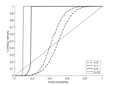
Figure 1. Numerical experiments for the (conjectured) limiting density as function of initial probability with $N=100,$ $k=3$, and $\lambda=10,~{}5,~{}1,~{}0$. The graphs of the functions clearly show, that for $\lambda_{1}>\lambda_{2}$,   the numerical values $\hat{\rho}^{num}_{\lim}(\lambda_{1},x)<\hat{\rho}^{num}_{\lim}(\lambda_{2},x)$, for every $x\in[0,1]$, i.e., as $\lambda$ grows the graphs are more and more squeezed to the $y$ axis. For more details about simulations see Appendix.

5. Mean-field approximation

In order to get some more information on the evolution of the density, we consider the mean-field (MF) approximation of the activation process on $G_{\mathbb{Z}^{2}_{N},p_{d}}$. In the mean field approximation, instead of taking specific fixed neighbors of a given node, we sample a new set of neighbors at each step [4]. This implies that the MF approximation does not depend on the topology of the torus, rather it is completely described by the degree distribution, and the transition probabilities from one state to another depend only on the number of active nodes. The MF approximation means that the results derived here are obtained in the case when the activations and degrees of the various nodes are well-mixed; hence we ignore any dependencies between activation and vertex degrees, as well as any dependencies between the state of a vertex and the state of its neighbors. MF approximations are widely used in various physical models [8, 28], including systems with long-range interactions and spin glasses near critical state. In our model, we also assume that the vertices are activated independently of each other, ignoring the small dependencies between degrees and activities for different vertices.

5.1. Basic concepts

The mean-field density $\rho_{t}$ is defined as follows. Start with $\rho_{0}=\hat{\rho}_{0}\approx p_{in}$. Recall that $\deg(v)$ denotes the degree with respect to the long edges only, so the total degree of a vertex $v$ is $\deg(v)+4$. $\rho_{t}$ is given by the following stochastic recursion

(5.1) $$N^{2}\rho_{t+1}=\operatorname{Bin}(N^{2}\rho_{t},f^{+}(\rho_{t}))+\operatorname{Bin}(N^{2}(1-\rho_{t}),f^{-}(\rho_{t})),$$

where

(5.2) $$f^{+}(x) =\sum_{n=4}^{N^{2}-1}\mathbb{P}\left(\deg(v)=n-4\right)\sum_{i=k}^{n+1}\binom{n}{i-1}x^{i-1}(1-x)^{n-i+1},$$

(5.3) $$f^{-}(x) =\sum_{n=4}^{N^{2}-1}\mathbb{P}\left(\deg(v)=n-4\right)\sum_{i=k}^{n}\binom{n}{i}x^{i}(1-x)^{n-i}.$$

Lemma 2.

Under the mean-field assumptions for the defined process on $G_{\mathbb{Z}^{2}_{N},p_{d}}$, $\rho_{t}$ is a Markov process describing the probability that a given vertex $v$ is active at $t$, i.e., $\rho_{t}$ approximates the density $\hat{\rho}_{t}$. Moreover, given $\rho_{t}$, $\rho_{t+1}$ has mean $f(\rho_{t})$ and variance $g(\rho_{t})/N^{2}$ where

(5.4) $$f(x) =xf^{+}(x)+(1-x)f^{-}(x),$$

(5.5) $$g(x) =xf^{+}(x)(1-f^{+}(x))+(1-x)f^{-}(x)(1-f^{-}(x)).$$

Proof.

At the beginning, for a given initialization probability $p_{in}$, $\rho_{0}=\hat{\rho}_{0}\approx p_{in}$ since vertices are initialized independently at random. Under MF assumptions the state of each vertex at time $t$ is a Bernoulli random variable with parameter $\rho_{t}$; furthermore, different vertices are regarded as independent. The rest of the lemma follow immediately from (5.1)–(5.3). ∎

Remark 1.

In our model, the activation of a vertex is deterministic given the number of active vertices in the closed neighborhood. More generally, one can consider a model where an active (inactive) vertex with $i$ active neighbors is activated with some probability $p_{i}^{+}$ ($p_{i}^{-}$), where $p_{i}^{\pm}$ are some given probabilities. In this more general case, (5.2)–(5.3) become

(5.6) $$f^{+}(x) =\sum_{n=4}^{N^{2}-1}\mathbb{P}\left(\deg(v)=n-4\right)\sum_{i=1}^{n+1}p_{i}^{+}\binom{n}{i-1}x^{i-1}(1-x)^{n-i+1},$$

(5.7) $$f^{-}(x) =\sum_{n=4}^{N^{2}-1}\mathbb{P}\left(\deg(v)=n-4\right)\sum_{i=0}^{n}p_{i}^{-}\binom{n}{i}x^{i}(1-x)^{n-i}.$$

Lemma 2 shows that the conditional variance of $\rho_{t+1}$ is $g(\rho_{t})/N^{2}=O(N^{-2})$, since $g\in[0,1]$ for any $\rho_{t}\in[0,1]$; thus $\rho_{t+1}$ is well concentrated for large $N$, and we can approximate $\rho_{t+1}$ by the mean $f(\rho_{t})$.

The function $f(\cdot)$ given by (5.4) can be simplified to

(5.8) $$\begin{split}f(x)&=xf^{+}(x)+(1-x)f^{-}(x)\\ &=\sum_{n=4}^{N^{2}-1}\mathbb{P}\left(\deg(v)=n-4\right)\sum_{i=k}^{n+1}\binom{n}{i-1}x^{i}(1-x)^{n-i+1}\\ &\qquad+\sum_{n=4}^{N^{2}-1}\mathbb{P}\left(\deg(v)=n-4\right)\sum_{i=k}^{n}\binom{n}{i}x^{i}(1-x)^{n-i+1}\\ &=\sum_{n=4}^{N^{2}-1}\mathbb{P}\left(\deg(v)=n-4\right)\left(\sum_{i=k}^{n+1}\binom{n+1}{i}x^{i}(1-x)^{n-i+1}\right).\end{split}$$

This can also be seen directly. Namely, if $v$ has $n-4$ long edges, the closed neighborhood of $v$ contains $n+1$ vertices, of which $k$ have to be active for activation of $v$, and in the MF approximation, these $n+1$ vertices are active independently of each other.

In Section 2.1 we showed that the degree distribution can be approximated by Poisson distribution $\mathrm{Po}(\lambda)$. We use this fact to approximate $f(x)$. Consider the function

(5.9) $$\bar{f}(x)=\bar{f}_{k}(x)=\sum_{n=4}^{\infty}\frac{e^{-\lambda}\lambda^{n-4}}{(n-4)!}\sum_{i=k}^{n+1}\binom{n+1}{i}x^{i}(1-x)^{n-i+1}.$$

The difference between $f(x)$ and $\bar{f}(x)$ can be bounded by

(5.10) $$|f(x)-\bar{f}(x)|\leq\sum_{n=4}^{\infty}\left|\mathbb{P}\left(\deg(v)=n-4\right)-\frac{e^{-\lambda}\lambda^{n-4}}{(n-4)!}\right|\sum_{i=k}^{n+1}\binom{n+1}{i}x^{i}(1-x)^{n-i+1}\\ \leq\sum_{n=4}^{\infty}\left|\mathbb{P}\left(\deg(v)=n-4\right)-\frac{e^{-\lambda}\lambda^{n-4}}{(n-4)!}\right|=O\left(\frac{1}{N}\right)$$

where the last equality follows from Lemma$~{}1$.

5.2. Derivation of criticality for various $k$ values

We assume for simplicity that $k$ is at most $5$ in the present study.

We rewrite $\bar{f}=\bar{f}_{k}$ defined in (5.9) as

(5.11) $$\bar{f}_{k}(x)=\sum_{n=0}^{\infty}\frac{e^{-\lambda}\lambda^{n}}{n!}\left(\sum_{i=k}^{n+5}\binom{n+5}{i}x^{i}(1-x)^{n+5-i}\right)=\mathbb{P}[\operatorname{Bin}(\deg(v)+5,x)\geq k],$$

where random variable $\deg(v)\sim\mathrm{Po}(\lambda)$.

The critical probabilities in the mean-field approximation are given by the solutions to the fixed point equation $x=f(x)$, where the solutions of this equation are called fixed points. This approach is based on the observation that the critical behavior of the original system often occurs near the unstable fixed points of mean-field approximation [8, 28]. For a discrete time dynamical system, a fixed point is called stable if it attracts all the trajectories that start from some neighborhood of the fixed point. Otherwise, a fixed point is unstable. If $f(x)$ is continuously differentiable in an open neighborhood of a fixed point $x_{0}$, a sufficient condition for $x_{0}$ to be stable or unstable is $|f^{\prime}(x_{0})|<1$ or $|f^{\prime}(x_{0})|>1$, respectively; see, e.g., [19].

Proposition 2.

Let $\bar{f}_{k}(x):[0,1]\rightarrow[0,1]$ be the family of maps for $k=0,\ldots,5$ defined by (5.11). These maps have the following fixed points for any $\lambda>0$:

• for $k=0$ the only fixed point is $1$ and it is stable.

• for $k=1$ there are two fixed points: $1$ is stable and $0$ is unstable.

• for $k=2,3,4$ there are three fixed points: $0$ and $1$ are stable
  and $x_{k}(\lambda)\in(0,1)$ is unstable;

• a. for $k=5$ there are three fixed points for $\lambda>\ln(5)$: $0$ and $1$ are stable and $x_{5}(\lambda)\in(0,1)$ is unstable;
  b. and there are two fixed points for $\lambda\leq\ln(5)$: $0$ is stable and $1$ is unstable.

Proof.

For $k=0$, the equation $\bar{f}_{0}(x)=x$ reduces to just

(5.12) $$x=1.$$

In this case the fixed point $x=1$ is stable since $\bar{f}^{\prime}_{0}(x)=0$.

For $k=1$, $\bar{f}_{1}(x)=x$ can be written

(5.13) $$(1-x)e^{\lambda x}=(1-x)^{5}.$$

This equation has only two solutions $0$ and $1$ in $[0,1]$, where $0$ is an unstable fixed point since $\bar{f}^{\prime}_{1}(0)=5+\lambda>1$, while $1$ is a stable fixed point because $\bar{f}^{\prime}_{1}(1)=0$.

Now we consider cases (iii) and (iv)-$a$ together. It is easy to see that in these cases $\bar{f}_{k}(0)=0$ and $\bar{f}_{k}(1)=1$. Also easy calculations show that $\bar{f}^{\prime}_{k}(x)$ is given on $(0,1]$ by

(5.14) $$\hskip 36.135pt\bar{f}^{\prime}_{k}(x)=\frac{k}{x}\mathbb{P}[\operatorname{Bin}(\deg(v)+5,x)=k]=\frac{k}{x}\mathbb{P}[\mathrm{Po}(\lambda x)+\operatorname{Bin}(5,x)=k].$$

This function can be rewritten (for any $k\geq 2$) as

(5.15) $$\hskip 36.135pt\bar{f}^{\prime}_{k}(x)=ke^{-\lambda x}x^{k-1}\sum_{i=0}^{\min\{k,5\}}\binom{5}{i}\frac{\lambda^{k-i}(1-x)^{5-i}}{(k-i)!}.$$

In order to see that there exists a solution of $\bar{f}_{k}(x)=x$ on $(0,1)$, note that in case (iii) $\bar{f}^{\prime}_{k}(0)=0$ and $\bar{f}^{\prime}_{k}(1)=0$. In case $k=5$, $\bar{f}^{\prime}_{5}(1)=5e^{-\lambda}$, which is less than 1 if $\lambda>\ln(5)$, while $\bar{f}^{\prime}_{5}(0)=0$ for any $\lambda$. Since function $\bar{f}_{k}(x)$ is continuous there will be at least one solution to $\bar{f}_{k}(x)=x$ on $(0,1)$.

This solution is unique. Assume for the contrary that there exist at least two solutions on $(0,1)$. Since $0$ and $1$ are solutions, Rolle’s theorem implies that the derivative $\bar{f}^{\prime}_{k}(x)-1$ of $\bar{f}_{k}(x)-x$ would have at least three zeros on $(0,1)$. We are going to show that the function $\bar{f}^{\prime}_{k}(x)$ is unimodal on $[0,1]$, and not constant on any interval, which would yield a contradiction. To establish the required property of $\bar{f}^{\prime}_{k}(x)$, we denote the quintic polynomial in (5.15) by $P_{k}(x)$. Clearly, $e^{-\lambda x}$, $x^{k-1}$ are log-concave on $(0,1)$, and $P_{k}(x)$ is strictly log-concave on $(0,1)$, see Appendix. Hence $\bar{f}^{\prime}_{k}(x)$ is strictly log-concave, and therefore it is unimodal, and not constant in any interval.

In the existence argument above we showed that $\bar{f}^{\prime}_{k}(0)=0$ and $\bar{f}^{\prime}_{k}(1)<1$. Therefore, the fixed points $x=0$ and $x=1$ are stable in cases (iii) and (iv)-$a$. This also implies that the unique solution on $(0,1)$ is unstable.

Finally, in case (iv)-$b$, $\bar{f}_{5}(0)=0$ and $\bar{f}_{5}(1)=1$ for all $\lambda\geq 0$. Under the condition on $\lambda$, we still have that $\bar{f}^{\prime}_{k}(0)=0$. However, $\bar{f}^{\prime}_{k}(1)\geq 1$ for $\lambda\leq\ln(5)$. Hence, if we had at least one solution of $\bar{f}_{5}(x)=x$ on $(0,1)$, then $\bar{f}^{\prime}_{5}(x)-1=0$ would have three solutions in $(0,1]$, contradicting to the fact that $\bar{f}_{5}(x)$ is unimodal and not constant on any interval. The fixed point $x=0$ is stable since $\bar{f}^{\prime}_{k}(0)=0$, and $x=1$ is unstable because $\bar{f}^{\prime}_{k}(1)>1$ for $\lambda<\ln(5)$. When $\lambda=\ln(5)$ we have $\bar{f}^{\prime}_{5}(1)=1$ which does not imply immediately the stability type of the fixed point. However, since there is no solutions to $\bar{f}_{5}(x)=x$ on $(0,1)$ and $x=0$ is a stable fixed point, for $\lambda=\ln(5)$ the fixed point $x=1$ is unstable. ∎

For all cases considered above $0$ is a fixed point of $\bar{f}$. As we noted before, the error $f(x)-\bar{f}(x)$ is $0$ at $0$, so this fixed point is also a fixed point of $f(x)$ for any $N$. If $x$ is an unstable fixed point of $\bar{f}$ with $\bar{f}^{\prime}(x)>1$, then (5.10) implies that $f(x)$ has a fixed point shifted from $x$ at most by $O(1/N)$. These arguments are valid in case $\lambda$ is a fixed constant independent of $N$.

Let $p$ denote the probability that a node is initially activated and $p_{c}$ be the nontrivial solution(s) derived above. Since $\rho_{t}$ is a Markov process, for the mean-field approximation we obtain the following theorem.

Theorem 2.

In the mean-field approximation of the activation process $A(t)$ over random graph $G_{\mathbb{Z}^{2}_{N},p_{d}}$ there exists a critical probability $p_{c}$ such that for a fixed $p$, with high probability for large $N$, all vertices will eventually be active if $p>p_{c}$, while all vertices will eventually be inactive for $p<p_{c}$. The value of $p_{c}$ is given as the function of $k$ and $\lambda$ as follows:

• For $k=0$ and any $\lambda$, $p_{c}=0$ and all vertices will become active in one step for any $p$.

• For $k=1$ and any $\lambda$, $p_{c}=0$, i.e., for any fixed $p>0$, all vertices will eventually become active with high probability.

• For $k=2,3,4$ and any $\lambda$, $p_{c}=x_{k}(\lambda)$, where $x_{k}(\lambda)\in(0,1)$ is a nontrivial solution to $x=\bar{f}_{k}(x)$.

• For $k=5$ and $\lambda>\ln(5)$, $p_{c}=x_{5}(\lambda)$, where $x_{5}(\lambda)\in(0,1)$ is a nontrivial solution to $x=\bar{f}_{5}(x)$; for $\lambda\leq\ln(5)$, $p_{c}=1$.

Proof.

Consider the case $0\leq p<p_{c}$ (and thus (iii) or (iv)); the case $p_{c}<p\leq 1$ is similar and (i) and (ii) are trivial. In the limit as $N\to\infty$, $\rho_{0}=p$ and $\rho_{t}$ is deterministic with $\rho_{t+1}=\bar{f}(\rho_{t})$. Since $p<p_{c}$, the sequence $\rho_{t}=\bar{f}^{t}(p)$ converges, as $t\to\infty$, to the fixpoint $0$. Furthermore, because $\bar{f}^{\prime}(0)=0$, the convergence is (at least) quadratic, and in particular geometric.

Now consider a fixed positive integer $N$. The deterministic sequence $\bar{f}^{t}(p)$ just considered reaches below $1/N$ for $t\geq t_{N}$, where $t_{N}=O(\log N)$. The sequence $\rho_{t}$ is a random perturbation of $\bar{f}^{t}(p)$. In each step, we have two sources of error: the difference in mean $f(\rho_{t})-\bar{f}(\rho_{t})=O(1/N)$, by (5.10), and the random error coming from the binomial distributions in (5.1), which by a standard Chernoff bound is $O(N^{-0.9})$ with probability $1-O(N^{-1})$, say. Since further $|f^{\prime}(x)|\leq 1$ for small $x$, the combined error from the first $t_{N}$ steps is $t_{N}(O(N^{-1})+O(N^{-0.9}))=O(N^{-0.8})$ with probability $1-O(t_{N}N^{-1})=1-o(1)$. Hence, with high probability, we reach a state with $\rho_{t}=O(N^{-0.8})$. Then $f(\rho_{t})=O(\rho_{t}^{2})=O(N^{-1.6})$, and by another Chernoff bound (or Chebyshev’s inequality), $\rho_{t+1}=O(N^{-1.6})$ with high probability. But then $f(\rho_{t+1})=O(\rho_{t+1}^{2})=O(N^{-3.2})$, and thus (conditionally given $\rho_{t+1}$), the expected number of active vertices at time $t+2$ is $N^{2}f(\rho_{t+1})=O(N^{-1.2})=o(1)$, and thus with high probability there are no active vertices at all at time $t+2$. ∎

Corollary 1.

Case $(iii)$ of Theorem 2 can be sharpened as follows.

• For $k=2$ and any $\lambda$, $p_{c}=x_{2}(\lambda)$, where $x_{2}(\lambda)\in(0,x_{2}(0)]$ is a unique solution to $x=\bar{f}_{2}(x)$ and $x_{2}(0)\approx 0.131$.

• For $k=3$ and any $\lambda$, $p_{c}=x_{3}(\lambda)$, where $x_{3}(\lambda)\in(0,x_{3}(0)]$ is a unique solution to $x=\bar{f}_{3}(x)$ and $x_{3}(0)=0.5$.

• For $k=4$ and any $\lambda$, $p_{c}=x_{4}(\lambda)$, where $x_{4}(\lambda)\in(0,x_{4}(0)]$ is a unique solution to $x=\bar{f}_{4}(x)$ and $x_{4}(0)=1-x_{2}(0)\approx 0.869$.

Proof.

The values $x_{2}(0)=\frac{11}{12}-\frac{1}{12}(235+6\sqrt{1473})^{1/3}-\frac{13}{12}(235+6\sqrt{1473})^{-1/3}\approx 0.131123$, $x_{3}(0)=\frac{1}{2}$, and $x_{4}(0)=\frac{1}{12}+\frac{1}{12}(235+6\sqrt{1473})^{1/3}+\frac{13}{12}(235+6\sqrt{1473})^{-1/3}\approx 0.868877$, can be obtained from $x=\bar{f}_{k}(x)$ with $\lambda=0$. Clearly, $p_{c}=x_{k}(\lambda)$ is a non-increasing function of $\lambda\geq 0$. Indeed, we can couple two models with parameters $\lambda_{1}$ and $\lambda_{2}$, with $\lambda_{1}<\lambda_{2}$, such that the density of active vertices for $\lambda_{1}$ is less than or equal to the density of active vertices for $\lambda_{2}$. Therefore, for $\lambda\geq 0$, $x_{k}(\lambda)\leq x_{k}(0)$. ∎

From the equation (5.11), $p_{c}=x_{k}(\lambda)\to 0$ as $\lambda\to\infty$. As $\lambda\rightarrow 0$, $p_{c}=x_{k}(\lambda)$ tends to 1 for $k=5$, 0.868877 for $k=4$, 0.5 for $k=3$, and 0.131123 for $k=2$.

Comparing Figures 3 and 3 one can see, that in cases $k=3,4,5$ the critical values obtained in MF seem to approximate well the (numerical) ”limiting” densities formulated in Conjectures 1, 2 and 3 (if they exist), i.e., the threshold where evolution of the density is changing from decreasing to increasing in the real model.

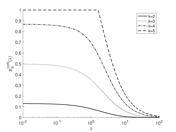
Figure 2. Mean-field approximation: $p_{c}$ as a function of $\lambda$ for $k=2,\ldots,5$, that is, the numerical solution of $\bar{f}_{k}(x)=x$.

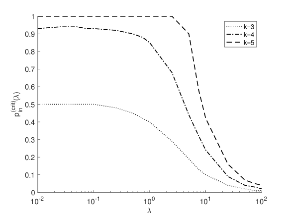
Figure 3. Real process: numerical values for $p^{(crit)}_{in}(\lambda)$ as functions of $\lambda$ for $k=3,\ldots,5$ with $N=100$. Notice that here $p^{(crit)}_{in}(\lambda)$ is rather the threshold where the evolution of the density changes from decreasing to increasing. For more details about simulations see Appendix.

6. Discussion and Conclusions

In this work we introduced the random graph model $G_{\mathbb{Z}^{2}_{N},p_{d}}$. We derived bounds on the diameter of this graph and described its degree distribution. We studied the activation processes on $G_{\mathbb{Z}^{2}_{N},p_{d}}$ and approximated the evolution of the density in the real model with critical values in mean-field. Specifically, we derived conditions for phase transitions as a function of initialization probability $p$ and long edge parameter $\lambda$. The dependence of $p_{c}$ on $\lambda$ in the mean field model and numerical values for $p^{(crit)}_{in}(\lambda)$ in the real model (if exist) are shown on Figures 3, 3, respectively. It seems that $p_{c}$ approximates $p^{(crit)}_{in}(\lambda)$ well.

The model introduced in this paper is motivated by the structure and operation of the neuropil, the densely connected neural tissue of the cortex [18, 23]. The human brain has about $10^{11}$ neurons. Typically, a neuron has several thousands of connections to other neurons through synapses, thus the human brain has $\sim 10^{15}$ synaptic connections. Most of the connections are short and limited to the neuron’s direct neighborhood (in some metric), forming the so-called the dendritic arbor. In addition, the neurons have a few long connections (axons), which extend further away from their cell body. In general, there are several thousands short connections in the dendritic arbor for a few distant connections represented by long axons. We use $G_{\mathbb{Z}^{2}_{N},p_{d}}$ to model the combined effect of mostly short connections and a few long connections. It is much more likely to have in brains shorter connections than longer ones, which is a fact captured in the definition of $p_{d}$, as $p_{d}$ is decreasing in the graph distance $d$.

There are two types of neurons in the brain, namely excitatory and inhibitory ones. The type of a neuron describes the function of the neuron in the brain. Excitatory (inhibitory) neurons excite (inhibit) the neurons to which they are connected. It is known that there are much more excitatory neurons than inhibitory neurons in the cortex; the ratio of inhibitory to excitatory neurons is typically $1/4$ [18]. Based on neuroscience studies, it is expected that pure excitatory populations can maintain non-zero background activation level, while interacting excitatory and inhibitory populations are able to produce limit cycle oscillations [22].

This paper focuses on conditions required to sustain non-zero activity level in pure excitatory networks, but the model can be generalized to include two types of vertices [24]. Here we briefly outline the proposed approach. The type of a vertex is either excitatory ($E$) or inhibitory ($I$). Let $A_{E}(t)$ and $A_{I}(t)$ be the sets of active vertices of type $E$ and $I$ at time $t$, respectively. The total number of active vertices is given by $A(t)=A_{E}(t)\cup A_{I}(t)$. Using the potential function defined in Section 3, we can rewrite $A_{i}(t)=\{v\in V(G_{\mathbb{Z}^{2}_{N},p_{d}})\bigm{|}\chi_{v}(t)=1\ \&~{}v\text{ is of }\text{ type}~{}i\}$, where $i\in\{E,I\}$. Each vertex may change its activity based on the states of its neighbors. We define the modified $k$-threshold rule for two types of vertices as follows. For a vertex $v$ of type $E$, the evolution rule is

(6.1) $$\chi_{v}(t+1)=\mathbbm{1}\left(\sum_{u\in N^{E}(v)}{\chi_{u}(t)}-\sum_{u\in N^{I}(v)}{\chi_{u}(t)}\geq k\right),$$

where $N^{E}(v)$ and $N^{I}(v)$ denote the subsets of vertices in the closed neighborhood of the vertex $v$, of type $E$ and $I$, respectively. For a vertex $v$ of type $I$, the following rule holds:

(6.2) $$\chi_{v}(t+1)=\mathbbm{1}\left(\sum_{u\in N^{E}(v)}{\chi_{u}(t)}+\sum_{u\in N^{I}(v)}{\chi_{u}(t)}\geq k\right)=\mathbbm{1}\left(\sum_{u\in N(v)}{\chi_{u}(t)}\geq k\right),$$

where $N(v)=N^{E}(v)\cup N^{I}(v)$ is the closed neighborhood of vertex $v$. Notice, that vertices of type $E$ and $I$ influence each other differently.

Open problems concerning the properties of $G_{\mathbb{Z}^{2}_{N},p_{d}}$ and the activation process on the graph include: What is the number of small cycles? What is the clustering coefficient? Does a unique limit density defined in Conjectures 1, 2 and 3 exist? Additional open questions include the generalization of these results for other lattice types and higher dimensions.

Acknowledgement.

We are grateful to the unknown referee whose important suggestions led to additional results and improved the presentation of this paper. Figures 1 and 3 are based on simulations that were done by Gabriel P. Andrade.

7. Appendix.

7.1. The second derivative of $\log(P_{k}(x))$

(7.1) $$\left(\log(P_{2}(x))\right)^{\prime\prime}=\frac{-5(\lambda^{4}(1-x)^{4}+16\lambda^{3}(1-x)^{3}+96\lambda^{2}(1-x)^{2}+240\lambda(1-x)+240)}{(1-x)^{2}(\lambda^{2}(1-x)^{2}+10\lambda(1-x)+20)^{2}},$$

(7.2) $$\left(\log(P_{3}(x))\right)^{\prime\prime}=-5\left[\lambda^{6}(1-x)^{6}+24\lambda^{5}(1-x)^{5}\right.\\ \left.+228\lambda^{4}(1-x)^{4}+1056\lambda^{3}(1-x)^{3}+2520\lambda^{2}(1-x)^{2}+2880\lambda(1-x)+1440)\right]\\ \left((1-x)(\lambda^{3}(1-x)^{3}+15\lambda^{2}(1-x)^{2}+60\lambda(1-x)+60)\right)^{-2},$$

(7.3) $$\left(\log(P_{4}(x))\right)^{\prime\prime}=-5\left[\lambda^{8}(1-x)^{8}+32\lambda^{7}(1-x)^{7}+416\lambda^{6}(1-x)^{6}+2784\lambda^{5}(1-x)^{5}\right.\\ \left.+10320\lambda^{4}(1-x)^{4}+21120\lambda^{3}(1-x)^{3}+23040\lambda^{2}(1-x)^{2}+11520\lambda(1-x)+2880\right]\\ \left((1-x)(\lambda^{4}(1-x)^{4}+20\lambda^{3}(1-x)^{3}+120\lambda^{2}(1-x)^{2}+240\lambda(1-x)+120)\right)^{-2},$$

(7.4) $$\left(\log(P_{5}(x))\right)^{\prime\prime}=-5\lambda^{2}\left[\lambda^{8}(1-x)^{8}+40\lambda^{7}(1-x)^{7}+660\lambda^{6}(1-x)^{6}+5760\lambda^{5}(1-x)^{5}\right.\\ \left.+28800\lambda^{4}(1-x)^{4}+83520\lambda^{3}(1-x)^{3}+136800\lambda^{2}(1-x)^{2}+115200\lambda(1-x)+43200\right]\\ (\lambda^{5}(1-x)^{5}+25\lambda^{4}(1-x)^{4}+200\lambda^{3}(1-x)^{3}+600\lambda^{2}(1-x)^{2}+600\lambda(1-x)+120)^{-2}.$$

Clearly, $\left(\log(P_{i}(x))\right)^{\prime\prime}<0$, for $i=2,3,4,5$, $\lambda>0$, $x\in(0,1)$.

7.2. Description of simulations

Figure 1 and 3 in the main text are based on the simulations of the real process on $G_{\mathbb{Z}^{2}_{N},p_{d}}$ with $N=100$, i.e., $|V(G_{\mathbb{Z}^{2}_{N},p_{d}})|=10000$, that were done as follows. For every value of $\lambda$, 15 graphs were generated, each with different random seed. The process was ran on each graph for all initialization probabilities between 0 and 1 with step 0.01. ”Limiting” densities shown on Figure 1 were obtained under the condition that either the density converges after the first 1000 iterations to 0 or 1, or undergoes repetitions after the first 1000 iterations.

References

- [1] Aizenman, M., Kesten, H., and Newman, C.M, Uniqueness of the infinite cluster and continuity of connectivity functions for short and long range percolation, Commun. Math. Phys., 21, 3801-3813, (1988).
- [2] Aizenman, M., and Lebowitz, J., Metastability effects in bootstrap percolation, J. of Physics A, 21, 3801-3813, (1988).
- [3] Albert, R., and Barabasi, A.-L., Statistical mechanics of complex networks, Rev. Mod. Phys. 74, 47-97, (2002).
- [4] Balister, P., Bollobás, B., and Kozma, R., Large deviations for mean field models of probabilistic cellular automata, Random Structures Algorithms 29 (3), 399-415, (2006).
- [5] Balogh, J., Bollobás, B., Duminil-Copin, H., and Morris, R., The sharp thresholdfor bootstrap percolation in all dimensions, Trans. Amer. Math. Soc. 364 (5), 2667-2701, (2012).
- [6] Barbour, A.D., Holst, L., and Janson, S., Poisson approximation, Clarendon Press, Oxford, (1992).
- [7] Benjamini, I., and Berger, N., The diameter of long-range percolation clusters on finite cycles, Random Structures Algorithms, 19 (2), 102-111, (2001).
- [8] Biskup, M., Chayes, L., and Crawford, N., Mean-field driven first-order phase transitions in systems with long-range interactions, J. of Statistical Physics, 122 (6), 1139-1193, (2006).
- [9] Bollobás, B., and Chung, F. R. K., The diameter of a cycle plus a random matching, SIAM J. Disc. Math., 1 (3), 328-333, (1988).
- [10] Bollobás, B., Janson, S., and Riordan, O., The phase transition in inhomogeneous random graphs, Random Structures Algorithms, 31 (1), 3-122, (2007).
- [11] Cerf, R., Manzo, F., The threshold regime of finite volume bootstrap percolation, Stochastic Proc. Appl., 101, 69-82, (2002).
- [12] Chalupa, J., Leath, P.L., and Reich, G.R., Bootstrap percolation on a Bethe lattice, Journal of Physics C, 12 (1):L31, (1979).
- [13] Chung, F., and Lu, L., The diameter of sparse random graphs, Advances in Applied Mathematics, 26, (4), 256-279, (2001).
- [14] Coker, T., and Gunderson, K., A sharp threshold for a modified bootstrap percolation with recovery, J. Stat. Phys. 157, 531-570, (2014).
- [15] Coppersmith, D., Gamarnik, D., and Sviridenko, M., The diameter of a long-range percolation graph, Random Structures Algorithms, 21, (1), 1-13, (2002).
- [16] Einarsson, H., Lengler, J., Mousset, F., Panagiotouy, K., and Steger, A., Bootstrap percolation with inhibition, arxiv, 2015.
- [17] Erdős, P., and Rényi, A., On the evolution of random graphs, Magyar Tudoamányos Akadémia, Mat. Kut. Int. Közl., 5, 17-61, (1960).
- [18] Freeman, W.J., The physiology of perception, Scientific American, 264, 78-85, (1991).
- [19] Hirsch, M. W., Smale, S., and Devaney, R. L., Differential equations, dynamical systems, and an introduction to chaos. Academic Press, (2012).
- [20] Holroyd, A. E., Sharp metastability threshold for two-dimensional bootstrap percolation, Probability Theory and Related Fields, 125:195-224, (2003).
- [21] Janson, S., Łuczak, T., Turova, T., and Vallier, T., Bootstrap percolation on the random graph , The Annals of Applied Probability, 22 (5), 1989-2047, (2012).
- [22] Kozma, R., and Puljic, M., Random graph theory and neuropercolation for modeling brain oscillations at criticality, Current opinion in neurobiology, 31, 181-188, (2015).
- [23] Kozma, R., Puljic, M., Balister, P., Bollobas, B., Freeman, W.J. Phase transitions in the neuropercolation model of neural populations with mixed local and non-local interactions, Biological Cybernetics, 92 (6), 367-379, (2005).
- [24] Kozma, R., Ruszinkó, M., and Sokolov, Y., Percolation on a power-law-like random graph coupled with a lattice. Part II: The case of two types of nodes, in progress.
- [25] Le Cam, L., An approximation theorem for the Poisson binomial distribution, Pacific Journal of Mathematics, 10, 1181-1197, (1960).
- [26] Newman, M. E. J., and Watts, D. J., Scaling and percolation in the small-world network model, Phys. Rev. E, 60, 7332 - 7342, (1999).
- [27] Schonmann, R.H., On the behaviour of some cellular automata related to bootstrap percolation, Annals of Probability, 20:174-193, (1992).
- [28] Talagrand, M., Mean field models for spin glasses, Vol. 1 2, Springer-Verlag Berlin Heidelberg, (2011).
- [29] Turova, T., and Vallier, T., Bootstrap percolation on a graph with random and local connections., J. Stat. Physics, 160, (5), 1249-1276, (2015).
- [30] van Enter, A.C.D., Proof of Straley’s argument for bootstrap percolation, J. Statist. Phys., 48:943-945, (1987).
- [31] Watts, D. J., and Strogatz, S. H., Collective dynamics of ’small-world’ networks, Nature, 440-442 (1998).