An Algorithm for Online Tensor Prediction

Abstract

We present a new method for online prediction and learning of tensors ($N$-way arrays $N>2$) from sequential measurements. We focus on the specific case of 3-D tensors and exploit a recently developed framework of structured tensor decompositions proposed in [1]. In this framework it is possible to treat 3-D tensors as linear operators and appropriately generalize notions of rank and positive definiteness to tensors in a natural way. Using these notions we propose a generalization of the matrix exponentiated gradient descent algorithm [2] to a tensor exponentiated gradient descent algorithm using an extension of the notion of von-Neumann divergence to tensors. Then following a similar construction as in [3], we exploit this algorithm to propose an online algorithm for learning and prediction of tensors with provable regret guarantees. Simulations results are presented on semi-synthetic data sets of ratings evolving in time under local influence over a social network. The result indicate superior performance compared to other (online) convex tensor completion methods.

I Introduction

The problem addressed by this paper is online prediction (completion) of 3-D arrays $\bm{\mathscr{{M}}}\in\mathbb{R}^{n_{1}\times n_{2}\times n_{3}}$, also referred to as tensors. On each round $t$, the predictor (learner) receives a triplet of indices $(i_{t},j_{t},k_{t})$ and predicts the value of $\bm{\mathscr{{M}}}(i_{t},j_{t},k_{t})$. The learner then suffers a loss according to a convex loss function $l_{t}$, which is also selected adversarially from a class of convex functions with bounded Lipschitz continuity. As is normally done in sequential estimation and learning [4, 5], the goal is to minimize long term regret, i.e. the loss compared to the best possible policy in hindsight, over some class of predictors (we make this precise in Section IV).

Motivated by the success of low-rank heuristic for such problems for the case of 2-D arrays [6, 7, 8, 9], to this end we will chose the comparator class based on the assumption that the best estimator belongs to a tensor with low tensor-rank. In this context we exploit a recently proposed tensor factorization strategy proposed in [10]. In this framework, the low-rank nature of a 3-rd order tensor is captured through a matrix like Singular Value Decomposition (SVD), namely tensor-SVD (t-SVD). Similar to the case of algorithms used for matrix completion assuming that the data is sampled from a low rank matrix, recently similar methods based on the t-SVD have found success in tensor completion from missing entries for video (3D and 4D) [11] and seismic (5D) data [12], and we are motivated by the results reported therein. However unlike the methods considered in these papers that assume a batch setting, in this paper we assume that the data is provided in a sequential or streaming manner and the goal is to minimize the long term (cumulative) prediction error.

There are other approaches for tensor prediction in the batch and adaptive sampling situation using other types of tensor factorizations such as Canonincal-Parafac (CP) and Higher Order Singular Value Decomposition (HOSVD),[13, 14]. In contrast our work considers tensor prediction in an online and non-adaptive setting with performance guarantees. To the best of our knowledge the problem of non-adaptive online learning and prediction of tensors (in particular multidimensional data) has not been explicitly considered so far. In order to put our contributions in perspective we begin by a survey of current frameworks used for modeling and prediction of tensor data.

I-A Relation to existing work

Existing work on tensor completion from limited measurements rely upon treating a tensor as an element of outer product of finite dimensional vector spaces [14]. Within this multilinear algebraic framework, tensor completion strategies under several rank-revealing factorizations namely Canonical/Parafac (CP) and Tucker [15] have been proposed, see [16] for methods based on special cases (namely symmetric tensors) of CP decomposition and [17] for methods based on Tucker and Hierarchical-Tucker decompositions. These methods essentially exploit the low rank matrix structure from various un-foldings and reshaping of the tensor. Put another way these methods assume that when a tensor is seen as an element of outer product of vector spaces, each vector space has low dimension. This fact is also exploited in a number of methods, which essentially work by deriving novel norms serving as a low rank convex surrogate, on the set of matrices obtained by mode unfoldings of a tensor [18]. Adaptive (non-adversarial) sampling and recovery methods have also been proposed [19], which are again based on adaptively learning the vector spaces spanned by the tensor fibers.

In contrast to these multilinear algebraic approaches our approach is linear algebraic and is based on the group theoretic approach of [10, 11]. At a high-level this approach essentially rests on unraveling the complexity of the multidimensional structure by constructing group-rings along the tensor fibers, [20]. In this framework a 3-D tensor can be treated as a linear operator acting on the vector space over these group-rings. A rank revealing factorization of this operator then captures the complexity of the multidimensional data, which in turn is useful for prediction. In this paper we will restrict ourselves to cyclic groups, which can capture periodic patterns in the data.

I-B Organization of the paper

We begin by noting necessary background material and preliminaries in Section II. In Section III we derive notions of von Neumann entropy and divergence for tensors. Then in Section IV we state the problem, outline the main results and derive Online Tensor Exponentiated Gradient (OTEG) descent algorithm. Simulation results on synthetic data sets are presented in Section V-C.

I-C Notation

Matrices will be denoted by upper case bold letters ${\bm{\mathbf{{X}}}}$, vectors by lower case boldface letters $\bm{\mathbf{x}}$ and 3-D arrays or tensors will be denoted by $\bm{\mathscr{{X}}}$. Throughout we will use the following notation for denoting the elements, fibers and slices for the tensors and matrices - for a tensor $\bm{\mathscr{{X}}}^{(i)}$ will denote the $i$-th frontal slice of $\bm{\mathscr{{X}}}$, and $\bm{\mathscr{{X}}}_{ij}$ will denote a tensor fiber (or tube) into the board. We will also use the following convention for denoting the tensor fibers - $\bm{\mathscr{{X}}}(:,:,k)$ denotes the $k$-th frontal face, $\bm{\mathscr{{X}}}(:,j,:)$ denotes the $j$-th lateral slice and $\bm{\mathscr{{X}}}(i,:,:,)$ denotes the $i$-th horizontal slice. Similarly ${\bm{\mathbf{{X}}}}(:,i)$ denotes the $i$-th column of the matrix and so on. For any third order tensor $\bm{\mathscr{{X}}}$, $\widehat{\bm{\mathscr{{X}}}}$ denotes the 3-D tensor of the same size obtained by taking the Fourier transform along the third dimension (also c.f. Algorithm 1 in Section II-B).

II Linear algebra for 3-D tensors

We will now briefly review the linear algebraic concepts first developed in [1] shown to be useful in a variety of applications [21, 11, 12].

II-A t-product: Tensor as a linear operator

Figure 1: 3-D tensors as operators on oriented matrices.

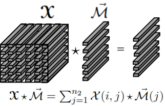
In the framework proposed in [1] a 3-D array is defined as a linear operator using the t-product defining the multiplication action. There are several ways to define the t-product, and we take the development directly from [11]. We begin by viewing a 3-D tensor $\bm{\mathscr{{X}}}\in\mathbb{R}^{n_{1}\times n_{2}\times n_{3}}$ as an $n_{1}\times n_{2}$ matrix (say) $\mathcal{X}$ of tubes (vectors oriented into the board), whose $i,j$-th entry $\mathcal{X}(i,j)=\bm{\mathscr{{X}}}(i,j,:)$. Similarly one can consider a $n_{1}\times 1\times n_{3}$ tensor as a vector of tubes. Such tensors are referred to as oriented matrices, [1] and are denoted by $\vec{\mathcal{M}}$.

Now in order to define the 3-D tensor as a linear operator on the set of oriented matrices $\vec{\mathcal{M}}$ [22], one defines a multiplication operation between two tubes $\vec{\bm{\mathbf{v}}}\in\mathbb{R}^{1\times 1\times n_{3}}$ and $\vec{\bm{\mathbf{u}}}\in\mathbb{R}^{1\times 1\times n_{3}}$ resulting in another tube of same length. Specifically this multiplication operation is given by circular convolution denoted by $\star$. Under this construction, the operation of a tensor $\bm{\mathscr{{X}}}$ on $\vec{\mathcal{M}}\in\mathbb{R}^{n_{2}\times 1\times n_{3}}$ is another oriented matrix of size $n_{1}\times 1\times n_{3}$ whose $i$-th tubal element given by, $\bm{\mathscr{{X}}}\star\vec{\mathcal{M}}=\sum_{j=1}^{n_{2}}\mathcal{X}(i,j)\star\vec{\mathcal{M}}(j)$ as illustrated in Figure 1. Similarly one can extend this definition to define the multiplication of two tensors $\bm{\mathscr{{X}}}$ and $\bm{\mathscr{{Y}}}$ of sizes $n_{1}\times n_{2}\times n_{3}$ and $n_{2}\times k\times n_{3}$ respectively, resulting in a tensor $\bm{\mathscr{{C}}}=\bm{\mathscr{{X}}}\star\bm{\mathscr{{Y}}}$ of size $n_{1}\times k\times n_{3}$. This product between two tensors is referred to as the t-product.

II-B t-SVD

Under the above construction viewing a 3-D tensor as a linear operator over the set of oriented matrices, one can compute a tensor-Singular Value Decomposition (t-SVD) as shown in Figure 2. Since $\star$ is given by the circular convolution the t-SVD can be computed using the Fast Fourier Transform (fft) using Algorithm 1 [1].

Figure 2: t-SVD under the t-product

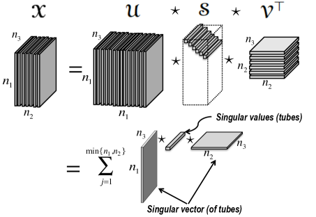
The component tensors $\bm{\mathscr{{U}}}$ and $\bm{\mathscr{{V}}}$ obey the orthogonality conditions $\bm{\mathscr{{U}}}^{\top}\star\bm{\mathscr{{U}}}=\bm{\mathscr{{I}}}$, $\bm{\mathscr{{V}}}^{\top}\star\bm{\mathscr{{V}}}=\bm{\mathscr{{I}}}$ with the following definitions for tensor transpose $(\cdot)^{\top}$ and and identity tensor $\bm{\mathscr{{I}}}$ (of appropriate dimensions).

Definition II.1.

Tensor Transpose. Let $\bm{\mathscr{{X}}}$ be a tensor of size $n_{1}\times n_{2}\times n_{3}$, then $\bm{\mathscr{{X}}}^{\top}$ is the $n_{2}\times n_{1}\times n_{3}$ tensor obtained by transposing each of the frontal slices and then reversing the order of transposed frontal slices $2$ through $n_{3}$.

Definition II.2.

Identity Tensor. The identity tensor $\bm{\mathscr{{I}}}\in\mathbb{R}^{n\times n\times n_{3}}$ is a tensor whose first frontal slice is the $n\times n$ identity matrix and all other frontal slices are zero.

Algorithm 1 tSVD

  Input: $\bm{\mathscr{{X}}}\in\mathbb{R}^{n_{1}\times n_{2}\times n_{3}}$

  Take Fourier transform along the 3 dimension

  ${\widehat{\bm{\mathscr{{X}}}}}\leftarrow\mbox{\tt fft}(\bm{\mathscr{{X}}},[\hskip 2.84526pt],3)$;

  for $i=1\hskip 5.69054pt\rm{to}\hskip 5.69054ptn_{3}$ do

     $[\hat{{\bm{\mathbf{{U}}}}},\hat{{\bm{\mathbf{{S}}}}},\hat{{\bm{\mathbf{{V}}}}}]={\tt SVD}(\widehat{\bm{\mathscr{{X}}}}^{(i)})$

     ${\widehat{\bm{\mathscr{{U}}}}}^{(i)}=\hat{{\bm{\mathbf{{U}}}}};{\widehat{\bm{\mathscr{{S}}}}}^{(i)}=\hat{{\bm{\mathbf{{S}}}}}$; $\widehat{\bm{\mathscr{{V}}}}^{(i)}=\hat{{\bm{\mathbf{{V}}}}};$

  end for

  Take inverse Fast Fourier Transform ${\tt ifft}$ along the 3 dimension for each of the component tensors

  $\bm{\mathscr{{U}}}\leftarrow\mbox{\tt ifft}(\widehat{\bm{\mathscr{{U}}}},[\hskip 2.84526pt],3);$ $\bm{\mathscr{{S}}}\leftarrow\mbox{\tt ifft}(\widehat{\bm{\mathscr{{S}}}},[\hskip 2.84526pt],3);$

  $\bm{\mathscr{{V}}}\leftarrow\mbox{\tt ifft}(\widehat{\bm{\mathscr{{V}}}},[\hskip 2.84526pt],3)$;

II-B1 Alegbraic Complexity measures from t-SVD

Under the t-SVD, it is clear that [10] if the number of non-zero singular tubes in $\bm{\mathscr{{S}}}$ is $r$, there exist a set of oriented matrices $\bm{\mathscr{{X}}}(:,j^{\prime},:),j^{\prime}\in J:|J|=r$ such that each $\bm{\mathscr{{X}}}(:,i,:)$ can be written as

$$\bm{\mathscr{{X}}}(:,j,:)=\sum_{j^{\prime}\in J}\bm{\mathscr{{X}}}(:,j^{\prime},:)\star\vec{\bm{\mathbf{\ell}}}_{j\prime}^{j}.$$

From t-SVD one can readily extract several notions of complexity of the data in terms of “rank”. The notion of multi-rank was proposed in [10] using the Fourier Domain representation of t-SVD as the vector of ranks of the slices $\widehat{\bm{\mathscr{{X}}}}(:,:,i),i=1,2,...,n_{3}$. The $\ell_{1}$ norm of the multi-rank can be taken to be a measure of the complexity of the data. On the other hand, similar to matrix completion, where the nuclear norm is used as a useful convex surrogate to low rank, one employs a similar measure form t-SVD known as Tensor Nuclear Norm (TNN) [11]. TNN, denote by denoted $\|\bm{\mathscr{{X}}}\|_{TNN}$ is the sum of nuclear norms of the slices $\widehat{\bm{\mathscr{{X}}}}({:,:,i})$. In this paper we will derive complexity measures which are related to TNN and use them to define the class of predictors against which, we will find bounds on the regret.

III Positive-Definite Tensors and von Neumann Entropy

Based on the t-SVD we define the notion of positive definite tensors.

Definition III.1.

Positive Definite Tensor: A tensor is positive definite under the t-product if each frontal slice $\widehat{\bm{\mathscr{{X}}}}^{(i)}$ in the transformed domain is positive definite.

Similar definition applies to a symmetric positive definite tensors. In the following we will denote by $\mathrsfs{S}^{N\times N\times d}_{++}$ the set of all symmetric positive definite tensors.

Definition III.2 (Trace of a Tensor).

The trace of the tensor $\bm{\mathscr{{X}}}\in\mathbb{R}^{n_{1}\times n_{2}\times n_{3}}$ is defined as the trace of $\mbox{\tt blkdiag}(\widehat{\bm{\mathscr{{X}}}})$ where $\mbox{\tt blkdiag}(\widehat{\bm{\mathscr{{X}}}})$ is a block diagonal matrix whose diagonal blocks are given by $\widehat{\bm{\mathscr{{X}}}}^{(i)}$.

Let $\mbox{\tt reshapeT}(\mbox{\tt blkdiag}(\widehat{\bm{\mathscr{{X}}}}))$ denote the reshaping of $\mbox{\tt blkdiag}(\widehat{\bm{\mathscr{{X}}}})$ back to the tensor $\widehat{\bm{\mathscr{{X}}}}$ and $\bm{\mathscr{{X}}}^{k}=\underset{k\,\,\mbox{times}}{\underbrace{\bm{\mathscr{{X}}}\star\bm{\mathscr{{X}}}\star\ldots\star\bm{\mathscr{{X}}}}}$ for a positive integer $k$ and and $\bm{\mathscr{{X}}}^{0}=\bm{\mathscr{{I}}}$.

Definition III.3.

Let $\bm{\mathscr{{X}}}\in\mathrsfs{S}^{N\times N\times d}_{++}$. Then, under the t-product, we define the tensor exponential as $\exp(\bm{\mathscr{{X}}})\triangleq\sum_{k=0}^{\infty}\frac{1}{k!}\bm{\mathscr{{X}}}^{k}$.

By a straightforward calculation it can be shown that

$$\exp\bm{\mathscr{{X}}}=\mbox{\tt ifft}\left(\mbox{\tt reshapeT}\left(\exp\left(\mbox{\tt blkdiag}(\widehat{\bm{\mathscr{{X}}}})\right)\right),[\,],3\right),$$

where the matrix exponential is defined in the usual way.

Definition III.4 (Logarithm of a Tensor).

For $\bm{\mathscr{{X}}}\in\mathrsfs{S}^{N\times N\times d}_{++}$, in line with the definition of tensor exponential, we define the logarithm of a tensor $\bm{\mathscr{{X}}}$ as

$$\log\bm{\mathscr{{X}}}\triangleq\mbox{\tt ifft}\left(\mbox{\tt reshapeT}\left(\log\left(\mbox{\tt blkdiag}(\widehat{\bm{\mathscr{{X}}}})\right)\right),[\,],3\right),$$

where the matrix logarithm is defined in the usual way.

III-A Von-Neumann Entropy for Tensors

We begin by extending the notion of Von-Neumann entropy for PD symmetric matrices [23] to PD tensors via the following.

Definition III.5.

The von-Neumann entropy of a tensor $\in\mathrsfs{S}^{N\times N\times d}_{++}$ is defined as

$${\cal{H}}(\bm{\mathscr{{W}}})$$

$$\triangleq\mathrm{Tr}\left(\mbox{\tt blkdiag}(\widehat{\bm{\mathscr{{W}}}})\log(\mbox{\tt blkdiag}(\widehat{\bm{\mathscr{{W}}}}))-\mbox{\tt blkdiag}(\widehat{\bm{\mathscr{{W}}}})\right)$$

$$=\sum_{k=1}^{d}\mathrm{Tr}\left(\widehat{\bm{\mathscr{{W}}}}^{(k)}\log(\widehat{\bm{\mathscr{{W}}}}^{(k)})-\widehat{\bm{\mathscr{{W}}}}^{(k)}\right)$$

$$\triangleq\hat{{\cal H}}(\widehat{\bm{\mathscr{{W}}}})$$

Note that by definition of the tensor trace, we can write, ${\cal{H}}(\bm{\mathscr{{W}}})=\mathrm{Tr}(\bm{\mathscr{{W}}}\star\log\bm{\mathscr{{W}}}-\bm{\mathscr{{W}}})$. Let us define an inner product on the space of real tensors via the t-product.

Definition III.6 (Inner product of two tensors).

The inner product between two $n_{1}\times n_{2}\times n_{3}$ tensors $\bm{\mathscr{{X}}},\bm{\mathscr{{Y}}}$ is defined as

$$\langle\bm{\mathscr{{X}}},\bm{\mathscr{{Y}}}\rangle=\mathrm{Tr}(\bm{\mathscr{{X}}}\star\bm{\mathscr{{Y}}}^{\top})=\mathrm{Tr}(\mbox{\tt blkdiag}(\widehat{\bm{\mathscr{{X}}}})\mbox{\tt blkdiag}(\widehat{\bm{\mathscr{{Y}}}})^{\dagger})\,\,,$$

where $\dagger$ denotes Hermitian transpose.

We now derive the von-Neumann divergence $\Delta_{H}(\bm{\mathscr{{W}}}^{\prime},\bm{\mathscr{{W}}})$ between tensors $\bm{\mathscr{{W}}},\bm{\mathscr{{W}}}^{\prime}\in\mathrsfs{S}^{N\times N\times d}_{++}$. Note that under the t-product we have,

$$\Delta_{H}(\bm{\mathscr{{W}}}^{\prime},\bm{\mathscr{{W}}})$$

$$={\cal H}(\bm{\mathscr{{W}}}^{\prime})-{\cal H}(\bm{\mathscr{{W}}})-\mathrm{Tr}\left((\bm{\mathscr{{W}}}^{\prime}-\bm{\mathscr{{W}}})\star(\nabla_{\bm{\mathscr{{W}}}}{\cal H}(\bm{\mathscr{{W}}}))^{\top}\right)$$

$$\stackrel{{\scriptstyle(a)}}{{=}}{\cal H}(\bm{\mathscr{{W}}}^{\prime})-{\cal H}(\bm{\mathscr{{W}}})-\mathrm{Tr}\left((\bm{\mathscr{{W}}}^{\prime}-\bm{\mathscr{{W}}})\star(\log\bm{\mathscr{{W}}})^{\top}\right)$$

$$=\hat{{\cal H}}(\widehat{\bm{\mathscr{{W}}}}^{\prime})-\hat{{\cal H}}(\widehat{\bm{\mathscr{{W}}}})$$

$$\hskip 19.91692pt-\mathrm{Tr}\left(\mbox{\tt blkdiag}(\widehat{\bm{\mathscr{{W}}}}^{\prime}-\widehat{\bm{\mathscr{{W}}}})[\log(\mbox{\tt blkdiag}(\widehat{\bm{\mathscr{{W}}}}))]^{\dagger}\right)$$

where (a) follows from the Lemma VII.1 in the Appendix and the fact that

$$\nabla_{\widehat{\bm{\mathscr{{W}}}}}\hat{{\cal H}}(\widehat{\bm{\mathscr{{W}}}})=\mbox{\tt reshapeT}(\log(\mbox{\tt blkdiag}(\widehat{\bm{\mathscr{{W}}}})))\,\,,$$

see [24],[25].

IV Online prediction for tensors: Problem set-up and main results

For the problem of online tensor prediction, the complexity structure that we impose on the data tensor stems from the $(\beta,\tau)$ decomposability construction found in [3] to express ordinary matrices in a positive definite form. Let’s begin by defining the original matrix decomposition therein.

Definition IV.1.

Let ${\bm{\mathbf{{A}}}}\in\mathbb{R}^{m\times n}$ be any real matrix. The symmetrization of ${\bm{\mathbf{{A}}}}$, $\mathrm{sym}({\bm{\mathbf{{A}}}})$, is defined as

$$\mathrm{sym}({\bm{\mathbf{{A}}}})=\begin{pmatrix}0&{\bm{\mathbf{{A}}}}\\ {\bm{\mathbf{{A}}}}^{T}&0\end{pmatrix}$$

Definition IV.2.

Let $p$ be the dimension of $\mathrm{sym}({\bm{\mathbf{{A}}}})$. Then ${\bm{\mathbf{{A}}}}$ is $(\beta,\tau)$-decomposable for real numbers $\beta$ and $\tau$ if there exist positive-semidefinite matrices ${\bm{\mathbf{{P}}}},{\bm{\mathbf{{N}}}}\in\mathrsfs{S}^{p\times p}_{+}$ such that

(1)

$\mathrm{sym}({\bm{\mathbf{{A}}}})={\bm{\mathbf{{P}}}}-{\bm{\mathbf{{N}}}}$

(2)

$\forall i,{\bm{\mathbf{{P}}}}(i,i),{\bm{\mathbf{{N}}}}(i,i)\leq\beta$

(3)

$\mathrm{Tr}({\bm{\mathbf{{P}}}})+\mathrm{Tr}({\bm{\mathbf{{N}}}})\leq\tau$

It turns out the notion of $(\beta,\tau)$-decomposability is tightly related to the max norm and nuclear norm of ${\bm{\mathbf{{A}}}}$, making it simple to find suitable decomposition parameters for any class of matrices. More precisely, the least possible $\tau$ used to decompose a matrix ${\bm{\mathbf{{A}}}}$ is equal to $2\|{\bm{\mathbf{{A}}}}\|_{*}$, and the least possible $\beta$ is $\frac{1}{2}||{\bm{\mathbf{{A}}}}||_{\infty}$ [3], where $||\cdot||_{*}$ and $||\cdot||_{\infty}$ denote the matrix nuclear norm and $\ell_{\infty}$-norm.

We will now extend this notion to tensors.

IV-A The class of $(\bm{\mathbf{\beta}},\bm{\mathbf{\tau}})$-decomposable tensors

Definition IV.3.

Let $\bm{\mathscr{{A}}}\in\mathbb{R}^{m\times n\times d}$ be any tensor. We say that $\bm{\mathscr{{A}}}$ is $(\bm{\mathbf{\beta}},\bm{\mathbf{\tau}})$-decomposable for $\bm{\mathbf{\beta}}$,$\bm{\mathbf{\tau}}\in\mathbb{R}^{d}$, if $\forall k\in[d]$, $\widehat{{\bm{\mathbf{{A}}}}}^{(k)}$ is $(\beta(k),\tau(k))$ decomposable. Additionally, we say a set $\mathrsfs{S}\in\mathbb{R}^{m\times n\times d}$ is $(\bm{\mathbf{\beta}},\bm{\mathbf{\tau}})$-decomposable if each tensor in $\mathrsfs{S}$ is $(\bm{\mathbf{\beta}},\bm{\mathbf{\tau}})$-decomposable.

Note the distinction between the tensor and matrix case: decomposability of a tensor is determined in the Fourier domain. Indeed, $(\bm{\mathbf{\beta}},\bm{\mathbf{\tau}})$-decomposability implies disjoint, face-wise complexity restrictions on the Fourier tensor, which in turn captures the number of non zero singular tubes in the t-SVD of the tensor.

We now state the central problem addressed by this paper in the box below. The goal of Online Tensor Prediction is to minimize regret, which is defined as

$$\mathrm{Regret}\triangleq\sum_{t=1}^{T}l_{t}(\bm{\mathscr{{A}}}_{t}(i_{t},j_{t},k_{t}))-\arg\min_{\bm{\mathscr{{U}}}\in\mathrsfs{S}}\sum_{t=1}^{T}l_{t}(\bm{\mathscr{{U}}}(i_{t},j_{t},k_{t}))$$

Online Tensor Prediction

parameters: $\bm{\mathbf{\beta}}\succeq 0$ with $||\bm{\mathbf{\beta}}||_{1}\geq 1$, $\bm{\mathbf{\tau}}\succeq 0$, $G\geq 0$, $m$, $n$, $d$

input: A $(\bm{\mathbf{\beta}},\bm{\mathbf{\tau}})$-decomposable set $\mathrsfs{S}\subseteq[-1,1]^{m\times n\times d}$

for $t=1,2,3,...T$

adversary supplies indices $(i_{t},j_{t},k_{t})\in[m]\times[n]\times[d]$

learner predicts $p_{t}=\bm{\mathscr{{A}}}_{t}(i_{t},j_{t},k_{t})$ from a maintained tensor $\bm{\mathscr{{A}}}_{t}\in\mathrsfs{S}$

adversary supplies a convex, $G$-Lipschitz function $l_{t}:[-1,1]\rightarrow\mathbb{R}$

learner suffers loss $l_{t}(p_{t})$

end for

Given the set up, our main result is summarized by the following theorem.

Theorem IV.1.

[Main Result] There exists an algorithm for Online Tensor Prediction with regret bounded by

$$Regret\leq 2G\sqrt{\log(2p)T(\sum_{k=1}^{d}\tau(k))(\sum_{k=1}^{d}\beta(k))}$$

where $p$ is the dimension of each $\mathrm{sym}(\widehat{{\bm{\mathbf{{A}}}}}^{(k)})$.

Proof outline: The algorithm is given in Section IV-C. For this algorithm We find the regret bound for our algorithm by linearly approximating the loss functions and applying a linear regret bound to obtain Theorem IV.1. To find the linear bound, we rely on the $(\bm{\mathbf{\beta}},\bm{\mathbf{\tau}})$-decomposability of the learning set to transfer the problem to a positive-definite domain, allowing us to use the Tensor Exponentiated Gradient algorithm, which is derived below. The complete proof can be found in the Appendix. Several important ingredients in the proof rely on some key results on gradient calculus in complex Hilbert spaces.

IV-B Tensor Exponentiated Gradient (TEG) Descent algorithm

We first derive an online algorithm for learning of symmetric PD tensors.

TEG set-up: On each round $t$, we are given an instance tensor $\bm{\mathscr{{X}}}_{t}\in\mathbb{R}^{N\times N\times d}$, the learner predicts the tensor $\bm{\mathscr{{W}}}_{t}$ from a convex set $\mathrsfs{W}\subseteq\mathrsfs{S}^{N\times N\times d}_{++}$, receives a convex loss function $L_{t}:\mathrsfs{W}\rightarrow\mathbb{R}$, and suffers the loss $L_{t}(\bm{\mathscr{{W}}}_{t})$.

For all $t$, we assume that the gradient $\nabla_{\bm{\mathscr{{W}}}}L_{t}$, which is a tensor, is well defined and face-wise symmetric. In addition we assume there exists a function $\widehat{L}_{t}(\widehat{\bm{\mathscr{{W}}}})$ which is convex in $\widehat{\bm{\mathscr{{W}}}}$ with $L_{t}(\bm{\mathscr{{W}}})=\widehat{L}_{t}(\widehat{\bm{\mathscr{{W}}}})$. Clearly, $\widehat{L}_{t}(\widehat{\bm{\mathscr{{W}}}})=L_{t}(\mbox{\tt ifft}(\widehat{\bm{\mathscr{{W}}}},[\,],3))$.

Following [2] we now derive the Tensor Exponentiated Gradient update, which is equivalent to a standard Matrix Exponentiated Gradient with block-diagonal matrices –

$$\bm{\mathscr{{W}}}_{t+1} =\arg\min_{\bm{\mathscr{{W}}}\in\mathrsfs{W}}\Delta_{H}(\bm{\mathscr{{W}}},\bm{\mathscr{{W}}}_{t})+\eta\langle\bm{\mathscr{{W}}},\nabla_{\bm{\mathscr{{W}}}}L_{t}(\bm{\mathscr{{W}}}_{t})\rangle$$

where $\eta$ is the learning rate. Equivalently in the Fourier domain we have,

$$\widehat{\bm{\mathscr{{W}}}}_{t+1}= \arg\min_{\widehat{\bm{\mathscr{{W}}}}\in\widehat{\mathrsfs{W}}}\Delta_{\widehat{H}}(\widehat{\bm{\mathscr{{W}}}},\widehat{\bm{\mathscr{{W}}}}_{t})$$

$$\hskip 2.84526pt+\eta\mathrm{Tr}\left(\mbox{\tt blkdiag}(\widehat{\bm{\mathscr{{W}}}})\,[\mbox{\tt blkdiag}(\nabla_{\widehat{\bm{\mathscr{{W}}}}}\widehat{L}_{t}(\widehat{\bm{\mathscr{{W}}}}_{t}))]^{\dagger}\right),$$ (1)

where $\widehat{\mathrsfs{W}}$ denotes the set of tensors obtained by taking the Fourier transform of each tensor in $\mathrsfs{W}$. From [2] and [3], we know that the closed form solution to optimization problem in Equation (IV-B) is given by a projected exponentiated gradient descent of Equation (2).

$$\widehat{\bm{\mathscr{{W}}}}_{t+1}=\arg\min_{\widehat{\bm{\mathscr{{W}}}}\in\widehat{\mathrsfs{W}}}\Delta_{\widehat{H}}\left(\widehat{\bm{\mathscr{{W}}}},\mbox{\tt reshapeT}\left(\exp\left(\log(\mbox{\tt blkdiag}(\widehat{\bm{\mathscr{{W}}}}_{t}))-\mbox{\tt blkdiag}\left(\eta\nabla_{\widehat{\bm{\mathscr{{W}}}}}\widehat{L}_{t}(\widehat{\bm{\mathscr{{W}}}}_{t})\right)\right)\right)\right)$$ (2)

Recalling that $\bm{\mathscr{{W}}}_{t}=\mbox{\tt ifft}(\widehat{\bm{\mathscr{{W}}}}_{t},[\,],3)$, we obtain the Tensor Exponentiated Gradient algorithm for online learning of symmetric PD tensors. Note that the optimization in the equation above can be parallelized, since $\exp$ and $\log$ of a block-diagonal matrix are computed block-by-block.

IV-C An Algorithm for Online Tensor Prediction

We begin with a simple construction that lets us represent a $(\bm{\mathbf{\beta}},\bm{\mathbf{\tau}})$-decomposable tensor as a positive-definite tensor. Let $\mathrsfs{S}\subseteq[-1,1]^{m\times n\times d}$ be a $(\bm{\mathbf{\beta}},\bm{\mathbf{\tau}})$-decomposable set. For $\bm{\mathscr{{A}}}\in\mathrsfs{S}$, let $\widehat{\bm{\mathscr{{P}}}}$,$\widehat{\bm{\mathscr{{N}}}}\in\mathrsfs{S}^{p\times p\times d}_{+}$ be the Fourier tensors such that $\mathrm{sym}(\widehat{{\bm{\mathbf{{A}}}}}^{(k)})=\widehat{{\bm{\mathbf{{P}}}}}^{(k)}-\widehat{{\bm{\mathbf{{N}}}}}^{(k)}$. We define $\widehat{\phi}:\mathrsfs{S}\to\mathbb{C}^{2p\times 2p\times d}$ face-wise as

$$\widehat{\phi}(\bm{\mathscr{{A}}})^{(k)}=\begin{pmatrix}\widehat{{\bm{\mathbf{{P}}}}}^{(k)}&0\\ 0&\widehat{{\bm{\mathbf{{N}}}}}^{(k)}\end{pmatrix}$$

The set of all such $\widehat{\phi}$ constructions over the learning set $\mathrsfs{S}$ will be contained in the convex set $\widehat{\mathrsfs{W}}$, defined by Equation (3).

$$\widehat{\mathrsfs{W}}= \left\{\ \widehat{\bm{\mathscr{{W}}}}\in\mathbb{C}^{2p\times 2p\times d}:\forall k,\widehat{{\bm{\mathbf{{W}}}}}^{(k)}\succeq 0,\forall k\forall i,\widehat{{\bm{\mathbf{{W}}}}}^{(k)}(i,i)\leq\beta(k)\right.$$

$$\ \ \left.\forall k,\mathrm{Tr}(\widehat{{\bm{\mathbf{{W}}}}}^{(k)})\leq\tau(k),\,\,\forall(i,j,k)\in[m]\times[n]\times[d]:P_{\widehat{\bm{\mathscr{{W}}}}}(i,j,k)\in[-1,1]\right\}$$ (3)

Algorithm 2 Tensor Exponentiated Gradient for Online Tensor Prediction (OTEG)

  input: $m$,$n$,$d$,$G$,$\bm{\mathbf{\beta}}$, $\bm{\mathbf{\tau}}$ set: $p=m+n$, $N=2p$, $\widehat{\mathrsfs{W}}$ as in (3), $\forall k:\gamma(k)=4G^{2}$ $\eta=\sqrt{\frac{\log N\sum_{k=1}^{d}\tau(k)}{T\sum_{k=1}^{d}\gamma(k)\beta(k)}}$ initialize: $\forall k:\widehat{{\bm{\mathbf{{W}}}}}_{1}^{(k)}=\frac{\tau(k)}{N}{\bm{\mathbf{{I}}}}$

  for $t=1,2,3,...$ do

     Receive triplet of indices $(i_{t},j_{t},k_{t})\in[m]\times[n]\times[d]$ Predict $p_{t}=P_{\widehat{\bm{\mathscr{{W}}}}}(i_{t},j_{t},k_{t})$ Receive $G$-Lipschitz, convex loss function      $l_{t}:[-1,1]\rightarrow\mathbb{R}$ and suffer loss $l_{t}(p_{t})$ Calculate the subderivative $g$ of $l_{t}$ at $p_{t}$ Construct loss tensor $\widehat{\bm{\mathscr{{L}}}}_{t}=\nabla_{\widehat{\bm{\mathscr{{W}}}}}\widehat{L}_{t}(\widehat{\bm{\mathscr{{W}}}}_{t})$Update $\widehat{\bm{\mathscr{{W}}}}_{t+1}$ by solving (IV-B)

  end for

Where $P_{\widehat{\bm{\mathscr{{W}}}}}(i,j,k)=[\mbox{\tt ifft}(\widehat{\bm{\mathscr{{P}}}}-\widehat{\bm{\mathscr{{N}}}})](i,j+m,k)\triangleq p_{t}$ is the so-called “prediction” operator, which extracts $\bm{\mathscr{{A}}}_{t}(i,j,k)$ from the its positive-definite embedding $\widehat{\phi}(\bm{\mathscr{{A}}}_{t})=\bm{\mathscr{{W}}}_{t}$. In our case, $\bm{\mathscr{{X}}}_{t}$ is a tensor that encodes the indices $(i_{t},j_{t},k_{t})$, and we restrict our loss functions to the form $L_{t}(\bm{\mathscr{{W}}}_{t})=l_{t}(p_{t})$. Note that since $\widehat{\mathrsfs{W}}$ is composed of Fourier-domain tensors, the tensor entries will be complex in general, but with real face-wise diagonal entries and trace since the frontal faces are Hermitian.

In order to apply Tensor Exponentiated Gradient, we must compute $\nabla_{\widehat{\bm{\mathscr{{W}}}}}l_{t}(P_{\widehat{\bm{\mathscr{{W}}}}_{t}}(i_{t},j_{t},k_{t}))$, the gradient of the current loss with respect to $\widehat{\bm{\mathscr{{W}}}}$. We have

$$\nabla_{\widehat{\bm{\mathscr{{W}}}}}l_{t}(P_{\widehat{\bm{\mathscr{{W}}}}_{t}}(i_{t},j_{t},k_{t}))$$

$$\stackrel{{\scriptstyle(a)}}{{=}}\nabla_{p}l_{t}(p_{t})\nabla_{\widehat{\bm{\mathscr{{W}}}}}P_{\widehat{\bm{\mathscr{{W}}}}_{t}}(i_{t},j_{t},k_{t})$$

$$\stackrel{{\scriptstyle(b)}}{{=}}g\nabla_{\widehat{\bm{\mathscr{{W}}}}}P_{\widehat{\bm{\mathscr{{W}}}}_{t}}(i_{t},j_{t},k_{t})$$

where $(a)$ follows from the chain rule, and $(b)$ defines $g=\nabla_{p}l_{t}(p_{t})$.

We see the gradient is split into two components: the “time domain gradient” ($g$), and the “Fourier domain gradient” ($\nabla_{\widehat{\bm{\mathscr{{W}}}}}P_{\widehat{\bm{\mathscr{{W}}}}_{t}}(i_{t},j_{t},k_{t})$), which will be a complex gradient of a real-valued function (see [25]).

$$\widehat{\bm{\mathscr{{L}}}}_{t}(i,j,:)=\begin{cases}g{\bm{\mathbf{{F}}}}(:,k)&\mathrm{if}\ (i,j)=(i_{t},j_{t}+m)\\ -g{\bm{\mathbf{{F}}}}(:,k)&\mathrm{if}\ (i,j)=(i_{t}+p,j_{t}+m+p)\\ g\overline{{\bm{\mathbf{{F}}}}}(:,k)&\mathrm{if}\ (i,j)=(j_{t}+m,i_{t})\\ -g\overline{{\bm{\mathbf{{F}}}}}(:,k)&\mathrm{if}\ (i,j)=(j_{t}+m+p,i_{t}+p)\\ 0&\mathrm{otherwise}\end{cases}$$

By straightforward calculation we find an explicit expression of the gradient (LHS), which is built by arranging copies of one column of the DFT matrix ${\bm{\mathbf{{F}}}}$ and its complex conjugate along tubes in the third dimension. Note that each $\widehat{{\bm{\mathbf{{L}}}}}_{t}^{(k)}$ is Hermitian, as required by the Tensor Exponentiated Gradient update, and that $(\widehat{{\bm{\mathbf{{L}}}}}_{t}^{(k)})^{2}$ is a matrix with four copies of $g^{2}$. In fact, since $g\leq G$, we can now write a $\bm{\mathbf{\gamma}}$ constraint for $\widehat{\bm{\mathscr{{L}}}}_{t}$ – $\forall k,\gamma(k)=4G^{2}$.

Based on this development our algorithm for Online Tensor Prediction is given in Algorithm 2. For convenience, we assume that the tensor with faces $\widehat{{\bm{\mathbf{{W}}}}}^{(k)}=\frac{\tau(k)}{N}{\bm{\mathbf{{I}}}}$ is in $\widehat{\mathrsfs{W}}$.

V Experimental validation

V-A Generation of semi-synthetic temporal rating dataset

For experimentation we generated coupled-time dynamics in recommendation systems with social network interaction. Specifically, we generated a semi-synthetic data set of user ratings evolving over time in the following manner. True rating data set was taken from the Movie Lens [26] movie rating observation data and then truncated to only 150 users and 100 movies in order to manage the size of the simulation. In this data set, every user had rated at least 20 movies, but not all 100, so we used a low rank completion method [9] to complete the initial rating matrix. We then mapped the users to a social network taken from the Stanford Network Analysis Project (SNAP) [27]. Our network was a subset of an undirected graph with 1034 nodes and 88234 edges and an average clustering coefficient of 0.6055. We simply used the first 150 nodes in the network to represent our users. Then we took the initial complete rating matrix and evolved the ratings of the users by using the following two influence models as dictated by the social network.

• Dataset A: Evolution with neighborhood influence- For this data set we used the following evolution model for the ratings tensor $\bm{\mathscr{{M}}}$. At each time epoch $s$ the users update their ratings according to,

  $$\bm{\mathscr{{M}}}(u,m,s)=a(s)\,\mbox{Neighbor}\,\,+\,\,b(s)\,\mbox{Self}$$ (4)

  where,

  $$\mbox{Neighbor}=\frac{\sum_{u^{\prime}\in{\cal N}(u)}\bm{\mathscr{{M}}}(u^{\prime},m,s-1)}{|{\cal N}(u)|}$$ (5)

  $$\mbox{Self}=\frac{\bm{\mathscr{{M}}}(u,m,s-1)+{\tt rand}([1:5])}{2}$$ (6)

  and where ${\cal N}(u)$ denotes the set of neighbors (in the undirected graph) of user $u$ and the function ${\tt rand}([1:5])$ outputs a random rating between 1 and 5. In this evolution $a(s)\in[0,1]$ are random constants and $b(s)=1-a(s)$. The reason for selecting this evolution pattern is based on the following. We know that the new rating should be a combination of neighborhood influence, past opinions (personal rating at previous time), and a random influence or self-innovation. The amount of influence that a user’s friends had on his rating should be variable between different users, so the weighting of the neighborhood influence was randomized. Accordingly, user’s personal influence was then weighted accordingly to have a total weighting of 1. These kinds of models have been recently studied in [28]. We call this data as Dataset A. The size of this dataset is $150\times 100\times 20$.

• Dataset B: Evolution with neighborhood influence with stubborn rating dynamics- For this data set, one additional property was added. In order to parallel what we believe is the norm in the real world, once a user has rated a particular movie a 5, i.e. the top rating, his/her rating for that movie cannot decrease. This property holds for a user that obtains a rating of five at any point in the simulation, not only the initial time. The rest of the dynamics is same as in the previous case. We call this data as Dataset B. The size of this dataset is $150\times 100\times 25$.

Note: that the time steps for the online algorithm (i.e. the sequential plays) and the time steps in evolution of the ratings patterns are conceptually different and should not be confused with each other. In particular at any step in the algorithm one can play any value in the data cube. One can also consider another scenario where there are many sequential plays for each rating evolution step with the indices in the sequential play restricted to the evolution data cube dimensions so far. This will not affect the algorithm (since the index drawing is adversarial in nature). Further note that in the evaluation below we will not use the knowledge of the social network and the evolution models. The network and evolution model is just to generate datasets for testing the proposed methods.

V-B Evaluation of the proposed algorithm

We simulate online learning of these datasets as follows: at time $t$, a rating for a particular user-movie-time is sampled at random from a uniform distribution among the set of indices which have not yet been played, and this index is played as $y_{t}$. We apply two algorithms in this setup: (1) a partial implementation of OTEG, and (2) a standard follow-the-regularized-leader approach with tensor-nuclear-norm regularization. For both experiments, $T=20$% of the data cube, and $l_{t}(p_{t})=(y_{t}-p_{t})^{2}$.

Figure 3: Left: Loss plots for OTEG, FoReL and naive methods after 60000 iterations for Dataset A. Right: Loss plots for OTEG, FoReL and naive methods after 75000 iterations for Dataset B.

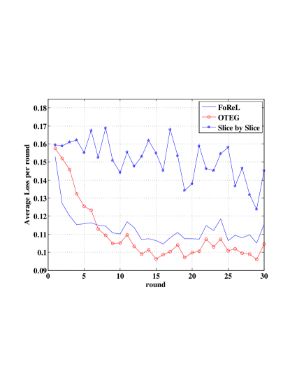
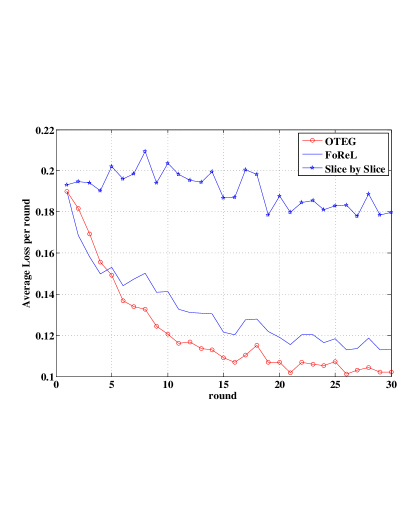
OTEG Experiment - Based on the collaborative filtering example in [3], we choose $\beta(k)=\sqrt{n+m}$ and $\tau(k)\approx 2||{\bm{\mathbf{{\widehat{M}}}}}^{(k)}||_{*}$. A small uniform random noise in $[0,5]$ is added to $\tau(k)$ to simulate imperfect a-priori knowledge of the tensor nuclear norm of $\bm{\mathscr{{M}}}$. Since a full implementation of OTEG requires solving a semi-definite program at each time step–which is computationally expensive and tedious to program–we opt to simplify the projection step of the algorithm. Specifically, instead of projecting onto $\widehat{\mathrsfs{W}}$, we project onto $\{\widehat{\bm{\mathscr{{W}}}}|\mathrm{Tr}(\mbox{\tt blkdiag}{(\widehat{\bm{\mathscr{{W}}}})})\leq\tau\}$ via trace normalization (a la Algo. 1 in [2]). This results in slower convergence, so to compensate the learning rate dictated by Algorithm 2 is increased by a factor of 8, i.e. $\eta=4\sqrt{\frac{\log(2(m+n))\sum_{k=1}^{d}\tau(k)}{TdG^{2}\sqrt{n+m}}}$. The lack of full projections also implies that $p_{t}$ is not necessarily in $[-1,1]$, so we cannot analytically calculate a Lipschitz constant for $l_{t}$. Instead, $G$ is the current maximum value of $|l_{t}^{\prime}(p_{t})|=|2(y_{t}-p_{t})|$ and is continuously updated (along with $\eta$) as the experiment progresses.

FoReL Experiment–FoReL is a standard approach to online convex optimization [5]. On each round $t$, we perform the update

$$\vspace{-1mm}\bm{\mathscr{{W}}}_{t+1}=\arg\min_{\bm{\mathscr{{W}}}}||\mathrsfs{P}_{t}(\bm{\mathscr{{W}}}-\bm{\mathscr{{M}}})||_{F}^{2}+\eta\sum_{k=1}^{d}||\widehat{{\bm{\mathbf{{W}}}}}^{(k)}||_{*}$$

Where $\mathrsfs{P}_{t}$ is a sampling operator that zeros out entries of a tensor corresponding to indices not yet sampled. This algorithm is implemented using FISTA [29] using 5 gradient descent iterations per update. We use the learning rate $\eta=\frac{B}{G\sqrt{T}}$, where $B=1.1||\bm{\mathscr{{M}}}||_{F}$ is an upper bound on $||\bm{\mathscr{{M}}}||_{F}$. $G$ is calculated in the same fashion as the OTEG experiment.

Completion slice by slice - We further compared our algorithm against the naive approach of slice by slice tensor completion where each slice was completed independently of each other (in the original domain).

The results of the three experiments are shown in Figure 3 for Dataset A and Dataset B respectively. The loss plots show a moving average of the value of $l_{t}(p_{t})$, where the $T$ time intervals are divided into $R=30$ rounds and we plot the average loss over each round. Note that while FoReL is better than OTEG in the first few rounds, OTEG seems to be slightly better than FoReL in the subsequent rounds. The reason for this is due to the fact that while solving for FoReL in each step we restrict the number of iterations to only 5 (for sake of reducing computation time). In other words we only partially solve the FoReL at each step. Also note that the slice by slice completion strategy is sub-optimal.

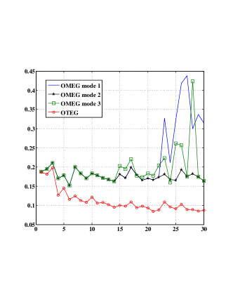
OMEG Experiment- A popular technique for tensor prediction is based on first flattening the tensor into a matrix followed by exploiting strategies for matrix completion. We will show here that such strategies are not necessarily optimal. We implement a version of the OMEG algorithm, [3], using OTEG but with the third dimension set to 1. The data for comparison is a reduced size data generated in the same manner as Dataset B with dimensions $50\times 60\times 20$. For OMEG, the 3-D data cube was flattened to a 2-D matrix in the 3 possible ways or modes, [18]. The total number of plays for this set-up was chosen to be $T=12,000$ which is about $20$% of the data. Note that the error performance of the best possible mode flattening for OMEG is well below the OTEG performance.

Figure 4: Loss plots for OTEG vs OMEG on a reduced size data cube. Note the superior performance of OTEG compared to OMEG

Discussion– Note the “total memory” approach of FoReL: every past sample is stored and used in calculating future updates. In contrast in OTEG implementation past plays are not stored and updates are calculated from only gradient information. While our implementation of OTEG stores all prior gradients, the full implementation theoretically requires only the latest gradient, which can be encoded with $g$ and $(i_{t},j_{t},k_{t})$. Taking into account the storage of $\bm{\mathscr{{W}}}_{t}$, this implies worst case OTEG memory consumption is $O((m+n)^{2}d)$, in contrast to $O(mnd+T)$ + Cost of storing past loss functions $l_{t}(\cdot)$ for FoReL. Note that in the current implementation of FoReL using FISTA one needs to recall all the past gradients (first order information only) of $\ell_{t}(\cdot)$ at each step. However, since the the loss function is fixed for all time steps for the current set of experiments, the memory cost of FoReL for our experiments is $O(mnd+T)$.

V-C Simulation Results on video data

Figure 5: Left to right: frame 1, 15, and 25. From top row to bottom row: Original video, FoReL, OTEG, OTEG with entries truncated to $[-1,1]$. Note the visual difference in performance.

We now experimentally demonstrate the effectiveness of OTEG on a 3-D video data. The test data, which we call $\bm{\mathscr{{M}}}$, is a 96x128x38 black and white video of a time-lapse city scene (Fig. 5), where each pixel is a light intensity in $[-1,1]$. The reason to choose this as the working example is because it can model dynamically changing rating matrices, and we can evaluate the performance visually. In particular, the shadow that propagates across the city can be seen as a “trend” emerging and fading in a time-dynamic collaborative filtering setting.

We simulate online learning of this data as follows: at time $t$, a pixel from the image is sampled at random from a uniform distribution among the set of pixels which have not yet been played, and this pixel is played as $y_{t}$. We apply two algorithms in this setup: (1) a partial implementation of OTEG, and (2) a standard follow-the-regularized-leader approach with tensor-nuclear-norm regularization.

Figure 6: Loss plots for OTEG and FoREL after 70000 iterations.

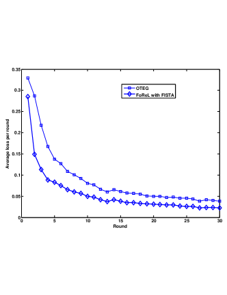
For both experiments, $n=96$, $m=128$, $d=38$ , $T=70000$ (15% of the video), and $l_{t}(p_{t})=(y_{t}-p_{t})^{2}$. The loss plots show a moving average of the value of $l_{t}(p_{t})$, where the $T$ time intervals are divided into $R=30$ rounds and we plot the average loss over each round.

Discussion–The loss plot and pictorial representation of frames 1,15, and 25 of the final iterate for both experiments are shown in Fig. 5 and Fig. 6. We see that in this case the FoReL algorithm achieves faster convergence, slightly better asymptotic performance, and better visual recovery of the image.

Figure 7: Loss plots for OTEG OMEG on a reduced size data cube. Note the superior performance of OTEG compared to OMEG.

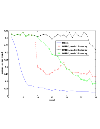
Comparison with Online Matrix Exponentiated Gradient (OMEG) Descent - We again implemented a version of the OMEG algorithm, [3], using OTEG but with the third dimension set to 1. The data for comparison was the same video as in the previous section but reduced to size $58\times 77\times 20$. For OMEG, the 3-D data cube was flattened to a 2-D matrix in the 3 possible ways or modes, [18]. The total number of plays for this set-up was chosen to be $T=17,864$ which is about $20$% of the data. Note that the error performance of the best possible mode flattening for OMEG is much worse than the OTEG performance.

VI Conclusion and Future Work

In this paper we presented an extension of strategies for online learning and prediction of matrices to tensors. Theoretical performance guarantees are derived which parallel the guarantees for the matrix case.

We demonstrated the utility of the proposed algorithm on several test cases. In future we will extend this work to consider higher order tensors and compare the performance with methods, which use different algebraic approaches for tensor factorization.

VII Appendix

Lemma VII.1.

For a real valued function $f$ with real valued domain defined via $f(\bm{\mathscr{{W}}})=\hat{f}(\widehat{\bm{\mathscr{{W}}}})$, the gradient $\nabla_{\bm{\mathscr{{W}}}}f(\bm{\mathscr{{W}}})=\mbox{\tt ifft}(\nabla_{\widehat{\bm{\mathscr{{W}}}}}\hat{f}(\widehat{\bm{\mathscr{{W}}}}),[\,],3).$

The proof of the Lemma follows from Lemma VII.2, which is a standard result in complex analysis.

Lemma VII.2.

Let $g:\mathbb{C}^{n}\to\mathbb{C}^{n}$ be holomorphic and $f:\mathbb{C}^{n}\to\mathbb{R}$ be real-differentiable. Then, the complex gradient of $f\circ g$ is given by

$$\nabla(f\circ g)=2\frac{\partial f(g)}{\partial\bar{z}}=(\nabla f){(\frac{\partial\bar{g}}{\partial\bar{z}})}$$

Proof is a simple consequence of the Cauchy-Riemann condition on $g$ and Equation (33) in [25]. We now prove Lemma VII.1.

Proof.

It will be helpful to re-parameterize $f$ as a function of an arbitrary tube ${\bm{\mathbf{w}}}_{ij}=\bm{\mathscr{{W}}}(i,j,:)$ and the remainder of the tensor $\bm{\mathscr{{W}}}_{\backslash{\bm{\mathbf{w}}}_{ij}}$. We let ${\bm{\mathbf{w}}}_{ij}$ be complex, and calculate the partial complex gradient $\nabla_{{\bm{\mathbf{w}}}_{ij}}f(\bm{\mathscr{{W}}})$. By Lemma VII.2, we have

$$\nabla_{{\bm{\mathbf{w}}}_{ij}}f(\bm{\mathscr{{W}}}) =\nabla_{\bm{\mathbf{w}}_{ij}}f(\bm{\mathscr{{W}}}_{\backslash{\bm{\mathbf{w}}}_{ij}},\bm{\mathbf{w}}_{ij})$$

$$=\nabla_{\bm{\mathbf{w}}_{ij}}\hat{f}(\widehat{\bm{\mathscr{{W}}}}_{\backslash{\hat{\bm{\mathbf{w}}}}_{ij}},{\bm{\mathbf{{F}}}}{{\bm{\mathbf{w}}}}_{ij})$$

$$=\nabla_{\bm{\mathbf{z}}}\hat{f}(\widehat{\bm{\mathscr{{W}}}}_{\backslash{\hat{\bm{\mathbf{w}}}}_{ij}},\bm{\mathbf{z}})(\frac{\partial}{\partial\bar{\bm{\mathbf{z}}}}\overline{{\bm{\mathbf{{F}}}}\bm{\mathbf{z}}})$$

$$=[\nabla_{\widehat{\bm{\mathscr{{W}}}}}\hat{f}(\widehat{\bm{\mathscr{{W}}}})](i,j,:)\overline{{\bm{\mathbf{{F}}}}}$$

Where the last equation follows from the fact that $\overline{{\bm{\mathbf{{F}}}}\bm{\mathbf{z}}}=\bar{{\bm{\mathbf{{F}}}}}\bar{\bm{\mathbf{z}}}$. To see that this proves the result, recall that we chose to represent a tube as a column vector, but this orientation was arbitrary. It follows that the row-vector interpretation of a tube will give

$$\nabla_{{\bm{\mathbf{w}}}_{ij}}f(\bm{\mathscr{{W}}}) =([\nabla_{\widehat{\bm{\mathscr{{W}}}}}\hat{f}(\widehat{\bm{\mathscr{{W}}}})](i,j,:)\bar{{\bm{\mathbf{{F}}}}})^{\top}$$

$$={\bm{\mathbf{{F}}}}^{\dagger}([\nabla_{\widehat{\bm{\mathscr{{W}}}}}\hat{f}(\widehat{\bm{\mathscr{{W}}}})](i,j,:))^{\top}$$

$$=\mbox{\tt ifft}([\nabla_{\widehat{\bm{\mathscr{{W}}}}}\hat{f}(\widehat{\bm{\mathscr{{W}}}})](i,j,:))$$

∎

VII-A The Block-Diagonal Linear $(\bm{\mathbf{\beta}},\bm{\mathbf{\tau}})$ Game

We consider a linear, positive-definite variation of Online Tensor Prediction, which has the same setup as in the previous Section. Let $\mathrsfs{S}\in\{\mathrsfs{A}\subseteq\mathrsfs{S}^{N\times N\times d}_{++}:\forall\bm{\mathscr{{W}}}\in\mathrsfs{A},\forall k:\mathrm{Tr}(\widehat{{\bm{\mathbf{{W}}}}}^{(k)})\leq\tau(k),\forall k\forall i:\widehat{{\bm{\mathbf{{W}}}}}^{(k)}(i,i)\leq\beta(k)\}$ be a set of positive-definite tensors with Fourier domain trace and diagonal-entry bounds $\bm{\mathbf{\tau}}$ and $\bm{\mathbf{\beta}}$, respectively. The loss functions $l_{t}$ will have the form $l_{t}(\bm{\mathscr{{W}}}_{t})=\mathrm{Tr}(\bm{\mathscr{{W}}}\star\bm{\mathscr{{L}}}_{t})=\mathrm{Tr}(\mbox{\tt blkdiag}(\widehat{\bm{\mathscr{{W}}}})\mbox{\tt blkdiag}(\widehat{\bm{\mathscr{{L}}}}_{t}))$ for tensors $\bm{\mathscr{{L}}}_{t}$. This problem is nearly identical to the linear game discussed in [3], except now every matrix is block-diagonal, and there is an independent $\beta$ and $\tau$ constraint for each block. Thus, we can apply the general regret bound derived for the original game, with slight modification. As required by the proof, we assume that the spectral norm $||\eta\mbox{\tt blkdiag}(\widehat{\bm{\mathscr{{L}}}}_{t})||\leq 1$ for all $t$.

Theorem VII.1.

Suppose Tensor Exponentiated Gradient is run on Linear Online Tensor Prediction. Then,

$$\mathrm{Regret}\leq\sum_{k=1}^{d}\{\eta\sum_{t=1}^{T}\mathrm{Tr}(\widehat{{\bm{\mathbf{{W}}}}}_{t}^{(k)}(\widehat{{\bm{\mathbf{{L}}}}}_{t}^{(k)})^{2})+\frac{\tau(k)\log{N}}{\eta}\}$$

The proof follows along the same lines as that of Theorem 10 in [3], except for the fact that we split trace operations by summing over the traces of each face. The fact that our matrices are complex does not matter, as the given proof is valid for all Hermitian matrices. Specifically, both the Golden Thompson inequality and the relation $\exp({\bm{\mathbf{{A}}}})\preceq{\bm{\mathbf{{I}}}}+{\bm{\mathbf{{A}}}}+{\bm{\mathbf{{A}}}}^{2}$ hold for general Hermitian ${\bm{\mathbf{{A}}}}$ with spectral norm $||{\bm{\mathbf{{A}}}}||\leq 1$. Note that for this result to be meaningful, we need to bound $\mathrm{Tr}((\widehat{{\bm{\mathbf{{L}}}}}_{t}^{(k)})^{2})$. Let us further assume, then, that $\mathrm{Tr}((\widehat{{\bm{\mathbf{{L}}}}}_{t}^{(k)})^{2})\leq\gamma(k)$ for some $\bm{\mathbf{\gamma}}\in\mathbb{R}^{d}$. For this scenario, Theorem VII.1 gives the following corollary.

Corollary VII.1.

Suppose TEG is run on $\bm{\mathbf{\gamma}}$-constrained Linear Online Tensor Prediction. Then,

$$\mathrm{Regret} \leq\sum_{k=1}^{d}\{\eta T\beta(k)\gamma(k)+\frac{\tau(k)\log{N}}{\eta}\}$$

$$=\eta T\sum_{k=1}^{d}\beta(k)\gamma(k)+\frac{\log N}{\eta}\sum_{k=1}^{d}\tau(k)$$

With this result in hand, we have a guide to deriving a bound for the general game, where loss functions are not necessarily linear.

VII-B Proof of Theorem IV.1

We first analyze Algorithm 2. For this we find a linear approximation of the regret, which will permit us to use Corollary VII.1. For any $\bm{\mathscr{{U}}}\in\mathrsfs{S}$, note that

$$\mathrm{Tr}(\mbox{\tt blkdiag}(\widehat{\phi}(\bm{\mathscr{{U}}}))\mbox{\tt blkdiag}(\widehat{\bm{\mathscr{{L}}}}_{t}))$$

$$=g\sum_{k=1}^{d}(\widehat{{\bm{\mathbf{{P}}}}}^{(k_{t})}(i_{t},j_{t})-\widehat{{\bm{\mathbf{{N}}}}}^{(k_{t})}(i_{t},j_{t}))\overline{{\bm{\mathbf{{F}}}}}(k,k_{t})$$

$$\hskip 28.45274pt+(\widehat{{\bm{\mathbf{{P}}}}}^{(k_{t})}(j_{t},i_{t})-\widehat{{\bm{\mathbf{{N}}}}}^{(k_{t})}(j_{t},i_{t})){\bm{\mathbf{{F}}}}(k,k_{t})$$

$$=\frac{g}{\sqrt{d}}\sum_{k=1}^{d}\widehat{{\bm{\mathbf{{U}}}}}^{(k_{t})}(i_{t},j_{t})e^{\frac{2\pi i(k-1)(k_{t}-1)}{d}}$$

$$\hskip 34.1433pt+\widehat{{\bm{\mathbf{{U}}}}}^{(k_{t})\dagger}(i_{t},j_{t})e^{\frac{-2\pi i(k-1)(k_{t}-1)}{d}}$$

$$=2g\ \mbox{\tt ifft}(\widehat{\bm{\mathscr{{U}}}})(i_{t},j_{t},k_{t})=2g\bm{\mathscr{{U}}}(i_{t},j_{t},k_{t})$$

We see that the linear loss $\mathrm{Tr}(\mbox{\tt blkdiag}(\widehat{\bm{\mathscr{{W}}}})\mbox{\tt blkdiag}(\widehat{\bm{\mathscr{{L}}}}_{t}))$ is equivalent to $2gP_{\widehat{\bm{\mathscr{{W}}}}}(i_{t},j_{t},k_{t})$, and thus

$$\mathrm{Tr}(\mbox{\tt blkdiag}(\widehat{\bm{\mathscr{{W}}}})\mbox{\tt blkdiag}(\widehat{\bm{\mathscr{{L}}}}_{t})) =2gP_{\widehat{\bm{\mathscr{{W}}}}_{t}}(i_{t},j_{t},k_{t})=2gp_{t}$$

This implies that,

$$\mathrm{Tr}(\mbox{\tt blkdiag}(\widehat{\bm{\mathscr{{W}}}})\mbox{\tt blkdiag}(\widehat{\bm{\mathscr{{L}}}}_{t}))-\mathrm{Tr}(\mbox{\tt blkdiag}(\widehat{\phi}(\bm{\mathscr{{U}}}))\mbox{\tt blkdiag}(\widehat{\bm{\mathscr{{L}}}}_{t}))$$

$$=2g(p_{t}-\bm{\mathscr{{U}}}(i_{t},j_{t},k_{t}))\geq 2(l_{t}(p_{t})-l_{t}(\bm{\mathscr{{U}}}(i_{t},j_{t},k_{t})))$$

By convexity of $l_{t}$. Thus, the regret of our algorithm is at most half the regret of the linear game with loss tensors $\widehat{\bm{\mathscr{{L}}}}_{t}$.

Assuming $\eta||\mbox{\tt blkdiag}(\widehat{\bm{\mathscr{{L}}}}_{t})||\leq 1$, we apply Corollary VII.1 to obtain

$$\mathrm{Regret} \leq\frac{1}{2}\mathrm{Regret}_{\mathrm{Linear}}$$

$$\leq\frac{1}{2}\left\{4G^{2}\eta T\sum_{k=1}^{d}\beta(k)+\frac{\log N}{\eta}\sum_{k=1}^{d}\tau(k)\right\}$$

Setting $\eta=\sqrt{\frac{\log N\sum_{k=1}^{d}\tau(k)}{4G^{2}T\sum_{k=1}^{d}\beta(k)}}$, we have

$$\mathrm{Regret} \leq\frac{1}{2}\left\{2\sqrt{4G^{2}T\log N(\sum_{k=1}^{d}\beta(k))(\sum_{k=1}^{d}\tau(k))}\right\}$$

$$=2G\sqrt{T\log N(\sum_{k=1}^{d}\beta(k))(\sum_{k=1}^{d}\tau(k))}$$

Which gives us the stated bound.

We now address the technical condition that $\eta||\mbox{\tt blkdiag}(\widehat{\bm{\mathscr{{L}}}}_{t})||\leq 1$. Let $k_{0}=\arg\max_{k\in[d]}||\widehat{{\bm{\mathbf{{L}}}}}^{(k)}_{t}||$. We have $||\mbox{\tt blkdiag}(\widehat{\bm{\mathscr{{L}}}}_{t})||=\max_{k\in[d]}||\widehat{{\bm{\mathbf{{L}}}}}^{(k)}_{t}||=||\widehat{{\bm{\mathbf{{L}}}}}_{t}^{(k_{0})}||\leq||\widehat{{\bm{\mathbf{{L}}}}}_{t}^{(k_{0})}||_{F}=\sqrt{\mathrm{Tr}((\widehat{{\bm{\mathbf{{L}}}}}_{t}^{(k_{0})})^{2})}\leq\sqrt{\gamma(k_{0})}=\sqrt{4G^{2}}$. For $T\geq\frac{\log N\sum_{k=1}^{d}\tau(k)}{\sum_{k=1}^{d}\beta(k)}$ and our choice of $\eta$, this implies $\eta||\mbox{\tt blkdiag}(\widehat{{\bm{\mathbf{{L}}}}}_{t})||\leq 1$, and the bound holds.

For $T<\frac{\log N\sum_{k=1}^{d}\tau(k)}{\sum_{k=1}^{d}\beta(k)}$, note that $l_{t}$ have derivatives bounded by $G$, and the domain is $[-1,1]$, so the maximum possible regret on any round is $2G$. Hence the regret up to time $T$ is at most $2GT<2G\sqrt{T\log N(\sum_{k=1}^{d}\beta(k))(\sum_{k=1}^{d}\tau(k))}$, since $||\beta||_{1}\geq 1$.

References

- [1] Misha E. Kilmer and Carla D. Martin, “Factorization strategies for third-order tensors,” Linear Algebra and its Applications, vol. Special Issue in Honor of G. W. Stewart’s 70th birthday, Vol. 435, no. 3, pp. 641–658, 2011.
- [2] Koji Tsuda, Gunnar Ratsch, and Manfred K Warmuth, “Matrix exponentiated gradient updates for on-line learning and bregman projection,” The Journal of Machine Learning Research, vol. 6, Dec. 2005.
- [3] Elad Hazan, Satyen Kale, and Shai Shalev-Shwartz, “Near-optimal algorithms for online matrix prediction,” in COLT, 2012, pp. 38.1–38.13.
- [4] Nicolo Cesa-Bianchi and Gabor Lugosi, Prediction, Learning, and Games, Cambridge University Press, 2006.
- [5] Shai Shalev-Shwartz, “Online Learning and Online Convex Optimization,” Foundations and Trends® in Machine Learning, vol. 4, no. 2, pp. 107–194, 2012.
- [6] Yehuda Koren, “Collaborative filtering with temporal dynamics,” Commun. ACM, vol. 53, no. 4, pp. 89–97, 2010.
- [7] Ohad Shamir and Shai Shalev-Shwartz, “Collaborative filtering with the trace norm: Learning, bounding, and transducing,” in COLT, 2011, pp. 661–678.
- [8] Sham M. Kakade, Shai Shalev-Shwartz, and Ambuj Tewari, “Regularization techniques for learning with matrices,” Journal of Machine Learning Research, vol. 13, pp. 1865–1890, 2012.
- [9] Benjamin Recht, Maryam Fazel, and Pablo A. Parrilo, “Guaranteed minimum-rank solutions of linear matrix equations via nuclear norm minimization,” SIAM Rev., vol. 52, no. 3, pp. 471–501, Aug. 2010.
- [10] M. Kilmer, K. Braman, N. Hao, and R. Hoover, “Third-order tensors as operators on matrices: A theoretical and computational framework with applications in imaging,” SIAM Journal on Matrix Analysis and Applications, vol. 34, no. 1, pp. 148–172, 2013.
- [11] Zemin Zhang, Gregory Ely, Shuchin Aeron, Ning Hao, and Misha Kilmer, “Novel methods for multilinear data completion and de-noising based on tensor-svd,” in Computer Vision and Pattern Recognition (CVPR), 2014 IEEE Conference on. IEEE, 2014, pp. 3842–3849.
- [12] Gregory Ely, Shuchin Aeron, Ning Hao, and Misha E Kilmer, “5D and 4D pre-stack seismic data completion using tensor nuclear norm (TNN),” in Society of Exploration Geophysicists (SEG) workshop, 2013.
- [13] Tamara G. Kolda and Brett W. Bader, “Tensor decompositions and applications,” SIAM REVIEW, vol. 51, no. 3, pp. 455–500, 2009.
- [14] Wolfgang Hackbusch, Tensor Spaces and Numerical Tensor Calculus, Springer Series in Computational Mathematics, Vol. 42. Springer, 2012.
- [15] T.G. Kolda and B.W. Bader, “Tensor decompositions and applications,” SIAM Review, vol. 51, no. 3, pp. 455–500, 2009.
- [16] P. Jain and S. Oh, “Provable Tensor Factorization with Missing Data,” ArXiv e-prints, June 2014.
- [17] Daniel Kressner, Michael Steinlechner, and Bart Vandereycken, “Low-rank tensor completion by riemannian optimization,” BIT Numerical Mathematics, vol. 54, no. 2, pp. 447–468, 2014.
- [18] Ryota Tomioka, Taiji Suzuki, Kohei Hayashi, and Hisashi Kashima, “Statistical performance of convex tensor decomposition,” in NIPS, 2011, pp. 972–980.
- [19] A. Krishnamurthy and A. Singh, “Low-Rank Matrix and Tensor Completion via Adaptive Sampling,” ArXiv e-prints, Apr. 2013.
- [20] C. Navasca, M. Opperman, T. Penderghest, and C. Tamon, “Tensors as module homomorphisms over group rings,” ArXiv e-prints, May 2010.
- [21] N. Hao, M. Kilmer, K. Braman, and R. Hoover, “Facial recognition using tensor-tensor decompositions,” SIAM Journal on Imaging Sciences, vol. 6, no. 1, pp. 437–463, 2013.
- [22] Karen Braman, “Third-order tensors as linear operators on a space of matrices,” Linear Algebra and its Applications, pp. 1241–1253, 2010.
- [23] I. Dhillon and J. Tropp, “Matrix nearness problems with bregman divergences,” SIAM Journal on Matrix Analysis and Applications, vol. 29, no. 4, pp. 1120–1146, 2008.
- [24] A S Lewis, “Convex analysis on the Hermitian matrices,” SIAM Journal on Optimization, vol. 6, no. 1, pp. 164–177, 1996.
- [25] K. Kreutz-Delgado, “The Complex Gradient Operator and the CR-Calculus,” ArXiv e-prints, June 2009.
- [26] “Movie lens database,” http://grouplens.org/datasets/movielens/.
- [27] Jure Leskovec and Rok Sosič, “SNAP: A general purpose network analysis and graph mining library in C++,” http://snap.stanford.edu/snap, June 2014.
- [28] Ali Jadbabaie, Pooya Molavi, and Alireza Tahbaz-Salehi, “Information heterogeneity and the speed of learning in social networks,” Tech. Rep. No. 13-28, Columbia Business School Research Paper, 2013, SSRN: http://ssrn.com/abstract=2266979 or http://dx.doi.org/10.2139/ssrn.2266979.
- [29] Amir Beck and Marc Teboulle, “A Fast Iterative Shrinkage-Thresholding Algorithm for Linear Inverse Problems,” SIAM Journal on Imaging Sciences, vol. 2, no. 1, pp. 183–202, Jan 2009.