Composite Learning Control With Application
to Inverted Pendulums
Abstract
Composite adaptive control (CAC) that integrates direct and indirect adaptive control techniques can achieve smaller tracking errors and faster parameter convergence compared with direct and indirect adaptive control techniques. However, the condition of persistent excitation (PE) still has to be satisfied to guarantee parameter convergence in CAC. This paper proposes a novel model reference composite learning control (MRCLC) strategy for a class of affine nonlinear systems with parametric uncertainties to guarantee parameter convergence without the PE condition. In the composite learning, an integral during a moving-time window is utilized to construct a prediction error, a linear filter is applied to alleviate the derivation of plant states, and both the tracking error and the prediction error are applied to update parametric estimates. It is proven that the closed-loop system achieves global exponential-like stability under interval excitation rather than PE of regression functions. The effectiveness of the proposed MRCLC has been verified by the application to an inverted pendulum control problem.
I Introduction
Adaptive control is one of the major control techniques of handling uncertainties in nonlinear systems and has still attracted great concern in recent years [1, 2, 3, 4, 5, 6, 7, 8, 9, 10, 11, 12, 13, 14, 15, 16]. In particular, model reference adaptive control (MRAC) is a popular adaptive control architecture which aims to make an uncertain dynamical system behave like a chosen reference model. The way of parameter estimation in adaptive control gives rise to two different schemes, namely indirect and direct schemes [17]. Composite adaptive control (CAC) is an integrated direct and indirect adaptive control technique which aims to achieve better tracking and parameter estimation through faster and smoother parameter adaptation [18]. In the CAC, prediction errors are generated by identification models, and both tracking errors and prediction errors are applied to update parametric estimates. The superiority of CAC on performance improvement has been demonstrated in many control designs, where some latest results can be referred to [19, 21, 22, 20, 23, 24, 25, 26]. Nevertheless, as in the classical adaptive control, CAC only achieves asymptotic convergence of tracking errors and does not guarantee parameter convergence unless plant states satisfy the condition of persistent excitation (PE) [17]. It is well known that the PE condition is very strict and often infeasible to monitor online in practical control systems [27].
Learning is one of the fundamental features of autonomous intelligent behavior, and it is closely related to parameter convergence in adaptive control [30]. The benefits brought by parameter convergence include accurate closed-loop identification, exponential stability and robustness against measurement noise [28]. An emerging concurrent learning technique provides a feasible and promising way for achieving parameter convergence without the PE condition in MRAC [27, 29, 28]. The difference between the concurrent learning and the composite adaptation lies in how to construct prediction errors. In the concurrent learning, a dynamic data stack constituted by online recorded data is used in constructing prediction errors, singular value maximization is applied to maximize the singular value of the data stack, and exponential convergence of both tracking errors and estimation errors is guaranteed if regression functions of plant uncertainties are excited over a time interval such that sufficiently rich data are recorded in the data stack. Yet in this innovative design, the singular value maximization leads to an exhaustive search over all recorded data, and the requirement on the derivation of all plant states for calculating prediction errors is stringent.
This paper proposes a novel model reference composite learning control (MRCLC) strategy for a class of parametric uncertain affine nonlinear systems. In the composite learning, a modified modelling error that can utilize online recorded data is constructed as the prediction error, a second-order command filter is applied to alleviate the derivation of plant states, and both the tracking error and the prediction error are applied to update parametric estimates. It is proven that the closed-loop system achieves global exponential-like stability under interval excitation (IE) rather than PE of regression functions. Consequently, the limitations of concurrent learning are alleviated by the proposed MRCLC design. The effectiveness and superiority of this approach is verified by the application to an inverted pendulum control problem with the comparison with some existing adaptive control approaches.
The notations of this paper are relatively standard, where , , and denote the spaces of real numbers, positive real numbers, real -dimensional vectors, and -dimensional matrixes, respectively, and denote the absolute value and Euclidean-norm, respectively, denotes the space of bounded signals, denotes the ball of radius , and are the minimum and maximum functions, respectively, sgn is the sign function, rank is the rank of , diag is a diagonal matrix, and represents the space of functions whose -order derivatives all exist and are continuous, where , , , and , and are positive integers.
II Problem Formulation
This section discusses the formulation of learning from the classical MRAC. For clear illustration, consider a class of nth order affine nonlinear systems as follows [27]:
| (1) |
where , , , is the vector of plant states, is the control input, and is the model uncertainty. A reference model that characterizes the desired response of the system (1) is given by
| (2) |
with , in which is a strictly Hurwitz matrix, is the vector of reference model states, and is a bounded reference signal. This study is based on the facts that is measurable, is controllable, and is linearly parameterizable such that [27, 29, 28]
| (3) |
in which is a unknown constant parameter vector, is a known regression function vector, and is a known constant. The following definitions are given for facilitating control synthesis.
Definition 1 [27]: A bounded signal is of IE over if there exist constants with such that holds.
Definition 2 [27]: A bounded signal satisfies the PE condition if there exist constants such that holds, .
Let be an augmented reference signal, and be an estimate of . Define a tracking error , and an estimation error . Our objective is to design a proper parametric update law of MRAC such that both and exponentially converge to 0 under the IE rather than the PE conation.
III Composite Learning Control Strategy
III-A Review of Previous Results
From [17], the MRAC law can be designed as follows:
| (4) | ||||
where denotes a proportional-derivative (PD) feedback part, denotes a reference signal feedforward part, denotes an adaptive part, and are control gains, and the design of satisfies
| (5) |
Thus, one obtains the tracking error dynamics
| (6) |
where is designed to be strictly Hurwitz. Thus, for any matrix , a unique solution exists for the following Lyapunov equation:
| (7) |
Let the adaptive law of be as follows:
| (8) |
where is a learning rate, and is a projection operator given by [17]
Choose a Lyapunov function candidate
| (9) |
with for the closed-loop dynamics composed of (6) and (8). It follows from the classical MRAC result of [17] that if and is of PE, then the closed-loop system (6) with (8) achieves global exponential stability in the sense that both the tracking error and the estimation error converge to 0.
To remove the requirement of the PE condition on for parameter convergence in [17], a concurrent learning law of is proposed in [27] as follows:
| (10) |
where is a certain epoch, is the number of stored data, and denotes a modelling error which is regarded as the prediction error calculated by
| (11) |
where , and are online recorded data of , and at the epoch , respectively. Let be a dynamic data stack. It is shown in the concurrent learning MRAC approach of [27] that if and rank on , then the closed-loop system (6) with (10) achieves global exponential-like stability in the sense that both the tracking error and the estimation error converge to 0 on . Yet in the approach of [27], fixed-point smoothing must be applied to estimate in (11) such that the prediction error is calculable, and singular value maximization should be applied to exhaustively search the data stack to maximize its singular value.
III-B Composite Learning Control Design
Define a modified modelling error as the prediction error, in which
| (12) |
with and
| (13) |
in which is an integral duration, is the minimal singular value of , and is the time when reaches its maximum111The presence of and here is only used in the subsequent performance analysis and their values can only be gotten at the control process.. Then, a composite learning law of is designed as follows:
| (14) |
in which is a weight factor.
From and (12), the calculation of can follow the calculation of as follows:
| (15) |
where is directly obtainable by (13) and (14), and is not directly obtainable. Multiplying both sides of (6) by , integrating the resulting equality over and making some transformations, one gets
| (16) |
in which the time variable is omitted in the above integral part. Since is unavailable, a second-order linear filter with unit gain is implemented as follows [31]:
| (17) |
with and , where is the natural frequency, is the damping factor, and and are estimates of and , respectively. The integral in (16) effectively reduces the influence of measurement noise on the calculation of . Thus, in (17) can be made sufficiently small so that . For simplifying analysis, assume that as in [31]. The reasonability of this assumption will also be verified in the subsequent simulations. The following theorem shows the main result of this study.
Theorem 1: Consider the system (1) driven by the control law (4) with (14), where the control gain is designed to satisfy (5), and the control gain is selected to make in (6) strictly Hurwitz. If and are satisfied with and , then the closed-loop system composed of (6) and (14) achieves global exponential-like stability in the sense that all closed-loop signals are bounded for all and both the tracking error and the estimation error exponentially converge to 0 on .
proof: Firstly, consider the control problem at . Choose the Lyapunov function candidate in (9) for the closed-loop system constituted by (6) and (14). The time derivative of along (6) is as follows:
| (18) |
where (7) is utilized to obtain (18). Applying (14) to (18), noting and , and using the projection operator results in [17], one obtains
| (19) |
Noting and , one gets , , which implies that the closed-loop system is stable in the sense that . Since is satisfied and in (9) is radially unbounded (i.e. as ), the stability is global. Using , one also obtains from their definitions. Thus, all closed-loop signals are bounded for all .
Secondly, consider the control problem at . since there exist and such that , i.e. the bounded signal is exciting over , it is obtained from (19) that
| (20) |
It follows from (9) and (20) that
| (21) |
where , which implies that the closed-loop system has global exponential-like stability in the sense that both and exponentially converge to 0 as long as .
IV Application to Inverted Pendulum
Consider the following inverted pendulum model [27]:
in which and , . The reference model is given as follows:
For simulations, set , while , and while [27].
The parameters selection of the proposed control law (4) with (14) is based on that of [27], where the details are given as follows: firstly, solve (5) to obtain ; secondly, select so that is strictly Hurwitz; thirdly, solve (7) with to obtain ; fourthly, set 5 s in (13); fifthly, set 3.5, 6 and 5 in (14); finally, set 100 and 0.7 in (17).
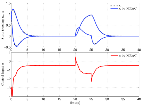
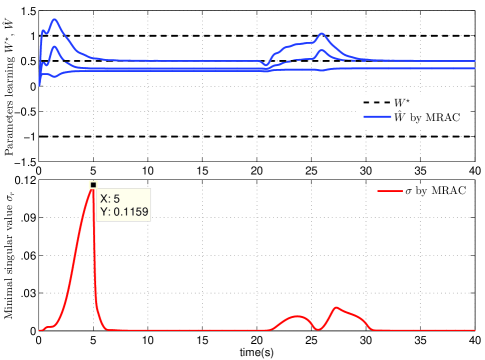
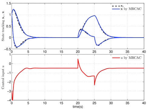
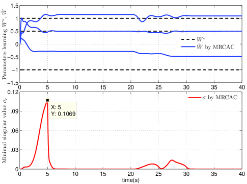
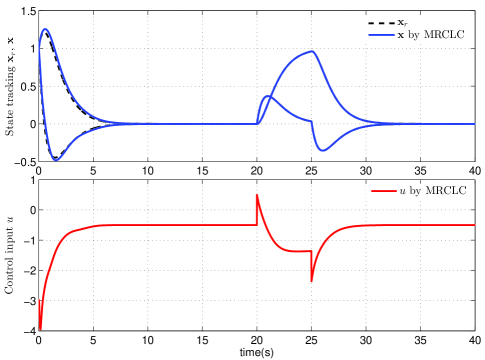
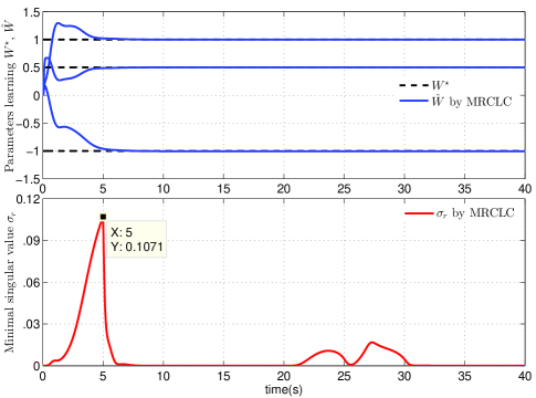
Simulations are carried out in MATLAB software running on Windows 7, where the solver is set to be fixed-step ode 5 with the step size being 0.001 s and other settings being default values. The conventional MRAC in [17] and the model reference CAC (MRCAC) with Q-modification in [32] are selected as baseline controllers, where the reference models and shared parameters of all controllers are set to be the same for fair comparisons. Simulation trajectories by all controllers are depicted Fig. 1. For the control performance, it is shown that the plant state follows its desired signal closely with a smooth control input for all controllers, the MRCAC achieves the worst tracking accuracy [see Fig. 1(c)], and the proposed MRCLC achieves the best tracking accuracy [see Fig. 1(e)]. For the learning performance, it is observed that IE occurs with rising at s in this case, the MRAC does not show any parameter convergence [see Fig. 1(b)], the MRCLC shows better parameter estimation than the MRAC but still does not achieve parameter convergence [see Fig. 1(d)], and the proposed MRCLC achieves fast and accurate parameter estimation even the IE is short and weak [see Fig. 1(f)].
V Conclusion
In this paper, a MRCLC strategy has been successfully developed for a class of parametric uncertain affine nonlinear systems such that parameter convergence can be guaranteed by the IE rather than PE condition. The proposed approach has also been applied to an inverted pendulum model, where superior control and learning performances have been demonstrated compared with the conventional MRAC and the MRCAC with Q-modification. Further work would focus on the extension of the composite learning to wider classes of nonlinear systems such as multi-input multi-output affine nonlinear systems [34] and strict-feedback nonlinear systems [35].
Acknowledgment
This work was supported in part by the National Research Foundation of Singapore under Grant NRF2014NRF-POC001-027, in part by the Biomedical Engineering Programme, Agency for Science, Technology and Research (A*STAR), Singapore under Grant 1421480015, and in part by AFR and FNR programs, Luxembourg.
References
- [1] K. J. Astrom and B. Wittenmark, Adaptive Control, 2nd ed. Mineola, NY, USA: Dover, 2008.
- [2] A. Astolfi, D. Karagiannis, and R. Ortega, Nonlinear and Adaptive Control with Applications. London, UK: Springer, 2008.
- [3] B. D. O. Anderson and A. Dehghani, “Challenges of adaptive control-past, permanent and future,” Annu. Rev. Control, vol. 32, no. 2, pp. 123-135, Dec. 2008.
- [4] M. Stefanovic and M. G. Safonov, Safe Adaptive Control: Data-Driven Stability Analysis and Robust Synthesis. London, UK: Springer, 2011.
- [5] K. S. Narendra and Z. Han, “The changing face of adaptive control: The use of multiple models,” Annu. Rev. Control, vol. 35, no. 1, pp. 1- 12, Apr. 2011.
- [6] A. Casavola, J. Hespanha, and P. Ioannou, “Special issue on ‘recent trends on the use of switching and mixing in adaptive control’,” Int. J. Adapt. Control Signal Process., vol. 26, no. 8, pp. 690-691, Aug. 2012.
- [7] S. G. Khan, G. Herrmann, F. L. Lewis, T. Pipe, and C. Melhuish, “Reinforcement learning and optimal adaptive control: An overview and implementation examples,” Annu. Rev. Control, vol. 36, no. 1, pp. 42-59, Apr. 2012.
- [8] J. M. Martin-Sanchez, J. M. Lemos, and J. Rodellar, “Survey of industrial optimized adaptive control,” Int. J. Adapt. Control Signal Process., vol. 26, no. 10, pp. 881-918, Oct. 2012.
- [9] K. B. Pathak and D. M. Adhyaru, “Survey of model reference adaptive control,” in Proc. Nirma University International Conference on Engineering, Ahmedabad, India, 2012, pp. 1-6.
- [10] E. Lavretsky and K. A. Wise, Robust and Adaptive Control: With Aerospace Applications. London, UK: Springer, 2013.
- [11] A. Serrani, “An output regulation perspective on the model reference adaptive control problem,” Int. J. Adapt. Control Signal Process., vol. 27, no. 1-2, pp. 22-34, Jan. 2013.
- [12] J. Sun, M. Krstic, and N. Bekiaris-Liberis, “Robust adaptive control: legacies and horizons,” Int. J. Adapt. Control Signal Process., vol. 27, no. 1-2, pp. 1-3, Jan. 2013.
- [13] I. Barkana, “Simple adaptive control - a stable direct model reference adaptive control methodology - brief survey,” Int. J. Adapt. Control Signal Process., vol. 28, no. 7-8, pp. 567-603, Jul. 2014.
- [14] L. P. Chan, F. Naghdy, and D. Stirling, “Application of adaptive controllers in teleoperation systems: A survey,” IEEE Trans. Hum.-Mach. Syst., vol. 44, no. 3, pp. 337-352, Jun. 2014.
- [15] P. Swarnkar, S. K. Jain, and R. K. Nema, “Adaptive control schemes for improving the control system dynamics: A review,” IETE Tech. Rev., vol. 31, no. 1, pp. 17-33, Jan-Feb. 2014.
- [16] G. Tao, “Multivariable adaptive control: A survey,” Automatica, vol. 50, no. 11, pp. 2737-2764, Nov. 2014.
- [17] P. A. Ioannou and J. Sun, Robust Adaptive Control. Englewood Cliffs, NJ: Prentice Hall, 1996.
- [18] J.-J. E. Slotine and W. Li, “Composite adaptive control of robot manipulators,” Automatica, vol. 25, no. 4, pp. 509-519, Jul. 1989.
- [19] D. Naso, F. Cupertino, and B. Turchiano, “Precise position control of tubular linear motors with neural networks and composite learning,” Control Eng. Practice, vol. 18, no. 5, pp. 515-522, May 2010.
- [20] A. Mohanty and B. Yao, “Integrated direct/indirect adaptive robust control of hydraulic manipulators with valve deadband,” IEEE-ASME Trans. Mechatron., vol. 16, no. 4, pp. 707-715, Aug. 2011.
- [21] P. M. Patre, S. Bhasin, Z. D. Wilcox, and W. E. Dixon, “Composite adaptation for neural network-based controllers,” IEEE Trans. Autom. Control, vol. 55, no. 4, pp. 944-950, Apr. 2010.
- [22] C. Hu, B. Yao, and Q. Wang, “Integrated direct/indirect adaptive robust contouring control of a biaxial gantry with accurate parameter estimations,” Automatica, vol. 46, no. 4, pp. 701-707, Apr. 2010.
- [23] Y. P. Pan, M. J. Er, and T. R. Sun, “Composite adaptive fuzzy control for synchronizing generalized Lorenz systems,” Chaos, vol. 22, no. 2, Article ID 023144, Jun. 2012.
- [24] Y. P. Pan, Y. Zhou, T. R. Sun, and M. J. Er, “Composite adaptive fuzzy tracking control of uncertain nonlinear systems,” Neurocomputing, vol. 99, pp. 15-24, Jan. 2013.
- [25] X. J. Wei, N. Chen, and W. Q. Li, “Composite adaptive disturbance observer-based control for a class of nonlinear systems with multisource disturbance,” Int. J. Adapt. Control Signal Process., vol. 27, no. 3, pp. 199-208, Mar. 2013.
- [26] Z. T. Dydek, A. M. Annaswamy, J. J. E. Slotine, and E. Lavretsky, “Composite adaptive posicast control for a class of LTI plants with known delay,” Automatica, vol. 49, pp. 1914-1924, Jun. 2013.
- [27] G. V. Chowdhary and E. N. Johnson, “Concurrent learning for convergence in adaptive control without persistency of excitation,” in Proc. IEEE Conf. Decision Control, Atlanta, GA, 2010, pp. 3674-3679.
- [28] G. V. Chowdhary, M. Muhlegg, and E. N. Johnson,“Exponential parameter and tracking error convergence guarantees for adaptive controllers without persistency of excitation,” Int. J. Control, vol. 87, no. 8, pp. 1583-1603, May 2014.
- [29] G. V. Chowdhary and E. N. Johnson, “Theory and flight-test validation of a concurrent-learning adaptive controller,” J. Guid. Control Dyn., vol. 34, no. 2, pp. 592-607, 2011.
- [30] P. J. Antsaklis, “Intelligent learning control,” IEEE Control Syst. Mag., vol. 15, no. 3, pp. 5-7, Jun. 1995.
- [31] J. C. Hu and H. H. Zhang, “Immersion and invariance based command-filtered adaptive backstepping control of VTOL vehicles,” Automatica, vol. 49, no. 7, pp. 2160-2167, Jul. 2013.
- [32] K. Y. Volyanskyy, W. M. Haddad, and A. J. Calise, “A new neuroadaptive control architecture for nonlinear uncertain dynamical systems: beyond - and e-modifications,” IEEE Trans. Neural Netw., vol. 20, no. 11, pp. 1707-1723, Nov. 2009.
- [33] S. V. Joshi, A. Sreenatha, and J. Chandrasekhar, “Suppression of wing rock of slender delta wings using a single neuron controller,” IEEE Trans. Autom. Control Syst. Tech., vol. 6, pp. 671-677, Sep. 1998.
- [34] Y. P. Pan and M. J. Er, “Enhanced adaptive fuzzy control with optimal approximation error convergence,” IEEE Trans. Fuzzy Syst., vol. 21, no. 6, pp. 1123-1132, Dec. 2013.
- [35] Y. P. Pan and H. Y. Yu, “Dynamic surface control via singular perturbation analysis,” Automatica,vol. 51, pp. 29-33, Jul. 2015.