Toward Accurate Modeling of the Nonlinear Matter Bispectrum: Standard Perturbation Theory and Transients from Initial Conditions

Abstract

Accurate modeling of nonlinearities in the galaxy bispectrum, the Fourier transform of the galaxy three-point correlation function, is essential to fully exploit it as a cosmological probe. In this paper, we present numerical and theoretical challenges in modeling the nonlinear bispectrum. First, we test the robustness of the matter bispectrum measured from $N$-body simulations using different initial conditions generators. We run a suite of $N$-body simulations using the Zel’dovich approximation and second-order Lagrangian perturbation theory (2LPT) at different starting redshifts, and find that transients from initial decaying modes systematically reduce the nonlinearities in the matter bispectrum. To achieve $1\%$ accuracy in the matter bispectrum at $z\leq 3$ on scales $k<1$ $h$/Mpc, 2LPT initial conditions generator with initial redshift $z\gtrsim 100$ is required. We then compare various analytical formulas and empirical fitting functions for modeling the nonlinear matter bispectrum, and discuss the regimes for which each is valid. We find that the next-to-leading order (one-loop) correction from standard perturbation theory matches with $N$-body results on quasi-linear scales for $z\geq 1$. We find that the fitting formula in Gil-Marín et al. (2012) accurately predicts the matter bispectrum for $z\leq 1$ on a wide range of scales, but at higher redshifts, the fitting formula given in Scoccimarro & Couchman (2001) gives the best agreement with measurements from $N$-body simulations.

1 Introduction

The large-scale structure of matter and galaxies in the Universe is an excellent cosmological probe. Thus far, the two-point correlation function of galaxies has been widely employed to study the large-scale structure, and broaden our understanding of the Universe by providing tight constraints on, e.g., the curvature of the Universe, initial conditions, and properties of dark energy (e.g. (Tegmark et al., 2006; Blake et al., 2011; Parkinson et al., 2012; Reid et al., 2012; de la Torre et al., 2013)). A complete description of non-Gaussian large-scale structure, however, must include higher-order statistics. Although the matter density fluctuations follow nearly Gaussian statistics at early times, the nonlinear process of gravitational instability generically drives the matter density non-Gaussian. In addition, a nonlinear relation (bias) between the galaxy density and matter-density contrast and the distortion of the measured redshift of galaxies due to peculiar velocity further enhance the non-Gaussianity. The leading order statistic sensitive to such non-Gaussianity is the three-point correlation function, or its Fourier transform the bispectrum.

The galaxy three-point function and bispectrum have been measured previously in IRAS (Scoccimarro et al., 2001), 2dFGRS (Verde et al., 2002; Gaztañaga et al., 2005), SDSS (Nichol et al., 2006; Nishimichi et al., 2007; Marín, 2011; McBride et al., 2011a, b; Gil-Marín et al., 2015), and WiggleZ (Marín et al., 2013), but have not been as fruitful as their two-point counterparts because theoretical modeling of higher-point statistics has not yet reached the level that is required for sophisticated data analysis. Future surveys promise orders of magnitude improvement in both galaxy number density and volume coverage, permitting better determination of the higher-order statistics of the cosmic density field, and the huge resources that the community has put into those large surveys compels us to exploit the higher order statistics. Upon accessing all the cosmological information, the three-point statistics will be a powerful probe of inflation (Jeong & Komatsu, 2009; Sefusatti & Komatsu, 2007; Baldauf et al., 2011), nonlinear structure formation (Scoccimarro et al., 1998, 1999), and astrophysics such as galaxy formation (Baldauf et al., 2011).

In order to extract information from the bispectrum of galaxies we must have an accurate model of the bispectrum of the underlying matter field. Cosmological $N$-body simulations are the most direct way of studying the nonlinear evolution of the matter bispectrum. One consideration when modeling the bispectrum using simulations (in particular at high redshift) is transients from initial conditions (Scoccimarro, 1998; Crocce et al., 2006). The initial positions and velocities of the $N$-body particles are often generated by using Lagrangian Perturbation Theory (LPT), either to first order (Zel’dovich approximation) or second order (2LPT). Because the initial conditions from the Zel’dovich approximation and 2LPT include spurious decaying modes—which do not exist in the real Universe—on top of the desired fastest growing modes, one must wait a long enough time for the decaying modes to be sufficiently suppressed (Scoccimarro, 1998). For the case of the power spectrum, where the Zel’dovich transients appear at non-linear order, 2LPT initial conditions with starting redshift of $z_{\rm ini}=49$ may be enough for capturing the nonlinearities at $z=0$ (Crocce et al., 2006). As we shall show below, however, correct simulation of the matter bispectrum at redshifts $1<z<6$ requires even earlier starting redshifts with 2LPT initial conditions. This is because in the Zel’dovich approximation, the decaying modes in the matter bispectrum affect the leading order, and suppress the resulting matter bispectrum even on the very largest scales in the simulations.

Parallel to numerical simulations is theoretical study of the nonlinear evolution of the matter density field. Standard perturbation theory (PT) (for a review: Bernardeau et al. (2002)) models nonlinearities in the matter density field as a pressureless, single fluid evolving under gravitational interaction. In PT, the leading order, tree-level, matter bispectrum can be calculated from the second order solution for the density field, giving us an expression that is valid on large scales. Beyond tree-level, one can include successive higher order corrections to the bispectrum, which may correctly model the non-linear bispectrum in the quasi-linear regime. Other approaches, such as resummed Lagrangian Perturbation Theory (LPT) have also been developed to model the bispectrum on quasi-linear scales (Rampf & Wong, 2012). For even smaller scales, where the r.m.s. of the density contrast is of order unity, PT breaks down and the matter density field is in the fully nonlinear regime. Various phenomenological fitting formulas based on $N$-body simulations have been developed that claim to better model the nonlinear behavior of the bispectrum at low redshifts. There are two versions of fitting formulas available in the literature: the first proposed by Scoccimarro & Couchman (2001) and more recently one proposed by Gil-Marín et al. (2012). In light of the recent development of renormalized perturbation theory (Crocce & Scoccimarro, 2006), one can also try simplistic models of ‘renormalizing’ the power spectrum while keeping the tree-level vertex (the second order kernel) intact. That is, we assume that the nonlinear behavior of the bispectrum is completely described by the nonlinear power spectrum, so the usual tree-level expression is altered by replacing the linear power spectrum with the nonlinear power spectrum. To verify these formulas, we compare the three nonlinear models of the matter bispectrum with the results from $N$-body simulations with the smallest transient effect, and find the region of validity for each of model, in particular at high redshifts ($1<z<6$).

In this paper, we shall address the aforementioned numerical and theoretical challenges on accurately modeling the matter bispectrum in the following order. In Sec. 2, we discuss various ways of visualizing the bispectrum, and introduce a flattening plot, which shows all of the measured bispectrum on a range of scales, that we shall use throughout this paper. Sec. 3 reviews the standard perturbation theory approach to calculating the tree-level bispectrum and leading-order transients from initial conditions. Sec. 4 presents the effect of transients on the measured bispectrum from a suite of $N$-body simulations with different initial redshifts and initial condition generators (Zeldovich and 2LPT). We then discuss in Sec. 5 theoretical and empirical models of the nonlinear bispectrum. We show that the fitting formulae in Scoccimarro & Couchman (2001); Gil-Marín et al. (2012) accurately predict the bispectrum in different regimes: Scoccimarro & Couchman (2001) is accurate on the widest range of scales and redshifts, and works particularly well at high redshift ($z>1$), whereas Gil-Marín et al. (2012) is the most accurate model at lower redshifts ($z\leq 1$), but over-predicts the bispectrum at high redshifts. We also compare these models to perturbation theory predictions for the bispectrum. We conclude in Sec. 6.

2 Visualization

The bispectrum $B(\textbf{\em k}_{1},\textbf{\em k}_{2},\textbf{\em k}_{3})$ of the Fourier space density contrast field $\delta(\textbf{\em k})$ is defined as:

$$\langle\delta(\textbf{\em k}_{1})\delta(\textbf{\em k}_{2})\delta(\textbf{\em k}_{3})\rangle \equiv(2\pi)^{3}B(k_{1},k_{2},k_{3})\delta_{D}(\textbf{\em k}_{1}+\textbf{\em k}_{2}+\textbf{\em k}_{3})\text{ ,}$$ (1)

where the $\delta_{D}$ is a Dirac-delta function. The bispectrum is non-zero only where the three wavevectors form a triangle due to statistical homogeneity of the matter density field. Furthermore, statistical isotropy dictates that the bispectrum is independent of the orientation of the triangle, so the magnitudes of the wavevectors specify the bispectrum. Without loss of generality, we impose the condition that $k_{1}\geq k_{2}\geq k_{3}$ throughout the paper. For later use, it is useful to consider various limiting triangular configurations for reference: squeezed ($k_{1}\approx k_{2}\gg k_{3}$), elongated ($k_{1}=k_{2}+k_{3}$), folded ($k_{1}=2k_{2}=2k_{3}$), isosceles ($k_{2}=k_{3}$), and equilateral ($k_{1}=k_{2}=k_{3}$). For graphical illustration of each triangular configuration, we refer the readers to Fig. 1 of (Jeong & Komatsu, 2009).

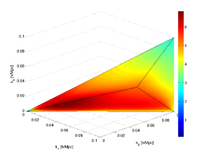
How should we visualize the bispectrum? Fig. 1 shows the leading order matter bispectrum as a three-dimensional color plot. As we shall show in the next section, the leading order matter bispectrum in PT is given by

$$B(k_{1},k_{2},k_{3})=2F_{2}^{(s)}(\textbf{\em k}_{1},\textbf{\em k}_{2})P_{L}(k_{1})P_{L}(k_{2})+(2~{}{\rm cyclic})$$ (2)

where

$$F_{2}^{(s)}(\textbf{\em k}_{1},\textbf{\em k}_{2})=\frac{5}{7}+\frac{\textbf{\em k}_{1}\cdot\textbf{\em k}_{2}}{2}\left(\frac{1}{k_{1}^{2}}+\frac{1}{k_{2}^{2}}\right)+\frac{2}{7}\frac{(\textbf{\em k}_{1}\cdot\textbf{\em k}_{2})^{2}}{k_{1}^{2}k_{2}^{2}},$$ (3)

is the second order PT kernel and $P_{L}(k)$ is the linear matter power spectrum. The three axes of Fig. 1 represent the magnitudes of the three wave numbers, $k_{1}$, $k_{2}$, and $k_{3}$ in which the bispectrum is shown only for the tetrahedronic region defined by $k_{1}\geq k_{2}\geq k_{3}$ and $k_{1}\leq k_{2}+k_{3}$ (trianglular condition). The amplitude of the bispectrum is coded by colors. We can see from Fig 1 that the bispectrum has the largest magnitude at around $k_{1}\simeq k_{2}\simeq k_{3}\sim 0.02~{}h/\mathrm{Mpc}$ where the linear power spectrum peaks. We can also examine the behavior of the bispectrum at the limiting triangular configurations, which are along the planes and lines that make up the shape of the region in which the bispectrum is defined. This way of visualization is often used in the cosmic microwave background (CMB) literature when discussing the bispectrum of temperature anisotropies (Fergusson et al., 2012; Planck Collaboration et al., 2013). While the three-dimensional color plots are useful for showing the overall structure of the bispectrum, it is not apt for showing its detailed shape and scale dependence.

Figure 1: 3-D plot of the full tree-level matter bispectrum, with $k_{1}\geq k_{2}\geq k_{3}$.The color reflects the magnitude of $\log\left(B(k_{1},k_{2},k_{3})\right)$.

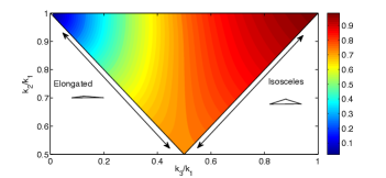
A useful way of visualizing the shape and scale dependence of bispectrum is by plotting slices of constant $k_{1}$. The plots in the left column of Fig 2 show slices of the bispectrum in Fig. 1 at $k_{1}=0.01$ $h$/Mpc, $k_{1}=0.05$ $h$/Mpc, and $k_{1}=0.15$ $h$/Mpc (from top to bottom). Note that the values shown have been normalized by the maximum value of $B(k_{1},k_{2},k_{3})$ in each slice. We also show the locations of the different triangular configurations in the same plot. From these plots, we can see that the squeezed configuration always has a suppressed signal compared to other elongated triangles. On large scales, the bispectrum of equilateral triangles is higher than in other configurations, whereas on smaller scales, it is suppressed compared to, say, isosceles triangles. Jeong & Komatsu (2009) present a detailed discussion about the shape and scale dependence of the leading order matter bispectrum.

(a) $k_{1}=0.01$ h/Mpc

(b) Flattened bispectrum, with $\delta k_{1}=0.001$ h/Mpc

(c) $k_{1}=0.05$ h/Mpc

(d) Flattened bispectrum, with $\delta k_{1}=0.001$ h/Mpc

(e) $k_{1}=0.15$ h/Mpc

(f) flattened bispectrum, with $\delta k_{1}=0.005$ h/Mpc

Figure 2: Left: slices of the bispectrum at constant $k_{1}$. The locations of different triangular configurations are highlighted. Right: the flattened bispectrum with a given $\delta k_{1}$, where the range of $k_{1}$ plotted includes the corresponding slice on the left. Vertical dashed lines indicate different slices of $k_{1}$. Values of $k_{1}$ in several slices is given in units of $h$/Mpc.

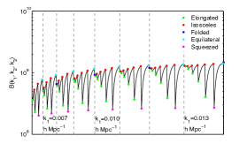
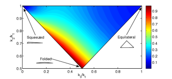
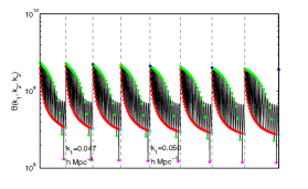
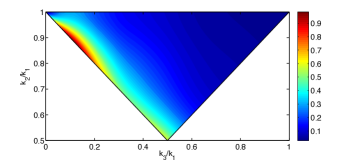
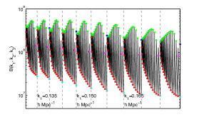
In reality, we can only measure the Fourier space density contrast at discrete grid points whose separation is determined by the volume of the $N$-body simulation, or the width of the survey window function. The bispectrum then can also be measured only for a finite number of triples $(k_{1},k_{2},k_{3})$. We can facilitate the comparison among different predictions for the bispectrum by flattening all possible triplets into a one-dimensional vector ($x$-axis), where we rank the triplet in row-major, ascending order with the condition $k_{1}\geq k_{2}\geq k_{3}$. This allows us to look at all of the triangular configurations over a range of scales simultaneously, as well as compare bispectra on the $y$-axis. Each plot in the right column of Fig. 2 shows the bispectrum of all triangular configurations in a range of $k_{1}$ that includes the slice shown in the left panel. The $x$-axis shows the ranked $(k_{1},k_{2},k_{3})$ triplets, and the $y$-axis shows the amplitude of bispectrum. As one can see from the plots, a similar pattern block is duplicated for each value of the long-wavelength mode $k_{1}$, as indicated by vertical dashed lines. We also show the configuration dependence by highlighting the limiting triangles in different colors. One can easily relate this plot to the contour plot in the left panel. For a given $k_{1}$, the first-ranked triplet is at the bottom vertex ($k_{2}=k_{3}=k_{1}/2$, blue dots, folded triangle) of the triangular region in the left panels ($k_{3}/k_{1}$-$k_{2}/k_{1}$ plane). The rank is followed by the next elongated triangle (green dots) then moves rightward to the isosceles triangles (red dots). This process continues until the rank reaches most-squeezed triplet then walks along the upper-most horizontal line to the equilateral triplet. Depending on the scales ($k_{1}$ values) that we are looking at, the configuration dependence of the bispectrum is different.

In our analysis for this paper, we shall mainly use this flattened representation to study the configuration and scale dependence of bispectrum at all triangles. Although non-linearities change the exact shape of the bispectrum ‘chunk’ for a given $k_{1}$, the overall structure remains unchanged.

3 Transients in Standard Perturbation Theory

In this section, we review the standard perturbation theory (PT) formalism for calculating the tree-level bispectrum (Bernardeau et al., 2002). We then follow the approach of Scoccimarro (1998) and Crocce et al. (2006) to compute the correct growing and decaying modes for initial conditions set using the Zel’dovich Approximation and 2LPT initial conditions.

One way of simplifying the single fluid equations is combining the density field $\delta(\textbf{\em k},\eta)$ and velocity divergence field $\theta(\textbf{\em k},\eta)$ into a doublet as:

$$\Psi_{a}(\textbf{\em k},\eta)=\left(\delta(\textbf{\em k},\eta),-\theta(\textbf{\em k},\eta)/\mathcal{H}\right)\$$ (4)

where the logarithm of the linear growth factor ($D(\tau)$) relative to its initial value ($D_{i}$): $\eta\equiv\ln(D(\tau)/D_{i})\$ is the time variable. Here, $\mathcal{H}\equiv d\ln a/d\tau=aH$ is the reduced Hubble parameter that is defined with conformal time $\tau=\int dt/a(t)$. The equations of motion for $\Psi_{a}$, combining the continuity equation, the Euler equation, and the Poisson equation, can then be written as:

$$\partial_{\eta}\Psi_{a}(\textbf{\em k},\eta) +\Omega_{ab}\Psi_{b}(\textbf{\em k},\eta)$$

$$=\gamma^{(s)}_{abc}(\textbf{\em k},\textbf{\em k}_{1},\textbf{\em k}_{2})\Psi_{b}(\textbf{\em k}_{1},\eta)\Psi_{c}(\textbf{\em k}_{2},\eta).$$ (5)

Here,

$$\Omega_{ab}\equiv\begin{bmatrix}\ 0&-1\ \\ -3/2&1/2\ \end{bmatrix}$$ (6)

is the linear mixing matrix, and

$$\gamma_{121}^{(s)}(\textbf{\em k},\textbf{\em k}_{1},\textbf{\em k}_{2}) =(2\pi)^{3}\delta_{D}(\textbf{\em k}-\textbf{\em k}_{1}-\textbf{\em k}_{2})\frac{\textbf{\em k}\cdot\textbf{\em k}_{1}}{2k_{1}^{2}}$$ (7)

$$\gamma_{222}^{(s)}(\textbf{\em k},\textbf{\em k}_{1},\textbf{\em k}_{2}) =(2\pi)^{3}\delta_{D}(\textbf{\em k}-\textbf{\em k}_{1}-\textbf{\em k}_{2})\frac{k^{2}(\textbf{\em k}_{1}\cdot\textbf{\em k}_{2})}{2k_{1}^{2}k_{2}^{2}}$$ (8)

encode the non-linear interactions. Note that $\gamma_{121}^{(s)}(\textbf{\em k},\textbf{\em k}_{1},\textbf{\em k}_{2})=\gamma_{112}^{(s)}(\textbf{\em k},\textbf{\em k}_{2},\textbf{\em k}_{1})$ and the integration $\int d^{3}k_{i}/(2\pi)^{3}$ over the repeated wavevectors ($\textbf{\em k}_{1}$ and $\textbf{\em k}_{2}$) are implied.

A Laplace transform of Equation (5) in the variable $\eta$ leads to:

$$\omega\Psi_{a}(\textbf{\em k},\omega)-\phi_{a}(\textbf{\em k})+\Omega_{ab}\Psi_{b}(\textbf{\em k},\omega)$$ (9)

$$= \gamma^{(s)}_{abc}(\textbf{\em k},\textbf{\em k}_{1},\textbf{\em k}_{2})\int_{c-i\infty}^{c+i\infty}\frac{d\omega_{1}}{2\pi i}\Psi_{b}(\textbf{\em k}_{1},\omega_{1})\Psi_{c}(\textbf{\em k}_{2},\omega-\omega_{1})\ ,$$

where

$$\phi_{a}(\textbf{\em k})=\Psi_{a}(\textbf{\em k},\eta=0)$$ (10)

is the density and velocity field at the initial time (i.e. the time at which we start the simulation). The linear part of Eq. (9) can be written in terms of a matrix $\sigma_{ab}$:

$$\sigma_{ab}^{-1}(\omega) \equiv\omega\delta_{ab}+\Omega_{ab}$$ (11)

$$\sigma_{ab}(\omega) =\frac{1}{(2\omega+3)(\omega-1)}\begin{bmatrix}2\omega+1&2\ \\ \ 3&2\omega\ \end{bmatrix},$$ (12)

and, finally, we obtain the formal solution through an inverse Laplace transformation as:

$$\Psi_{a}(\textbf{\em k},\eta)=g_{ab}(\eta)\phi_{b}(\textbf{\em k})$$ (13)

$$+\int_{0}^{\eta}d\eta^{\prime}g_{ab}(\eta-\eta^{\prime})\gamma_{bcd}^{(s)}(\textbf{\em k},\textbf{\em k}_{1},\textbf{\em k}_{2})\Psi_{c}(\textbf{\em k}_{1},\eta^{\prime})\Psi_{d}(\textbf{\em k}_{2},\eta^{\prime}).$$

Here,

$$g_{ab}(\eta) =\int_{c-i\infty}^{c+i\infty}\frac{d\omega}{2\pi i}\sigma_{ab}(\omega)e^{\omega\eta}$$ (14)

$$=\frac{e^{\eta}}{5}\begin{bmatrix}3&2\ \\ \ 3&2\ \end{bmatrix}-\frac{e^{-3\eta/2}}{5}\begin{bmatrix}-2&2\ \\ \ 3&-3\ \end{bmatrix}$$

is the Green’s function which describes the time evolution of the linear perturbations. The first term proportional to $e^{\eta}\propto a$ is the growing mode and the second term proportional to $e^{-3\eta/2}\propto a^{-3/2}$ is the decaying mode.

Eq. (13) is the formal solution of the fluid equations, and starting points of various of renormalized perturbation theories. For our purposes, however, it suffices to find the perturbative solution that follows. We perturbatively expand the solutions at initial and final time ($\phi_{a}$ and $\Psi_{a}$, respectively) in terms of the linear (Gaussian) density $\delta_{0}(\textbf{\em k})$ field at initial time as:

$$\phi_{a}(\textbf{\em k}) =\sum_{n=1}^{\infty}\phi_{a}^{(n)}(\textbf{\em k})$$ (15)

$$\Psi_{a}(\textbf{\em k},\eta) =\sum_{n=1}^{\infty}\Psi_{a}^{(n)}(\textbf{\em k},\eta)$$ (16)

where

$$\phi_{a}^{(n)}(\textbf{\em k}) =[\delta_{D}]_{n}\mathcal{T}_{a}^{(n)}(\textbf{\em k}_{1},\cdots,\textbf{\em k}_{n})\delta_{0}(\textbf{\em k}_{1})\cdots\delta_{0}(\textbf{\em k}_{n})$$ (17)

$$\Psi_{a}^{(n)}(\textbf{\em k},\eta) =[\delta_{D}]_{n}\mathcal{F}_{a}^{(n)}(\textbf{\em k}_{1},\cdots,\textbf{\em k}_{n},\eta)\delta_{0}(\textbf{\em k}_{1})\cdots\delta_{0}(\textbf{\em k}_{n})$$ (18)

and $[\delta_{D}]_{n}\equiv\delta_{D}(\textbf{\em k}-\textbf{\em k}_{1}-\cdots-\textbf{\em k}_{n})$. Here, $\mathcal{T}_{a}^{(n)}$ are the $n$-th order kernels of the initial density and velocity fields, and $\mathcal{F}_{a}^{(n)}(\eta)$ are the $n$-th order resulting kernels at a later time $\eta$. Again, the integration $\int d^{3}k_{i}/(2\pi)^{3}$ over the repeated $\textbf{\em k}_{i}$’s is implied. By using this ansatz, we calculate the kernels $\mathcal{F}_{a}^{(n)}$ at the final redshift from the initial kernels $\mathcal{T}_{a}^{(n)}$:

$$\mathcal{F}_{a}^{(n)}(\eta) =g_{ab}(\eta)\mathcal{T}_{b}^{(n)}$$ (19)

$$+\sum_{m=1}^{n-1}\int_{0}^{\eta}ds\ g_{ab}(\eta-s)\gamma_{bcd}^{(s)}\mathcal{F}_{c}^{(m)}(s)\mathcal{F}_{d}^{(n-m)}(s).$$

This recursion relation is the starting point of the transient analysis.

3.1 Growing mode solutions of Standard Perturbation Theory

In the real universe, the decaying modes decay away at very early times, and the density field is at its fastest growing mode for any reasonable choice of the initial redshift. Therefore, the initial conditions for ideal $N$-body simulations must be set at an early enough time such that PT is valid on the smallest resolved scales, and set by the fastest growing modes at all relevant orders in PT.

In this section, we find the fastest growing mode solution perturbatively. We first find the linear growing mode $\phi_{a}^{(1)}(\textbf{\em k})=\delta_{0}(\textbf{\em k})(1,1)$ so that the decaying part of the Green’s function Eq. (14) vanishes. Then, the second order kernels at time $\eta$ are given by Eq. (19) using the linear growing kernel of $\mathcal{F}_{a}^{(1)}=e^{\eta}(1,1)$. While the time integral in Eq. (19) gives rise to the slowly growing mode ($\propto e^{\eta}$) and the decaying mode ($\propto e^{-\frac{3}{2}\eta}$), those are exactly canceled by the initial fastest-growing kernels $\mathcal{T}_{a}^{(2)}=(F_{2}^{(s)},G_{2}^{(s)})$ defined by the kernels in standard PT (Bernardeau et al., 2002) and we are left with the fastest-growing solution of $\mathcal{F}_{2}^{(n)}(\eta)=e^{2\eta}(F_{2}^{(s)},G_{2}^{(s)})$. The same is true for all the higher order kernels, and the fastest growing solutions are

$$\Psi_{a}^{(n)}(\textbf{\em k},\eta)= (2\pi)^{3}\delta_{D}(\textbf{\em k}-\textbf{\em k}_{1}-\cdots-\textbf{\em k}_{n})$$

$$\times\mathcal{F}_{a}^{(n)}(\textbf{\em k}_{1},..,\textbf{\em k}_{n},\eta)\delta_{0}(\textbf{\em k}_{1})\cdots\delta_{0}(\textbf{\em k}_{n}),$$ (20)

where

$$\mathcal{F}_{a}^{(n)}(\eta) =e^{n\eta}\left(F_{n}^{(s)},G_{n}^{(s)}\right)$$ (21)

are the standard PT kernels. In particular, the second order kernel which appears in the leading-order matter bispectrum in Eq. (2) is given by

$$F_{2}^{(s)}(\textbf{\em k}_{1},\textbf{\em k}_{2})=\frac{5}{7}+\frac{\textbf{\em k}_{1}\cdot\textbf{\em k}_{2}}{2}\left(\frac{1}{k_{1}^{2}}+\frac{1}{k_{2}^{2}}\right)+\frac{2}{7}\frac{(\textbf{\em k}_{1}\cdot\textbf{\em k}_{2})^{2}}{k_{1}^{2}k_{2}^{2}},$$ (22)

and the velocity kernel is given by

$$G_{2}^{(s)}(\textbf{\em k}_{1},\textbf{\em k}_{2})=\frac{3}{7}+\frac{\textbf{\em k}_{1}\cdot\textbf{\em k}_{2}}{2}\left(\frac{1}{k_{1}^{2}}+\frac{1}{k_{2}^{2}}\right)+\frac{4}{7}\frac{(\textbf{\em k}_{1}\cdot\textbf{\em k}_{2})^{2}}{k_{1}^{2}k_{2}^{2}}.$$ (23)

When the single fluid approximation is valid (at early times and on large scales), ideal $N$-body simulations must reproduce the density and velocity fields in Eq. (20) with the growing mode kernels Eq. (21). To satisfy this condition, we must start simulations with initial density and velocity fields satisfying Eq. (20).

3.2 Transients from Initial conditions of $N$-body simulations

Generating the fastest-growing initial conditions at all orders in perturbation theory is quite non-trivial. This is in part because we simulate $N$-body dynamics with the motion of matter particles. That is, the initial conditions for $N$-body simulations are set by position and velocity of each particle (rather than set by density and velocity gradient field as is demanded by the PT analysis). Due to the nonlinear relation between particle’s position and the resulting density field, the initial conditions can only satisfy the fastest-growing condition perturbatively, in an order-by-order manner. As a result, when generating initial conditions with the growing mode at a given order in $\delta_{0}$, it is inevitable that spurious decaying modes will be excited at higher orders.

In this section, we study the decaying modes for two of the most widely used initial condition generators: first order (Zel’dovich approximation) and second order (2LPT) Lagrangian perturbation theory (LPT). For each initial condition generating scheme, we calculate the initial density and velocity kernels $\mathcal{T}_{a}^{(n)}$, and find the evolved kernel at the final redshift by using Eq. (19) in order to study the resulting transients in the matter bispectrum as a function of initial and final redshifts as well as triangular configuration and scales.

LPT describes the evolution of the matter density field by displacement $\mathbf{\Psi}$ between each matter particle’s initial Lagrantian position q and final position x:

$$\textbf{\em x}(\textbf{\em q},\eta)=\textbf{\em q}+\mathbf{\Psi}(\textbf{\em q},\eta),$$ (24)

then the peculiar velocity field is given by

$$\textbf{\em v}(\textbf{\em q},\eta)=\frac{d\textbf{\em x}}{d\tau}\equiv\mathbf{\Psi}^{\prime}(\textbf{\em q},\eta).$$ (25)

Note that x is the comoving coordinate, and prime denotes the time derivative with respect to the conformal time $\tau$. When it comes to generating initial conditions of $N$-body simulations, q refers to the position of particles on a regular grid, and x refers to particle’s initial position.

For a given displacement field $\mathbf{\Psi}$, we find the Fourier space density contrast and velocity gradient in terms of the displacement field as

$$\delta(\textbf{\em k},\eta)= \int d^{3}\textbf{\em x}\,\delta(\textbf{\em x})e^{-i\textbf{\em k}\cdot\textbf{\em x}}$$

$$= \sum_{n=1}\frac{1}{n!}\int d^{3}qe^{-i\textbf{\em k}\cdot\textbf{\em q}}\left[-i\textbf{\em k}\cdot\mathbf{\Psi}(\textbf{\em q},\eta)\right]^{n},$$ (26)

$$\theta(\textbf{\em k},\eta)= \int d^{3}qJ(\textbf{\em q},\eta)\nabla_{x}\cdot\mathbf{\Psi}^{\prime}(\textbf{\em q},\eta)e^{-i\textbf{\em k}\cdot(\textbf{\em q}+\mathbf{\Psi}(\textbf{\em q},\eta))},$$ (27)

where we calculate the Jacobian $J(\textbf{\em q},\eta)$ by using mass conservation $J(\textbf{\em q},\eta)=\left|\partial^{3}x/\partial^{3}q\right|=\left(1+\delta(\textbf{\em x})\right)^{-1}=|\delta_{ij}+\mathbf{\Psi}_{i,j}|$. Here, comma stands for the derivative with respect to the Lagrangian coordinate. As the cosmic matter field on large scales is irrotational, we introduce the scalar potential such that $\Psi_{i}=-\phi_{,i}$. In $n$-th order LPT, the scalar potential $\phi$ is expanded up to $n$-th order in the linear density contrast $\delta_{0}(\textbf{\em k})$ (Bouchet et al., 1995).

3.2.1 Zel’dovich approximation

In the Zel’dovich approximation, the scalar potential $\phi$ is given by

$$\phi(\textbf{\em k})=-\frac{1}{k^{2}}\delta_{0}(\textbf{\em k}),$$ (28)

and from Eqs. (26)–(27) we find the linear order initial kernels is

$$\mathcal{T}_{a}^{\mathrm{ZA},(1)}=(1,1).$$ (29)

This means the Zel’dovich approximation indeed gives rise to the growing mode solution in linear order. On the other hand, the second order initial kernels are

$$\mathcal{T}_{a}^{\mathrm{ZA},(2)}=\left(\frac{(\textbf{\em k}\cdot\textbf{\em k}_{1})(\textbf{\em k}\cdot\textbf{\em k}_{2})}{2k_{1}^{2}k_{2}^{2}},~{}\frac{k^{2}(\textbf{\em k}_{1}\cdot\textbf{\em k}_{2})}{2k_{1}^{2}k_{2}^{2}}\right),$$ (30)

which are different from the fastest-growing mode kernels of PT in Eq. (21). Therefore, the transients in the Zeld’ovich approximation start to appear from second order, and affect the subsequent evolution of the density and velocity fields at second order as

$$F_{2}^{\mathrm{ZA},(2)}(\textbf{\em k}_{1},\textbf{\em k}_{2},\eta)=e^{2\eta}F_{2}^{(s)}(\textbf{\em k}_{1},\textbf{\em k}_{2},\eta)$$

$$\qquad+\left(\hat{t}_{ij}(\textbf{\em k}_{1})\hat{t}_{ij}(\textbf{\em k}_{2})-\frac{2}{3}\right)\left(\frac{3}{10}e^{\eta}-\frac{3}{35}e^{-\frac{3}{2}\eta}\right)$$ (31)

$$G_{2}^{\mathrm{ZA},(2)}(\textbf{\em k}_{1},\textbf{\em k}_{2},\eta)=e^{2\eta}G_{2}^{(s)}(\textbf{\em k}_{1},\textbf{\em k}_{2},\eta)$$

$$\qquad+\left(\hat{t}_{ij}(\textbf{\em k}_{1})\hat{t}_{ij}(\textbf{\em k}_{2})-\frac{2}{3}\right)\left(\frac{3}{10}e^{\eta}+\frac{9}{70}e^{-\frac{3}{2}\eta}\right).$$ (32)

Here, $\hat{t}_{ij}(\textbf{\em k})$ is the longitudinal operator which relates the density field and the tidal field $s_{ij}(\textbf{\em k})$

$$s_{ij}(\textbf{\em k})=\left[\frac{k_{i}k_{j}}{k^{2}}-\frac{\delta_{ij}}{3}\right]\delta(\textbf{\em k})\equiv\hat{t}_{ij}(\textbf{\em k})\delta(\textbf{\em k}),$$ (33)

which means that the Zel’dovich approximation contributes an extra tidal field to the $N$-body simulation at second order.

The extra tidal field then yields a transient in the leading order matter bispectrum, and the slowest-decaying transient is given by

$$B^{\mathrm{ZA}}(k_{1},k_{2},k_{3})-B(k_{1},k_{2},k_{3})$$

$$= \frac{3}{5}\left[\frac{D}{D_{i}}\right]^{3}\left(\mu_{12}^{2}-1\right)P_{L}(k_{1})P_{L}(k_{2})+(2~{}\mathrm{cyclic}),$$ (34)

with $\mu_{ij}=\hat{\textbf{\em k}}_{i}\cdot\hat{\textbf{\em k}}_{j}$ being the angular cosine between two wave vectors. With Eq. (19), one can also show that, with Zel’dovich initial conditions, the slowest-decaying (or, longest-lasting) transients at all higher orders ($n\geq 2$) are suppressed only by $e^{\eta}$ with respect to the fastest-growing modes.

3.2.2 2LPT

In 2LPT, the scalar potential is given by

$$\phi(\textbf{\em k})=\frac{\delta_{0}(\textbf{\em k})}{k^{2}}+(2\pi)^{3}\delta^{D}(\textbf{\em k}-\textbf{\em k}_{12})\frac{3(1-\mu_{12}^{2})}{14k^{2}}\delta_{0}(\textbf{\em k}_{1})\delta_{0}(\textbf{\em k}_{2}),$$ (35)

with $\textbf{\em k}_{12}=\textbf{\em k}_{1}+\textbf{\em k}_{2}$, which reads, from Eqs. (26)–(27),

$$\mathcal{T}_{a}^{\mathrm{2LPT},(1)}= \ (1,1)$$ (36)

$$\mathcal{T}_{a}^{\mathrm{2LPT},(2)}= \ (F_{2}^{(s)},G_{2}^{(s)}).$$ (37)

Then, as shown in Sec. 3.1, the density and velocity fields in 2LPT remain as the fastest-growing modes, and an $N$-body simulation with 2LPT initial conditions correctly reproduces the leading order bispectrum.

On the other hand, 2LPT initial conditions differ from the fastest-growing modes at third order. This generates spurious slowly growing modes and decaying modes. Again, using Eq. (19), one can show that, for 2LPT initial conditions, the slowest-decaying modes are suppressed by two powers in the linear growth factor ($e^{-2\eta}$) with respect to the fastest growing mode at $n(\geq 3)$-th order. Therefore, we expect the following time dependence of transient:

$$B^{\mathrm{2LPT}}(k_{1},k_{2},k_{3})-B(k_{1},k_{2},k_{3})\propto\left[\frac{D}{D_{i}}\right]^{2},$$ (38)

and to contribute on smaller scales than the Zel’dovich case because the transient only comes from next-to-leading order and beyond. Relative to the leading-order, fastest growing mode, the transient decays faster than the Zel’dovich case as $(D/D_{i})^{-2}$.

4 Transients in Simulations

In this section, we study the error induced by transients numerically with a suite of simulations with different initial redshifts, using both the Zel’dovich approximation (ZA) and 2LPT for setting the initial positions and velocities of particles.

We examine a set of twelve simulations with different initial redshifts, but with the same random seed to set initial conditions. This ensures that within each set, any differences we measure between the simulations are due solely to the initial conditions generator. The initial conditions in six of the runs were generated using ZA, and in the other six we used 2LPT. We use the following initial redshifts in each case: $z_{\rm init}=400,300,200,100,50,25$. We use the 2LPT simulation started at $z_{\rm init}=400$ as our reference simulation to which all other runs are compared. That is, this simulation defines our fiducial statistics, $P^{\mathrm{fid}}$ and $B^{\mathrm{fid}}$.

We run the simulations using the TreePM part of the publicly available version of Gadget 2 code. Each simulation is run with $512^{3}$ particles in a 200 Mpc/$h$ box and particle-mesh Fourier grid $N_{\rm grid}=1024^{3}$. The background universe is $\Lambda$CDM with the following cosmological parameters ($\Omega_{\Lambda}=0.73$, $\Omega_{m}=0.27$, $h=0.7$), and the initial density field is calculated from the primordial curvature power spectrum with spectral index $n_{s}=0.96$, and normalized so that the r.m.s. fluctuation smoothed by a spherical top-hat filter with radius $8~{}\rm{Mpc}/h$ is $\sigma_{8}=0.8$ at present ($z=0$). To minimize the effect from accumulated numerical noise, we have required stringent accuracy of N-body simulation by setting parameters of Gadget 2 following the choice of Crocce et al. (2006): ErrTolIntAccuracy = 0.01, MaxRMSDisplacementFac = 0.1, MaxSizeTimestep = 0.01, ErrTolTheta = 0.2, ErrTolForceAcc = 0.002. We calculate the cloud-in-cell density from the output particle distribution on a $1024^{3}$ grid at $z=6,5,4,3,2$ and $1$ and compute the power spectrum and bispectrum at each redshift.

4.1 Transients in the matter power spectrum

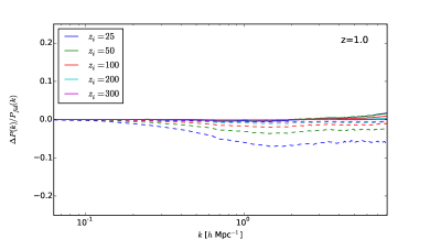
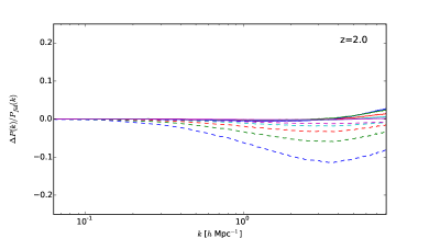
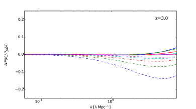
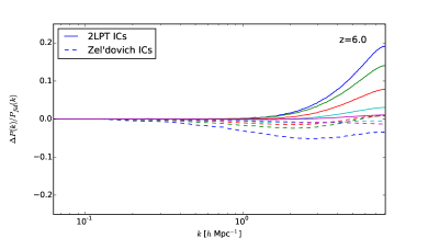
Figure 3 shows the fractional error in the measured power spectrum, as compared to the fiducial power spectrum, at $z=1,2,3$, and $6$, from 2LPT (solid) and ZA (dashed) initial conditions. The various initial redshifts are shown in different colors. As expected, the transients from ZA initial conditions are in general larger than 2LPT on all scales and redshifts, apart from on very small scales at $z=6$, and the error is larger for smaller initial redshifts in all cases. While the 2LPT power spectrum transients decay quickly, the ZA transients remain significant, even on relatively large scales, until $z=1$. These findings are consistent with PT predictions for transients in the matter power spectrum, and also with previous studies Crocce et al. (2006); Jeong (2010).

(a) Transient effect at $z=1$

(b) Transient effect at $z=2$

(c) Transient effect at $z=3$

(d) Transient effect at $z=6$

Figure 3: Error induced by transients in the measured power spectrum at redshifts $z=1,2,3,6$ using Zel’dovich and 2LPT initial conditions with different initial redshifts. In each plot, the left column shows the results from the large-box simulation and the right column shows the small-box simulation. The top panels of the plots show the error in simulations using 2LPT initial conditions and the bottom panels show the error from Zel’dovich initial conditions.

4.2 Transients in the matter bispectrum

(a) Transient effect at $z=1$

(b) Transient effect at $z=2$

(c) Transient effect at $z=3$

(d) Transient effect at $z=6$

Figure 4: Error induced by transients in the measured bispectrum at redshifts $z=1,2,3,6$ using Zel’dovich and 2LPT initial conditions with different initial redshifts. The top panels of the plots show the error in simulations using 2LPT initial conditions at various initial redshifts and the bottom panels show the error from Zel’dovich initial conditions. The different line colors indicate different initial redshifts for the simulations. Vertical dashed lines indicate slices of $k_{1}$, and the $k_{1}$ values of several slices are indicated along the $x$-axis in units of $h$/Mpc.

(a) Transient effect at $z=1$

(b) Transient effect at $z=2$

(c) Transient effect at $z=3$

(d) Transient effect at $z=6$

Figure 5: Same as Figure 4, but for the reduced bispectrum, $Q$.

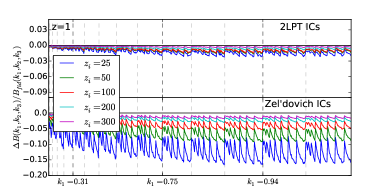
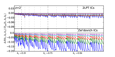
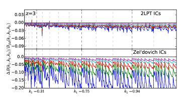
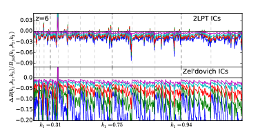
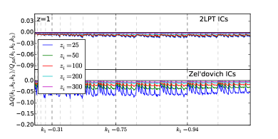
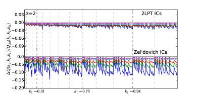
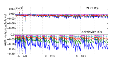
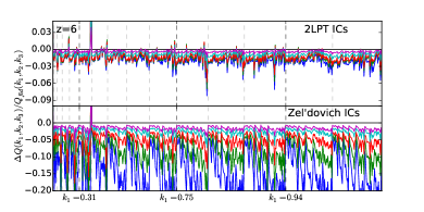
Figure 4 shows the fractional error in the measured bispectrum compared to the fiducial bispectrum, again at $z=1,2,3$, and $6$, from 2LPT (top) and ZA (bottom) initial conditions. Note the different $y$-ranges in the two panels. As we found with the power spectrum transients, the error is larger for smaller initial redshifts. The bispectrum transient error from the ZA simulations is significantly larger on all scales than in the 2LPT simulations, because the ZA transients appear at tree-level as opposed to 1-loop in PT. We also note that the transient error is larger at higher redshift in all cases, as expected from theory. We also show the transient effect in the corresponding reduced bispectrum

$$Q(k_{1},k_{2},k_{3})=\frac{B(k_{1},k_{2},k_{3})}{P(k_{1})P(k_{2})+P(k_{2})P(k_{3})+P(k_{3})P(k_{1})}$$ (39)

in Figure 5. As expected, when removing the effects due to the transients in the power spectrum, the transient effects in the reduced bispectrum are smaller, in particular for lower redshifts and smaller scales, than the transients in the bispectrum. The transients in 2LPT simulations, however, are much smaller than those in ZA simulations.

In order to accurately model the nonlinear bispectrum numerically, we suggest using 2LPT initial conditions with an initial redshift $z_{\rm init}\geq 100$. For $z_{i}=100$, the error from transients is less than 1% for $z\leq 3$ and around $2$% at $z=6$ for this box size and resolution. For the corresponding ZA simulation, the errors are around 8% for $z\leq 3$ and 10% for $z=6$. Although the degree of the transient effect depends on other factors such as the resolutions of simulation, we find this rule of thumb also works for simulations with $L_{\rm box}=1~{}{\rm Gpc}/h$ and $N_{\rm particle}=512^{3}$.

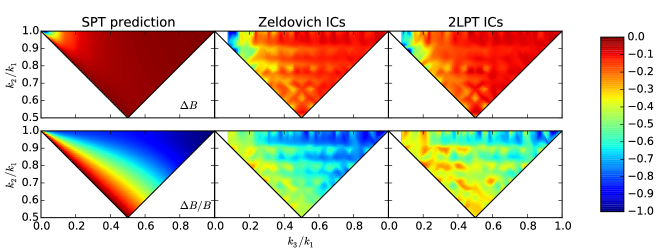
Another consideration is the shape-dependence of the bispectrum transients. Figure 6 shows the transient signal ($\Delta B=B-B^{\mathrm{fid}}$; top) and induced error ($\Delta B/B^{\mathrm{fid}}$; bottom) at $k_{1}=0.7$ $h$/Mpc (normalized to $-1$). On the left is the prediction from PT for the transients from ZA initial conditions. The middle column shows the signal and error measured from the the $z_{i}=200$ ZA simulation at $z=1$. The right column shows the same for the 2LPT simulation with $z_{i}=200$.

While Figure 4 clearly shows that the 2LPT transients have a much smaller amplitude than the ZA transients, Figure 6 shows that they have very similar shape-dependence to ZA transients on these scales. The measured shape dependences of the transient signal (top panels) and error (bottom panels) agree reasonably well with the SPT prediction for both ZA and 2LPT ICs. The error induced from transients is greatest in the equilateral configuration, and smallest in the elongated configuration for both ZA and 2LPT initial conditions. We find that the shape dependence of the transients is independent of redshift in both ZA and 2LPT cases; it is only the amplitude of transients that is reduced at lower redhsifts because the decaying modes fade out as the simulation proceeds.

Figure 6: Shape dependence of the transient signal and error in the measured bispectrum at $k_{1}=0.7$ $h$/Mpc at $z=1$ from Zel’dovich and 2LPT initial conditions compared to the SPT prediction. The top panels show the transient signal, which is highest in the squeezed and elongated configurations. The bottom panels show the percent error induced by transients, which is highest in the equilateral configuration. Each slice is normalized by its minimum value, so the range is from $-1$ to $0$ in each case.

5 Modeling Nonlinearity in the matter bispectrum

We now test the accuracy of various theoretical templates for the nonlinear bispectrum against the measured matter bispectrum from $N$-body simulations. For comparison, we use the result of $z_{\rm init}=400$ (2LPT) simulation, as the nonlinear matter bispectra measured from other 2LPT simulations converge to it.

On large enough scales, the leading order (tree level) prediction in Eq. (2) is enough to model the matter bispectrum. Modeling the matter bispectrum on smaller scales where nonlinearities become stronger, however, requires more elaborate calculation. On quasi-linear scales, we expect the next-to-leading order (one-loop) bispectrum in PT to model the nonlinear evolution reasonably well. The next-to-leading order matter bispectrum is given by four additional one-loop terms (Bernardeau et al., 2002):

$$B^{\rm 1loop}(k_{1},k_{2},k_{3})= B^{\rm tree}(k_{1},k_{2},k_{3})+B^{(222)}(k_{1},k_{2},k_{3})$$

$$+ B^{(123a)}(k_{1},k_{2},k_{3})+B^{(123b)}(k_{1},k_{2},k_{3})$$

$$+ B^{(114)}(k_{1},k_{2},k_{3}),$$ (40)

where $B^{\rm tree}$ is the leading order bispectrum in Eq. (2) and

$$B^{(222)}(k_{1},k_{2},k_{3})=8\int\frac{d^{3}q}{(2\pi)^{3}}F_{2}^{(s)}(\textbf{\em q},\textbf{\em k}_{1}-\textbf{\em q})$$

$$\times F_{2}^{(s)}(-\textbf{\em q},\textbf{\em k}_{2}+\textbf{\em q})F_{2}^{(s)}(\textbf{\em q}-\textbf{\em k}_{1},-\textbf{\em k}_{2}-\textbf{\em q})$$

$$\times P_{L}(q)P_{L}(|\textbf{\em k}_{1}-\textbf{\em q}|)P_{L}(|\textbf{\em k}_{2}+\textbf{\em q}|)$$ (41)

$$B^{(114)}(k_{1},k_{2},k_{3})=12P_{L}(k_{2})P_{L}(k_{3})\int\frac{d^{3}q}{(2\pi)^{3}}P_{L}(q)$$

$$\times F_{4}^{(s)}(\textbf{\em q},-\textbf{\em q},-\textbf{\em k}_{2},-\textbf{\em k}_{3})+(2~{}\mathrm{cyc.})$$ (42)

$$B^{(123a)}(k_{1},k_{2},k_{3})=6P_{L}(k_{1})\int\frac{d^{3}q}{(2\pi)^{3}}P_{L}(q)P_{L}(|\textbf{\em k}_{2}-\textbf{\em q}|)$$

$$\times F_{2}^{(s)}(\textbf{\em q},\textbf{\em k}_{2}-\textbf{\em q})F_{3}^{(s)}(-\textbf{\em q},\textbf{\em q}-\textbf{\em k}_{2},-\textbf{\em k}_{1})+(5~{}\mathrm{cyc.})$$ (43)

$$B^{(123b)}(k_{1},k_{2},k_{3})=6P_{L}(k_{1})P_{L}(k_{3})F_{2}^{(s)}(\textbf{\em k}_{1},\textbf{\em k}_{3})$$

$$\times\int\frac{d^{3}q}{(2\pi)^{3}}F_{3}^{(s)}(\textbf{\em q},-\textbf{\em q},\textbf{\em k}_{3})P_{L}(q)+(5~{}\mathrm{cyc.}),$$ (44)

are non-linear corrections with $F_{n}^{(s)}$ being symmetric kernels encoding the fastest growing mode of the nonlinear density evolution (see, e.g. Sec. 3). Note that the expression above is completely determined by the given linear matter power spectrum $P_{L}(k)$.

On smaller scales where PT breaks down due to strong nonlinearities, various phenomenological models have been proposed as alternative ways of predicting the nonlinear behavior of the matter bispectrum. Here, we consider three such models (PT+, GM model Gil-Marín et al. (2012), and SC model Scoccimarro & Couchman (2001), see below for details) for the nonlinear matter bispectrum.

The simplest model that we consider is PT+, where we attribute the entirety of the nonlinear evolution of the matter bispectrum to the nonlinear matter power spectrum. This leads to an expression that is identical to Eq. (2), but uses the measured (fully-nonlinear) power spectrum from the $N$-body simulation in place of the linear power spectrum:

$$B(k_{1},k_{2},k_{3}) =2F_{2}^{(s)}(\textbf{\em k}_{1},\textbf{\em k}_{2})P(k_{1})P(k_{2})+\text{(2 cyc.)}$$ (45)

This model is motivated from the expression of the one-loop bispectrum in Eq. (40), which can be written as $B^{\rm 1loop}(k_{1},k_{2},k_{3})=2F_{2}^{(s)}(\textbf{\em k}_{1},\textbf{\em k}_{2})P_{\rm 1loop}(k_{1})P_{\rm 1loop}(k_{2})+2\mathrm{(cyc.)}+$(irreducible terms), with the one-loop power spectrum $P_{\rm 1loop}(k)$. In the language of renormalized perturbation theory Crocce & Scoccimarro (2006), PT+ corresponds to fixing the ‘vertex’ (the kernel $F_{2}^{(s)}$) while using the renormalized propagator (power spectrum $P(k)$).

PT+ is a simplified version of the fitting formula proposed by Scoccimarro & Couchman (2001) (hereafter, SC), where the $F_{2}^{(s)}$ kernel in Eq. (45) is replaced by the effective kernel $F_{2}^{\rm eff}$ as follows.

$$F_{2}^{\text{\rm eff}}(\textbf{\em k}_{i},\textbf{\em k}_{j}) =\frac{5}{7}a(n_{i},k_{i})a(n_{j},k_{j})$$

$$\qquad+\frac{1}{2}\cos(\theta_{ij})\left(\frac{k_{i}}{k_{j}}+\frac{k_{j}}{k_{i}}\right)b(n_{i},k_{i})b(n_{j},k_{j})$$

$$\qquad+\frac{2}{7}\cos^{2}(\theta_{ij})c(n_{i},k_{i})c(n_{j},k_{j}).$$ (46)

Here, $\theta_{ij}$ is the angle between two wavevectors $\textbf{\em k}_{i}$ and $\textbf{\em k}_{j}$, and $F_{2}^{\rm eff}$ reduces to the PT kernel in Eq. (22) when $a=b=c=1$. The three functions $a(n,k)$, $b(n,k)$, $c(n,k)$ are given as functions of the wavenumber $k$ and the effective slope of the linear power spectrum $n\equiv d\ln P_{L}(k)/d\ln k$ as

$$a(n,k) =\frac{1+\sigma_{8}^{a_{6}}(z)[0.7Q_{3}(n)]^{1/2}(qa_{1})^{n+a_{2}}}{1+(qa_{1})^{n+a_{2}}}$$ (47)

$$b(n,k) =\frac{1+0.2a_{3}(n+3)q^{n+3}}{1+q^{n+3.5}}$$ (48)

$$c(n,k) =\frac{1+4.5a_{4}/[1.5+(n+3)^{4}](qa_{5})^{n+3}}{1+(qa_{5})^{n+3.5}},$$ (49)

where $q\equiv k/k_{\rm nl}$ with nonlinear scale $k_{\rm nl}$ defined by the wavenumber at which the dimensionless power spectrum $\Delta^{2}(k)\equiv k^{3}P_{L}(k)/(2\pi^{2})$ becomes unity $\Delta^{2}(k_{\mathrm{nl}})\equiv 1$, and varies with redshift as $k_{\mathrm{nl}}\propto(1+z)$. $Q_{3}(n)\equiv(4-2^{n})/(1+2^{n+1})$. SC fit the parameters $a_{1}$ through $a_{6}$ using the bispectrum measured from $\mathrm{P^{3}M}$ simulations Jenkins et al. (1998) with $256^{3}$ particles in a $240~{}\mathrm{Mpc}/h$ box to find that $a_{1}=0.25$, $a_{2}=3.5$, $a_{3}=2$, $a_{4}=1$, $a_{5}=2$, $a_{6}=-0.2$.

Recently, Gil-Marín et al. (2012) (hereafter, GM) proposed extending the SC model further with $3$ additional parameters, where $a(n,k)$, $b(n,k)$ and $c(n,k)$ in the effective kernel $F_{2}^{\rm eff}$ are replaced by tilded functions as

$$\tilde{a}(n,k) =\frac{1+\sigma_{8}^{a_{6}}(z)[0.7Q_{3}(n)]^{1/2}(qa_{1})^{n+a_{2}}}{1+(qa_{1})^{n+a_{2}}}$$ (50)

$$\tilde{b}(n,k) =\frac{1+0.2a_{3}(n+3)q^{n+3}(qa_{7})^{n+3+a_{8}}}{1+(qa_{7})^{n+3.5+a_{8}}}$$ (51)

$$\tilde{c}(n,k) =\frac{1+4.5a_{4}/[1.5+(n+3)^{4}](qa_{5})^{n+3+a_{9}}}{1+(qa_{5})^{n+3.5+a_{9}}}.$$ (52)

The definitions for $n$, $q$, $k_{\text{nl}}$, and $Q_{3}$ are the same as above, except in this model $n(k)$ is smoothed so the oscillatory features from the Baryon Acoustic Oscillations (BAO) are removed (further discussion of this can be found in Gil-Marín et al. (2012)). Then, GM fit the parameters $a_{1}$ to $a_{9}$ using the measured matter bispectrum from two sets of $N$-body simulations, one with $L=2.4$ Gpc/$h$ ($768^{3}$ particles), and one with $L_{b}=1.875$ Gpc/$h$ ($1024^{3}$ particles), to find the best-fit parameters of $a_{1}=0.484$, $a_{2}=3.740$, $a_{3}=-0.849$, $a_{4}=0.392$, $a_{5}=1.013$, $a_{6}=-0.575$, $a_{7}=0.128$, $a_{8}=-0.722$, $a_{9}=-0.926$.

Note that the conditions on which the fitting formulae are developed are quite different. While SC have used the matter bispectrum at all triangular configurations (a total of a million triangles for $k\lesssim 2.3$ $h$/Mpc) at redshift $z=0$ and $z=1$, GM have only used certain configurations ($\theta_{12}/\pi=0.1$, $0.2$, $\cdots$, $0.9$ and $k_{2}/k_{1}=1.0$, $1.5$, $2.0$, $2.5$, for $k_{2}<0.4$ Mpc/$h$) at four different redshifts $z=0$, $0.5$, $1$, $1.5$. Moreover, they are subject to different levels of transient errors as the $\Lambda$CDM simulations used by SC are generated at $z_{\rm init}=30$ with the Zel’dovich approximation, and the simulations used by GM are generated by 2LPT at $z_{\rm init}=19$ ($2.4$ Gpc/$h$ box) and $z_{\rm init}=49$ ($1.875$ Gpc/$h$ box).

Figure 7: The bispectrum at $z=0$ measured from the 1 Gpc/$h$ simulation, compared to the SC (green), GM (blue), PT (grey), and PT+ (red) models. The top plot shows the full flattened bispectrum, and the bottom plot shows only the squeezed and equilateral triangles as a function of $k_{1}$.

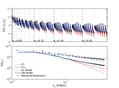
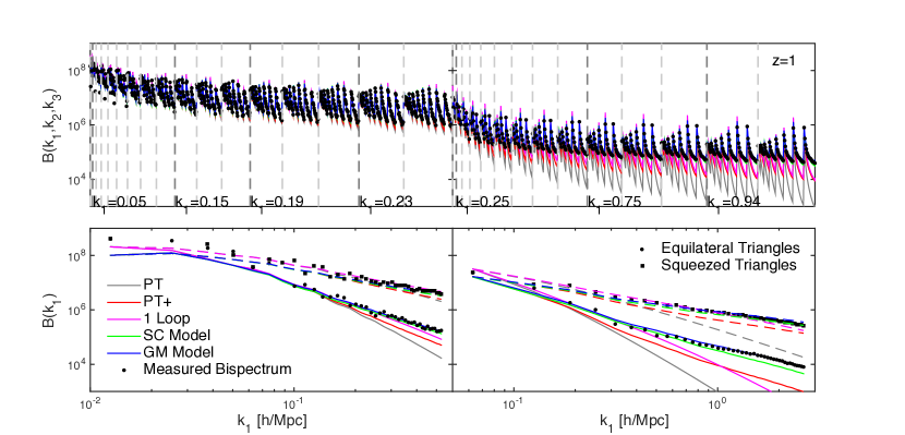
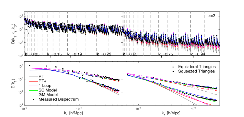
To test the validity of each of the phenomenological formulae outside of the dynamical (Fourier) ranges and redshift ranges at which the models are fitted for, we compare the model predictions to measured bispectra at redshifts $1<z<6$ in both large-scale ($L_{\text{box}}=1$ Gpc/$h$) and small-scale ($L_{\text{box}}=200$ Mpc/$h$) simulations. We also compare these to the predictions from tree-level PT, PT+, and 1-loop PT. For both the SC and GM models, we calculate the effective slope of the linear power spectrum $n(k)$ from the BAO-smoothed linear power spectrum which provides better agreement than the $n(k)$ including BAO.

Figure 8: The bispectrum at $z=1$ measured from the large-box (left) and small-box (right) simulations, compared to the SC (green), GM (blue), PT (grey), and PT+ (red) models. The top plot shows the full flattened bispectrum, and the bottom plot shows only the squeezed and equilateral triangles as a function of $k_{1}$.

First, we check that we can reproduce the results from Gil-Marín et al. (2012) at $z=0$ on large scales. We expect that the GM model is the most accurate here, because their model parameters were fit from a similar simulation. Figure 7 shows the measured bispectrum at $z=0$ from the 1 Gpc/$h$ simulation, compared to the SC and GM models, as well as PT and PT+. The top plot shows the full flattened bispectrum, and the bottom plot shows only the squeezed and equilateral triangles as a function of $k_{1}$. We can see that the GM model indeed gives an improved agreement to the measured bispectrum over the SC model on these scales at $z=0$.

Figure 9: Same as Fig. 8 but for $z=2$.

Next we look at $z=1$ in both the 1 Gpc/$h$ and 200 Mpc/$h$ simulations. Figure 8 compares the measured bispectrum to the models at $z=1$. The left column shows the results from the large-box simulation, and the right shows the small-box simulation. Note that the $k_{1}$ range in the bottom plots overlaps, but we plot the results from the two simulations separately for clarity. Also note that the measured signal for squeezed triangles from the two simulations is slightly different due to the different resolutions. From these plots, we see that the GM model still gives the best fit to the measured bispectrum on the scales shown in all triangular configurations, except for squeezed triangles on very small scales, where the SC model fits slightly better.

Figure 10: Same as Fig. 8 but for $z=3$.

Figure 11: Same as Fig. 8 but for $z=6$.

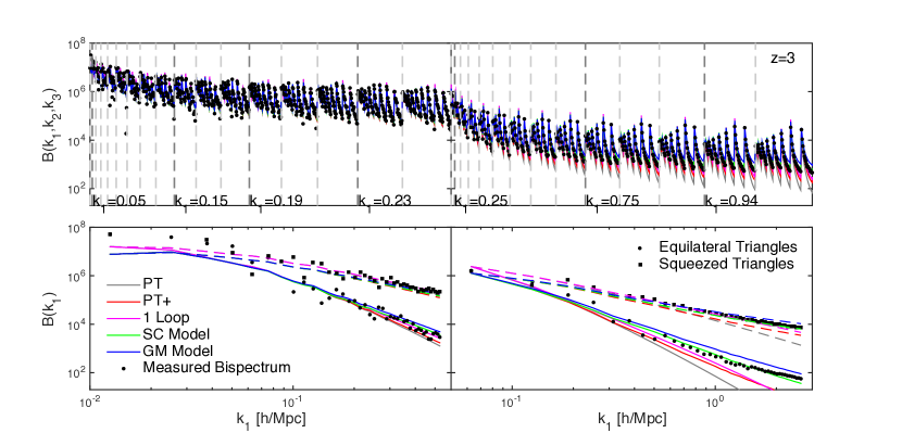
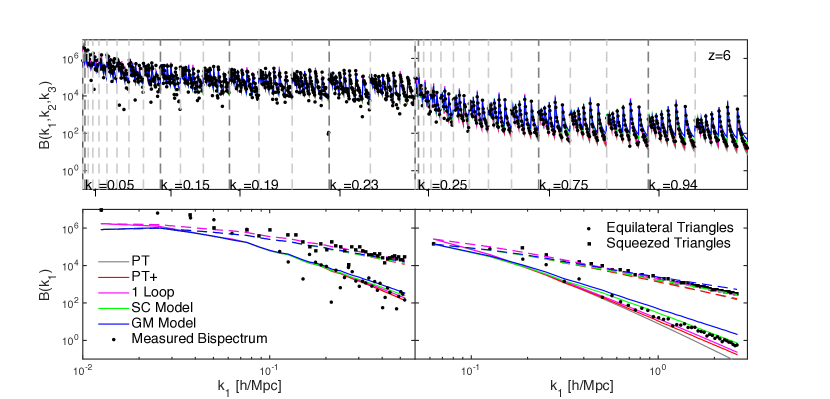
However, we find at higher redshifts, the GM model is less accurate than the SC model. Figs. 9, 10, and 11 show the measured bispectrum at $z=2$, $3$, and $6$, respectively, from both simulations compared to the models. In all of these cases, the SC model gives the most accurate prediction on all scales and in all triangular configurations. The GM model over-predicts the bispectrum slightly in all cases. On large scales (left panels), the predictions from perturbation theory (1-loop and PT+) give reasonably accurate predictions.

It is clear from these comparisons that one must carefully consider the range of validity of a given model when predicting the nonlinear bispectrum. At $z\leq 1$, the GM model undoubtedly gives the best prediction, but at higher redshifts, it is better to use the SC model. At high redshift ($z\geq 3$), the PT models are sufficient for modeling the nonlinear bispectrum. Further work is needed to develop a more reliable model of the nonlinear bispectrum on all scales and redshifts.

6 Conclusion

As the non-linear growth of structure generally causes the cosmic density field to become non-Gaussian, studying higher-order statistics beyond the two-point correlation function will open up a new avenue to exploit a wealth of cosmological information. In particular, with a large-volume coverage and high number density of galaxies, current and future galaxy surveys promise ever-more accurate measurements of the galaxy three-point function and bispectrum. These measurements of three-point correlation functions can give us a better understanding of the growth of structure, galaxy bias, and primordial non-Gaussianity.

Extracting information from the galaxy bispectrum requires accurate modeling of the bispectrum of the dark-matter density field. We have shown that when studying the matter bispectrum numerically, it is important to understand the effects of transients from initial conditions in simulations. When generating the initial conditions using Zel’dovich approximation, the transient of the matter bispectrum shows up at leading order in perturbation theory and affects all scales. In contrast, the transient of the matter power spectrum shows up only at higher-order and affects mainly small scales. In order to simulate nonlinearity in the matter bispectrum correctly, a 2LPT (second-order Lagrangian perturbation theory) initial conditions generator must be used. To further reduce the effects of higher-order transients, we recommend using 2LPT initial conditions with $z_{\text{init}}>100$. This requirement is based on our suite of simulations, in order to maintain a sub-percent level accuracy of the matter bispectrum on scales $k<1\ h$/Mpc at $z\leq 3$.

Another challenge is theoretical modeling of the nonlinear behavior of the bispectrum beyond tree-level perturbation theory. We have shown that analytical calculations of the next-to-leading order, one-loop bispectrum models the non-linearities in the matter bispectrum quite well on quasi-nonlinear scales, in particular at high redshifts. The fact that this analytical calculation of the one-loop bispectrum, which does not contain any free parameters, can model the non-linearities in the matter bispectrum on quasi-nonlinear scales is very encouraging for theoretical modeling. More systematic and in-depth studies, parallel to Jeong & Komatsu (2006) but for the matter bispectrum, are needed in order to assess the accuracy of perturbation theory modeling at high redshifts in the quasi-nonlinear regime.

On even smaller, non-linear scales, we found that the fitting formula from Gil-Marín et al. (2012) is reliable at low redshift ($z\leq 1$), but at higher redshifts, Scoccimarro & Couchman (2001) gives the best agreement with the bispectrum measured from simulations. We caution the readers to critically check the range of validity of these formulae before applying them.

References

- Baldauf et al. (2011) Baldauf T., Seljak U., Senatore L., 2011, J. Cosmology Astropart. Phys., 4, 6
- Bernardeau et al. (2002) Bernardeau F., Colombi S., Gaztañaga E., Scoccimarro R., 2002, Phys. Rep., 367, 1
- Blake et al. (2011) Blake C., et al., 2011, MNRAS, 415, 2876
- Bouchet et al. (1995) Bouchet F. R., Colombi S., Hivon E., Juszkiewicz R., 1995, A&A, 296, 575
- Crocce & Scoccimarro (2006) Crocce M., Scoccimarro R., 2006, Phys. Rev. D, 73, 063519
- Crocce et al. (2006) Crocce M., Pueblas S., Scoccimarro R., 2006, MNRAS, 373, 369
- Fergusson et al. (2012) Fergusson J. R., Liguori M., Shellard E. P. S., 2012, J. Cosmology Astropart. Phys., 12, 32
- Gaztañaga et al. (2005) Gaztañaga E., Norberg P., Baugh C. M., Croton D. J., 2005, MNRAS, 364, 620
- Gil-Marín et al. (2012) Gil-Marín H., Wagner C., Fragkoudi F., Jimenez R., Verde L., 2012, J. Cosmology Astropart. Phys., 2, 47
- Gil-Marín et al. (2015) Gil-Marín H., Noreña J., Verde L., Percival W. J., Wagner C., Manera M., Schneider D. P., 2015, MNRAS, 451, 539
- Jenkins et al. (1998) Jenkins A., et al., 1998, ApJ, 499, 20
- Jeong (2010) Jeong D., 2010, PhD thesis, University of Texas at Austin
- Jeong & Komatsu (2006) Jeong D., Komatsu E., 2006, ApJ, 651, 619
- Jeong & Komatsu (2009) Jeong D., Komatsu E., 2009, ApJ, 703, 1230
- Marín (2011) Marín F., 2011, ApJ, 737, 97
- Marín et al. (2013) Marín F. A., et al., 2013, MNRAS, 432, 2654
- McBride et al. (2011a) McBride C. K., Connolly A. J., Gardner J. P., Scranton R., Newman J. A., Scoccimarro R., Zehavi I., Schneider D. P., 2011a, ApJ, 726, 13
- McBride et al. (2011b) McBride C. K., Connolly A. J., Gardner J. P., Scranton R., Scoccimarro R., Berlind A. A., Marín F., Schneider D. P., 2011b, ApJ, 739, 85
- Nichol et al. (2006) Nichol R. C., et al., 2006, MNRAS, 368, 1507
- Nishimichi et al. (2007) Nishimichi T., Kayo I., Hikage C., Yahata K., Taruya A., Jing Y. P., Sheth R. K., Suto Y., 2007, PASJ, 59, 93
- Parkinson et al. (2012) Parkinson D., et al., 2012, Phys. Rev. D, 86, 103518
- Planck Collaboration et al. (2013) Planck Collaboration et al., 2013, preprint, (arXiv:1303.5084)
- Rampf & Wong (2012) Rampf C., Wong Y. Y. Y., 2012, J. Cosmology Astropart. Phys., 6, 18
- Reid et al. (2012) Reid B. A., et al., 2012, MNRAS, 426, 2719
- Scoccimarro (1998) Scoccimarro R., 1998, MNRAS, 299, 1097
- Scoccimarro & Couchman (2001) Scoccimarro R., Couchman H. M. P., 2001, MNRAS, 325, 1312
- Scoccimarro et al. (1998) Scoccimarro R., Colombi S., Fry J. N., Frieman J. A., Hivon E., Melott A., 1998, ApJ, 496, 586
- Scoccimarro et al. (1999) Scoccimarro R., Couchman H. M. P., Frieman J. A., 1999, ApJ, 517, 531
- Scoccimarro et al. (2001) Scoccimarro R., Feldman H. A., Fry J. N., Frieman J. A., 2001, ApJ, 546, 652
- Sefusatti & Komatsu (2007) Sefusatti E., Komatsu E., 2007, Phys. Rev. D, 76, 083004
- Tegmark et al. (2006) Tegmark M., et al., 2006, Phys. Rev. D, 74, 123507
- Verde et al. (2002) Verde L., et al., 2002, MNRAS, 335, 432
- de la Torre et al. (2013) de la Torre S., et al., 2013, A&A, 557, A54