An Analytically Tractable Bayesian Approximation to Optimal Point Process Filtering

Yuval Harel
Department of Electrical Engineering
Technion – Israel Institute of Technology
Technion City, Haifa, Israel
\hrefmailto:yharel@tx.technion.ac.ilyharel@tx.technion.ac.il
   Ron Meir
Department of Electrical Engineering
Technion – Israel Institute of Technology
Technion City, Haifa, Israel
\hrefmailto:rmeir@ee.technion.ac.ilrmeir@ee.technion.ac.il
   Manfred Opper
Department of Artifcial Intelligence
Technical University Berlin
Berlin 10587, Germany
\hrefmailto:rmeir@ee.technion.ac.ilopperm@cs.tu-berlin.de
Abstract

The process of dynamic state estimation (filtering) based on point process observations is in general intractable. Numerical sampling techniques are often practically useful, but lead to limited conceptual insight about optimal encoding/decoding strategies, which are of significant relevance to Computational Neuroscience. We develop an analytically tractable Bayesian approximation to optimal filtering based on point process observations, which allows us to introduce distributional assumptions about sensory cell properties, that greatly facilitates the analysis of optimal encoding in situations deviating from common assumptions of uniform coding. The analytic framework leads to insights which are difficult to obtain from numerical algorithms, and is consistent with experiments about the distribution of tuning curve centers. Interestingly, we find that the information gained from the absence of spikes may be crucial to performance.

1 Introduction

The task of inferring a hidden dynamic state based on partial noisy observations plays an important role within both applied and natural domains. A widely studied problem is that of online inference of the hidden state at a given time based on observations up to to that time, referred to as filtering [1]. For the linear setting with Gaussian noise and quadratic cost, the solution is well known since the early 1960s both for discrete and continuous times, leading to the celebrated Kalman and the Kalman-Bucy filters [2, 3], respectively. In these cases the exact posterior distribution is Gaussian, resulting in closed form recursive update equations for the mean and variance of this distribution, implying finite-dimensional filters. However, beyond some very specific settings [4], the optimal filter is infinite-dimensional and impossible to compute in closed form, requiring either approximate analytic techniques (e.g., the extended Kalman filter (e.g., [1]), the unscented filter [5]) or numerical procedures (e.g., particle filters [6]). The latter usually require time discretization and a finite number of particles, resulting in loss of precision . For many practical tasks (e.g., queuing [7] and optical communication [8]) and biologically motivated problems (e.g., [9]) a natural observation process is given by a point process observer, leading to a nonlinear infinite-dimensional optimal filter (except in specific settings, e.g., finite state spaces, [7, 10]).

We consider a continuous-state and continuous-time multivariate hidden Markov process observed through a set of sensory neuron-like elements characterized by multi-dimensional tuning functions, representing the elements’ average firing rate. The tuning function parameters are characterized by a distribution allowing much flexibility. The actual firing of each cell is random and is given by a Poisson process with rate determined by the input and by the cell’s tuning function. Inferring the hidden state under such circumstances has been widely studied within the Computational Neuroscience literature, mostly for static stimuli. In the more challenging and practically important dynamic setting, much work has been devoted to the development of numerical sampling techniques for fast and effective approximation of the posterior distribution (e.g., [11]). In this work we are less concerned with algorithmic issues, and more with establishing closed-form analytic expressions for an approximately optimal filter (see [10, 12, 13] for previous work in related, but more restrictive settings), and using these to characterize the nature of near-optimal encoders, namely determining the structure of the tuning functions for optimal state inference. A significant advantage of the closed form expressions over purely numerical techniques is the insight and intuition that is gained from them about qualitative aspects of the system. Moreover, the leverage gained by the analytic computation contributes to reducing the variance inherent to Monte Carlo approaches. Technically, given the intractable infinite-dimensional nature of the posterior distribution, we use a projection method replacing the full posterior at each point in time by a projection onto a simple family of distributions (Gaussian in our case). This approach, originally developed in the Filtering literature [14, 15], and termed Assumed Density Filtering (ADF), has been successfully used more recently in Machine Learning [16, 17]. As far as we are aware, this is the first application of this methodology to point process filtering.

The main contributions of the paper are the following: (i) Derivation of closed form recursive expressions for the continuous time posterior mean and variance within the ADF approximation, allowing for the incorporation of distributional assumptions over sensory variables. (ii) Characterization of the optimal tuning curves (encoders) for sensory cells in a more general setting than hitherto considered. Specifically, we study the optimal shift of tuning curve centers, providing an explanation for observed experimental phenomena [18]. (iii) Demonstration that absence of spikes is informative, and that, depending on the relationship between the tuning curve distribution and the dynamic process (the ‘prior’), may significantly improve the inference. This issue has not been emphasized in previous studies focusing on homogeneous populations.

We note that most previous work in the field of neural encoding/decoding has dealt with static observations and was based on the Fisher information, which often leads to misleading qualitative results (e.g., [19, 20]). Our results address the full dynamic setting in continuous time, and provide results for the posterior variance, which is shown to yield an excellent approximation of the posterior Mean Square Error (MSE). Previous work addressing non-uniform distributions over tuning curve parameters [21] used static univariate observations and was based on Fisher information rather than the MSE itself.

2 Problem formulation

2.1 Dense Gaussian neural code

We consider a dynamical system with state Xtnsubscript𝑋𝑡superscript𝑛X_{t}\in\mathbb{R}^{n}, observed through an observation process N𝑁N describing the firing patterns of sensory neurons in response to the process X𝑋X. The observed process is a diffusion process obeying the Stochastic Differential Equation (SDE)

dXt=A(Xt)dt+D(Xt)dWt,(t0)𝑑subscript𝑋𝑡𝐴subscript𝑋𝑡𝑑𝑡𝐷subscript𝑋𝑡𝑑subscript𝑊𝑡𝑡0dX_{t}=A\left(X_{t}\right)dt+D\left(X_{t}\right)dW_{t},\quad\left(t\geq 0\right)

where A(),D()𝐴𝐷A\left(\cdot\right),D\left(\cdot\right) are arbitrary functions and Wtsubscript𝑊𝑡W_{t} is standard Brownian motion. The initial condition X0subscript𝑋0X_{0} is assumed to have a continuous distribution with a known density. The observation process N𝑁N is a marked point process [8] defined on [0,)×m0superscript𝑚\left[0,\infty\right)\times\mathbb{R}^{m}, meaning that each point, representing the firing of a neuron, is identified by its time t[0,)𝑡0t\in\left[0,\infty\right), and a mark θm𝜃superscript𝑚\theta\in\mathbb{R}^{m}. In this work the mark is interpreted as a parameter of the firing neuron, which we refer to as the neuron’s preferred stimulus. Specifically, a neuron with parameter θ𝜃\theta is taken to have firing rate

λ(x;θ)=hexp(12HxθΣtc12),𝜆𝑥𝜃12superscriptsubscriptnorm𝐻𝑥𝜃superscriptsubscriptΣtc12\lambda\left(x;\theta\right)=h\exp\left(-\frac{1}{2}\left\|Hx-\theta\right\|_{\Sigma_{\mathrm{tc}}^{-1}}^{2}\right),

in response to state x𝑥x, where Hm×n𝐻superscript𝑚𝑛H\in\mathbb{R}^{m\times n} and Σtcm×msubscriptΣtcsuperscript𝑚𝑚\Sigma_{\mathrm{tc}}\in\mathbb{R}^{m\times m} , mn𝑚𝑛m\leq n, are fixed matrices, and the notation yM2superscriptsubscriptnorm𝑦𝑀2\left\|y\right\|_{M}^{2} denotes yTMysuperscript𝑦𝑇𝑀𝑦y^{T}My. The choice of Gaussian form for λ𝜆\lambda facilitates analytic tractability. The inclusion of the matrix H𝐻H allows using high-dimensional models where only some dimensions are observed, for example when the full state includes velocities but only locations are directly observable. We also define NtN([0,t)×m)subscript𝑁𝑡𝑁0𝑡superscript𝑚N_{t}\triangleq N\left(\left[0,t\right)\times\mathbb{R}^{m}\right), i.e., Ntsubscript𝑁𝑡N_{t} is the total number of points up to time t𝑡t, regardless of their location θ𝜃\theta, and denote by 𝒩tsubscript𝒩𝑡\mathcal{N}_{t} the sequence of points up to time t𝑡t — formally, the process N𝑁N restricted to [0,t)×m0𝑡superscript𝑚\left[0,t\right)\times\mathbb{R}^{m}. Following [22], we use the notation

abUf(t,θ)N(dt×dθ)i𝟏{ti[a,b],θiU}f(ti,θi),superscriptsubscript𝑎𝑏subscript𝑈𝑓𝑡𝜃𝑁𝑑𝑡𝑑𝜃subscript𝑖1formulae-sequencesubscript𝑡𝑖𝑎𝑏subscript𝜃𝑖𝑈𝑓subscript𝑡𝑖subscript𝜃𝑖\int_{a}^{b}\int_{U}f\left(t,\theta\right)N\left(dt\times d\theta\right)\triangleq\sum_{i}\boldsymbol{1}\left\{t_{i}\in\left[a,b\right],\theta_{i}\in U\right\}f\left(t_{i},\theta_{i}\right), (1)

for Um𝑈superscript𝑚U\subseteq\mathbb{R}^{m} and any function f𝑓f, where (ti,θi)subscript𝑡𝑖subscript𝜃𝑖\left(t_{i},\theta_{i}\right) are respectively the time and mark of the i𝑖i-th point of the process N𝑁N.

Consider a network with M𝑀M sensory neurons, having random preferred stimuli 𝜽={θi}i=1M\boldsymbol{\theta}=\left\{\theta_{i}\right\}{}_{i=1}^{M} that are drawn independently from a common distribution with probability density f(θ)𝑓𝜃f\left(\theta\right), which we refer to as the population density. Positing a distribution for the preferred stimuli allows us to obtain simple closed form solutions, and to optimize over distribution parameters rather than over the higher-dimensional space of all the θisubscript𝜃𝑖\theta_{i}. The total rate of spikes with preferred stimuli in a set Am𝐴superscript𝑚A\subset\mathbb{R}^{m}, given Xt=xsubscript𝑋𝑡𝑥X_{t}=x, is then λA(x;𝜽)=hi1{θiA}exp(12HxθiΣtc12)subscript𝜆𝐴𝑥𝜽subscript𝑖subscript1subscript𝜃𝑖𝐴12superscriptsubscriptnorm𝐻𝑥subscript𝜃𝑖superscriptsubscriptΣtc12\lambda_{A}\left(x;\boldsymbol{\theta}\right)=h\sum_{i}1_{\left\{\theta_{i}\in A\right\}}\exp\left(-\frac{1}{2}\left\|Hx-\theta_{i}\right\|_{\Sigma_{\mathrm{tc}}^{-1}}^{2}\right). Averaging over f(θ)𝑓𝜃f\left(\theta\right), we have the expected rate λA(x)EλA(x;𝜽)=hMAf(θ)exp(12HxθΣtc12)𝑑θ.subscript𝜆𝐴𝑥Esubscript𝜆𝐴𝑥𝜽𝑀subscript𝐴𝑓𝜃12superscriptsubscriptnorm𝐻𝑥𝜃superscriptsubscriptΣtc12differential-d𝜃\lambda_{A}\left(x\right)\triangleq\mathrm{E}\lambda_{A}\left(x;\boldsymbol{\theta}\right)=hM\int_{A}f\left(\theta\right)\exp\left(-\frac{1}{2}\left\|Hx-\theta\right\|_{\Sigma_{\mathrm{tc}}^{-1}}^{2}\right)d\theta. We now obtain an infinite neural network by considering the limit M𝑀M\to\infty while holding λ0=hMsuperscript𝜆0𝑀\lambda^{0}=hM fixed. In the limit we have λA(x;𝜽)λA(x)subscript𝜆𝐴𝑥𝜽subscript𝜆𝐴𝑥\lambda_{A}\left(x;\boldsymbol{\theta}\right)\to\lambda_{A}\left(x\right), so that the process N𝑁N has density

λt(θ,Xt)=λ0f(θ)exp(12HXtθΣtc12),subscript𝜆𝑡𝜃subscript𝑋𝑡superscript𝜆0𝑓𝜃12superscriptsubscriptnorm𝐻subscript𝑋𝑡𝜃superscriptsubscriptΣtc12\lambda_{t}\left(\theta,X_{t}\right)=\lambda^{0}f\left(\theta\right)\exp\left(-\frac{1}{2}\left\|HX_{t}-\theta\right\|_{\Sigma_{\mathrm{tc}}^{-1}}^{2}\right), (2)

meaning that the expected number of points in a small rectangle [t,t+dt]×i[θi,θi+dθi]𝑡𝑡𝑑𝑡subscriptproduct𝑖subscript𝜃𝑖subscript𝜃𝑖𝑑subscript𝜃𝑖\left[t,t+dt\right]\times\prod_{i}\left[\theta_{i},\theta_{i}+d\theta_{i}\right], conditioned on the history X[0,t]subscript𝑋0𝑡X_{\left[0,t\right]}, is λt(θ,Xt)dtidθi+o(dt,|dθ|)subscript𝜆𝑡𝜃subscript𝑋𝑡𝑑𝑡subscriptproduct𝑖𝑑subscript𝜃𝑖𝑜𝑑𝑡𝑑𝜃\lambda_{t}\left(\theta,X_{t}\right)dt\prod_{i}d\theta_{i}+o\left(dt,\left|d\theta\right|\right). A finite network can be obtained as a special case by taking f𝑓f to be a sum of delta functions representing a discrete distribution.

For analytic tractability, we assume that f(θ)𝑓𝜃f\left(\theta\right) is Gaussian with center c𝑐c and covariance ΣpopsubscriptΣpop\Sigma_{\mathrm{pop}}, namely f(θ)=𝒩(θ;c,Σpop)𝑓𝜃𝒩𝜃𝑐subscriptΣpopf\left(\theta\right)={\cal N}(\theta;c,\Sigma_{\mathrm{pop}}). We refer to c𝑐c as the population center. Previous work [23, 20, 24] considered the case where neurons’ preferred stimuli uniformly cover the space, obtained by removing the factor f(θ)𝑓𝜃f\left(\theta\right) from (2). Then, the total firing rate λt(θ,x)𝑑θsubscript𝜆𝑡𝜃𝑥differential-d𝜃\int\lambda_{t}\left(\theta,x\right)d\theta is independent of x𝑥x, which simplifies the analysis, and leads to a Gaussian posterior (see [23]). We refer to the assumption that λt(θ,x)𝑑θsubscript𝜆𝑡𝜃𝑥differential-d𝜃\int\lambda_{t}\left(\theta,x\right)d\theta is independent of x𝑥x as uniform coding. The uniform coding case may be obtained from our model by taking the limit Σpop10superscriptsubscriptΣpop10\Sigma_{\mathrm{pop}}^{-1}\to 0 with λ0/detΣpopsuperscript𝜆0subscriptΣpop\lambda^{0}/\sqrt{\det\Sigma_{\mathrm{pop}}} held constant.

2.2 Optimal encoding and decoding

We consider the question of optimal encoding and decoding under the above model. The process of neural decoding is assumed to compute (exactly or approximately) the full posterior distribution of Xtsubscript𝑋𝑡X_{t} given 𝒩tsubscript𝒩𝑡\mathcal{N}_{t}. The problem of neural encoding is then to choose the parameters ϕ=(c,Σpop,Σtc)italic-ϕ𝑐subscriptΣpopsubscriptΣtc\phi=\left(c,\Sigma_{\mathrm{pop}},\Sigma_{\mathrm{tc}}\right), which govern the statistics of the observation process N𝑁N, given a specific decoding scheme.

To quantify the performance of the encoding-decoding system, we summarize the result of decoding using a single estimator X^t=X^t(𝒩t)subscript^𝑋𝑡subscript^𝑋𝑡subscript𝒩𝑡\hat{X}_{t}=\hat{X}_{t}\left(\mathcal{N}_{t}\right), and define the Mean Square Error (MSE) as ϵttrace[(XtX^t)(XtX^t)T]subscriptitalic-ϵ𝑡tracedelimited-[]subscript𝑋𝑡subscript^𝑋𝑡superscriptsubscript𝑋𝑡subscript^𝑋𝑡𝑇\epsilon_{t}\triangleq\mathrm{trace}[(X_{t}-\hat{X}_{t})(X_{t}-\hat{X}_{t})^{T}]. We seek X^tsubscript^𝑋𝑡\hat{X}_{t} and ϕitalic-ϕ\phi that solve minϕlimtminX^tE[ϵt]=minϕlimtE[minX^tE[ϵt|𝒩t]]subscriptitalic-ϕsubscript𝑡subscriptsubscript^𝑋𝑡Edelimited-[]subscriptitalic-ϵ𝑡subscriptitalic-ϕsubscript𝑡Edelimited-[]subscriptsubscript^𝑋𝑡Edelimited-[]conditionalsubscriptitalic-ϵ𝑡subscript𝒩𝑡\min_{\phi}\lim_{t\to\infty}\min_{\hat{X}_{t}}\mathrm{E}\left[\epsilon_{t}\right]=\min_{\phi}\lim_{t\to\infty}\mathrm{E}[\min_{\hat{X}_{t}}\mathrm{E}[\epsilon_{t}|\mathcal{N}_{t}]]. The inner minimization problem in this equation is solved by the MSE-optimal decoder, which is the posterior mean X^t=μtE[Xt|𝒩t]subscript^𝑋𝑡subscript𝜇𝑡Edelimited-[]conditionalsubscript𝑋𝑡subscript𝒩𝑡\hat{X}_{t}=\mu_{t}\triangleq\mathrm{E}\left[X_{t}|\mathcal{N}_{t}\right]. The posterior mean may be computed from the full posterior obtained by decoding. The outer minimization problem is solved by the optimal encoder. In principle, the encoding/decoding problem can be solved for any value of t𝑡t. In order to assess performance it is convenient to consider the steady-state limit t𝑡t\to\infty for the encoding problem.

Below, we find a closed form approximate solution to the decoding problem for any t𝑡t using ADF. We then explore the problem of choosing the steady-state optimal encoding parameters ϕitalic-ϕ\phi using Monte Carlo simulations. Note that if decoding is exact, the problem of optimal encoding becomes that of minimizing the expected posterior variance.

3 Neural decoding

3.1 Exact filtering equations

Let P(,t)𝑃𝑡P\left(\cdot,t\right) denote the posterior density of Xtsubscript𝑋𝑡X_{t} given 𝒩tsubscript𝒩𝑡\mathcal{N}_{t}, and EPt[]superscriptsubscriptE𝑃𝑡delimited-[]\mathrm{E}_{P}^{t}\left[\cdot\right] the posterior expectation given 𝒩tsubscript𝒩𝑡\mathcal{N}_{t}. The prior density P(,0)𝑃0P\left(\cdot,0\right) is assumed to be known.

The problem of filtering a diffusion process X𝑋X from a doubly stochastic Poisson process driven by X𝑋X is formally solved in [25]. The result is extended to marked point processes in [23], where the authors derive a stochastic PDE for the posterior density111The model considered in [23] assumes linear dynamics and uniform coding – meaning that the total rate of Ntsubscript𝑁𝑡N_{t}, namely θλt(θ,Xt)𝑑θsubscript𝜃subscript𝜆𝑡𝜃subscript𝑋𝑡differential-d𝜃\int_{\theta}\lambda_{t}\left(\theta,X_{t}\right)d\theta, is independent of Xtsubscript𝑋𝑡X_{t}. However, these assumption are only relevant to establish other proposition in that paper. The proof of equation (3) still holds as is in our more general setting.,

dP(x,t)=P(x,t)dt+P(x,t)θmλt(θ,x)λ^t(θ)λ^t(θ)(N(dt×dθ)λ^t(θ)dθdt),𝑑𝑃𝑥𝑡superscript𝑃𝑥𝑡𝑑𝑡𝑃𝑥𝑡subscript𝜃superscript𝑚subscript𝜆𝑡𝜃𝑥subscript^𝜆𝑡𝜃subscript^𝜆𝑡𝜃𝑁𝑑𝑡𝑑𝜃subscript^𝜆𝑡𝜃𝑑𝜃𝑑𝑡dP\left(x,t\right)=\mathcal{L}^{*}P\left(x,t\right)dt+P\left(x,t\right)\int_{\theta\in\mathbb{R}^{m}}\frac{\lambda_{t}\left(\theta,x\right)-\hat{\lambda}_{t}\left(\theta\right)}{\hat{\lambda}_{t}\left(\theta\right)}\left(N\left(dt\times d\theta\right)-\hat{\lambda}_{t}\left(\theta\right)d\theta\,dt\right), (3)

where the integral with respect to N𝑁N is interpreted as in (1), \mathcal{L} is the state’s posterior infinitesimal generator (Kolmogorov’s backward operator), defined as f(x)=limΔt0+(E[f(Xt+Δt)|Xt=x]f(x))/Δt𝑓𝑥subscriptΔ𝑡superscript0Edelimited-[]conditional𝑓subscript𝑋𝑡Δ𝑡subscript𝑋𝑡𝑥𝑓𝑥Δ𝑡\mathcal{L}f\left(x\right)=\lim_{\Delta t\to 0^{+}}\left(\mathrm{E}\left[f\left(X_{t+\Delta t}\right)|X_{t}=x\right]-f\left(x\right)\right)/\Delta t, superscript\mathcal{L}^{*} is \mathcal{L}’s adjoint operator (Kolmogorov’s forward operator), and λ^t(θ)EPt[λt(θ,Xt)]=P(x,t)λt(θ,x)𝑑xsubscript^𝜆𝑡𝜃superscriptsubscriptE𝑃𝑡delimited-[]subscript𝜆𝑡𝜃subscript𝑋𝑡𝑃𝑥𝑡subscript𝜆𝑡𝜃𝑥differential-d𝑥\hat{\lambda}_{t}\left(\theta\right)\triangleq\mathrm{E}_{P}^{t}\left[\lambda_{t}\left(\theta,X_{t}\right)\right]=\int P\left(x,t\right)\lambda_{t}\left(\theta,x\right)dx.

The stochastic PDE (3) is usually intractable. In [23, 24] the authors consider linear dynamics with uniform coding and Gaussian prior. In this case, the posterior is Gaussian, and (3) leads to closed form ODEs for its moments. When the uniform coding assumption is violated, the posterior is no longer Gaussian. Still, we can obtain exact equations for the posterior moments, as follows.

Let μt=EPtXt,X~t=Xtμt,Σt=EPt[X~tX~tT]formulae-sequencesubscript𝜇𝑡superscriptsubscriptE𝑃𝑡subscript𝑋𝑡formulae-sequencesubscript~𝑋𝑡subscript𝑋𝑡subscript𝜇𝑡subscriptΣ𝑡superscriptsubscriptE𝑃𝑡delimited-[]subscript~𝑋𝑡superscriptsubscript~𝑋𝑡𝑇\mu_{t}=\mathrm{E}_{P}^{t}X_{t},\tilde{X}_{t}=X_{t}-\mu_{t},\Sigma_{t}=\mathrm{E}_{P}^{t}[\tilde{X}_{t}\tilde{X}_{t}^{T}]. Using (3), along with known results about the form of the infinitesimal generator tsubscript𝑡\mathcal{L}_{t} for diffusion processes (see appendix), the first two posterior moments can be shown to obey the following equations between spikes (see [13]):

dμtdt𝑑subscript𝜇𝑡𝑑𝑡\displaystyle\frac{d\mu_{t}}{dt} =\displaystyle= EPt[A(Xt)]+EPt[Xt(λ^t(θ)λt(θ,Xt))𝑑θ]superscriptsubscriptE𝑃𝑡delimited-[]𝐴subscript𝑋𝑡superscriptsubscriptE𝑃𝑡delimited-[]subscript𝑋𝑡subscript^𝜆𝑡𝜃subscript𝜆𝑡𝜃subscript𝑋𝑡differential-d𝜃\displaystyle\mathrm{E}_{P}^{t}\left[A\left(X_{t}\right)\right]+\mathrm{E}_{P}^{t}\left[X_{t}\int\left(\hat{\lambda}_{t}\left(\theta\right)-\lambda_{t}\left(\theta,X_{t}\right)\right)d\theta\right]
dΣtdt𝑑subscriptΣ𝑡𝑑𝑡\displaystyle\frac{d\Sigma_{t}}{dt} =\displaystyle= EPt[A(Xt)X~tT]+EPt[X~tA(Xt)T]+EPt[D(Xt)D(Xt)T]superscriptsubscriptE𝑃𝑡delimited-[]𝐴subscript𝑋𝑡superscriptsubscript~𝑋𝑡𝑇superscriptsubscriptE𝑃𝑡delimited-[]subscript~𝑋𝑡𝐴superscriptsubscript𝑋𝑡𝑇superscriptsubscriptE𝑃𝑡delimited-[]𝐷subscript𝑋𝑡𝐷superscriptsubscript𝑋𝑡𝑇\displaystyle\mathrm{E}_{P}^{t}\left[A\left(X_{t}\right)\tilde{X}_{t}^{T}\right]+\mathrm{E}_{P}^{t}\left[\tilde{X}_{t}A\left(X_{t}\right)^{T}\right]+\mathrm{E}_{P}^{t}\left[D\left(X_{t}\right)D\left(X_{t}\right)^{T}\right] (4)
+EPt[X~tX~tT(λ^t(θ)λt(θ,Xt))𝑑θ].superscriptsubscriptE𝑃𝑡delimited-[]subscript~𝑋𝑡superscriptsubscript~𝑋𝑡𝑇subscript^𝜆𝑡𝜃subscript𝜆𝑡𝜃subscript𝑋𝑡differential-d𝜃\displaystyle+\mathrm{E}_{P}^{t}\left[\tilde{X}_{t}\tilde{X}_{t}^{T}\int\left(\hat{\lambda}_{t}\left(\theta\right)-\lambda_{t}\left(\theta,X_{t}\right)\right)d\theta\right]\,.

3.2 ADF approximation

While equations (4) are exact, they are not practical, since they require computation of EPt[]superscriptsubscriptE𝑃𝑡delimited-[]\mathrm{E}_{P}^{t}\left[\cdot\right]. We now proceed to find an approximate closed form for (4). Here we present the main ideas of the derivation. The formulation presented here assumes, for simplicity, an open-loop setting where the system is passively observed. It can be readily extended to a closed-loop control-based setting, and is presented in this more general framework in the appendix, including full details.

To bring (4) to a closed form, we use ADF with an assumed Gaussian density (see [16] for details). Conceptually, this may be envisioned as integrating (4) while replacing the distribution P𝑃P by its approximating Gaussian “at each time step”. Assuming the moments are known exactly, the Gaussian is obtained by matching the first two moments of P𝑃P [16]. Note that the solution of the resulting equations does not in general match the first two moments of the exact solution, though it may approximate it.

Abusing notation, in the sequel we use μt,Σtsubscript𝜇𝑡subscriptΣ𝑡\mu_{t},\Sigma_{t} to refer to the ADF approximation rather than to the exact values. Substituting the normal distribution 𝒩(x;μt,Σt)𝒩𝑥subscript𝜇𝑡subscriptΣ𝑡\mathcal{N}(x;\mu_{t},\Sigma_{t}) for P(x,t)𝑃𝑥𝑡P(x,t) to compute the expectations involving λtsubscript𝜆𝑡\lambda_{t} in (4), and using (2) and the Gaussian form of f(θ)𝑓𝜃f(\theta), results in computable Gaussian integrals. Other terms may also be computed in closed form if the function A,D𝐴𝐷A,D can be expanded as power series. This computation yields approximate equations for μt,Σtsubscript𝜇𝑡subscriptΣ𝑡\mu_{t},\Sigma_{t} between spikes. The updates at spike times can similarly be computed in closed form either from (3) or directly from a Bayesian update of the posterior (see appendix, or e.g., [13]).

For simplicity, we assume that the dynamics are linear, dXt=AXt+DdWt𝑑subscript𝑋𝑡𝐴subscript𝑋𝑡𝐷𝑑subscript𝑊𝑡dX_{t}=AX_{t}+DdW_{t}, resulting in the filtering equations

dμt𝑑subscript𝜇𝑡\displaystyle d\mu_{t} =Aμtdt+gtΣtHTSt(Hμtc)dt+ΣtHTSttcθm(θHμt)N(dt×dθ)absent𝐴subscript𝜇𝑡𝑑𝑡subscript𝑔𝑡subscriptΣ𝑡superscript𝐻𝑇subscript𝑆𝑡𝐻subscript𝜇𝑡𝑐𝑑𝑡subscriptΣsuperscript𝑡superscript𝐻𝑇superscriptsubscript𝑆superscript𝑡tcsubscript𝜃superscript𝑚𝜃𝐻subscript𝜇superscript𝑡𝑁𝑑𝑡𝑑𝜃\displaystyle=A\mu_{t}dt+g_{t}\Sigma_{t}H^{T}S_{t}\left(H\mu_{t}-c\right)dt+\Sigma_{t^{-}}H^{T}S_{t^{-}}^{\mathrm{tc}}\int_{\theta\in\mathbb{R}^{m}}\left(\theta-H\mu_{t^{-}}\right)N\left(dt\times d\theta\right) (5)
dΣt𝑑subscriptΣ𝑡\displaystyle d\Sigma_{t} =(AΣt+ΣtA+DDT)dtabsent𝐴subscriptΣ𝑡subscriptΣ𝑡𝐴𝐷superscript𝐷𝑇𝑑𝑡\displaystyle=\left(A\Sigma_{t}+\Sigma_{t}A+DD^{T}\right)dt
+gt[ΣtHTStHΣtΣtHTSt(Hμtc)(Hμtc)TStHΣt]dtsubscript𝑔𝑡delimited-[]subscriptΣ𝑡superscript𝐻𝑇subscript𝑆𝑡𝐻subscriptΣ𝑡subscriptΣ𝑡superscript𝐻𝑇subscript𝑆𝑡𝐻subscript𝜇𝑡𝑐superscript𝐻subscript𝜇𝑡𝑐𝑇subscript𝑆𝑡𝐻subscriptΣ𝑡𝑑𝑡\displaystyle\quad+g_{t}\left[\Sigma_{t}H^{T}S_{t}H\Sigma_{t}-\Sigma_{t}H^{T}S_{t}\left(H\mu_{t}-c\right)\left(H\mu_{t}-c\right)^{T}S_{t}H\Sigma_{t}\right]dt
ΣtHTSttcHΣtdNt,subscriptΣsuperscript𝑡superscript𝐻𝑇superscriptsubscript𝑆superscript𝑡tc𝐻subscriptΣsuperscript𝑡𝑑subscript𝑁𝑡\displaystyle\quad-\Sigma_{t^{-}}H^{T}S_{t^{-}}^{\mathrm{tc}}H\Sigma_{t^{-}}dN_{t}, (6)

where Sttc(Σtc+HΣtHT)1,St(Σtc+Σpop+HΣtHT)1formulae-sequencesuperscriptsubscript𝑆𝑡tcsuperscriptsubscriptΣtc𝐻subscriptΣ𝑡superscript𝐻𝑇1subscript𝑆𝑡superscriptsubscriptΣtcsubscriptΣpop𝐻subscriptΣ𝑡superscript𝐻𝑇1S_{t}^{\mathrm{tc}}\triangleq\left(\Sigma_{\mathrm{tc}}+H\Sigma_{t}H^{T}\right)^{-1},\,S_{t}\triangleq\left(\Sigma_{\mathrm{tc}}+\Sigma_{\mathrm{pop}}+H\Sigma_{t}H^{T}\right)^{-1}, and

gtsubscript𝑔𝑡\displaystyle g_{t} λ^(θ)𝑑θ=EPt[λ(θ,Xt)]𝑑θ=λ0det(ΣtcSt)exp(12HμtcSt2)absent^𝜆𝜃differential-d𝜃superscriptsubscriptE𝑃𝑡delimited-[]𝜆𝜃subscript𝑋𝑡differential-d𝜃superscript𝜆0subscriptΣtcsubscript𝑆𝑡12superscriptsubscriptnorm𝐻subscript𝜇𝑡𝑐subscript𝑆𝑡2\displaystyle\triangleq\int\hat{\lambda}\left(\theta\right)d\theta=\int\mathrm{E}_{P}^{t}\left[\lambda\left(\theta,X_{t}\right)\right]d\theta=\lambda^{0}\sqrt{\det\left(\Sigma_{\mathrm{tc}}S_{t}\right)}\exp\left(-\frac{1}{2}\left\|H\mu_{t}-c\right\|_{S_{t}}^{2}\right)

is the posterior expected total firing rate. Expressions including tsuperscript𝑡t^{-} are to be interpreted as left limits f(t)=limstf(s)𝑓superscript𝑡subscript𝑠superscript𝑡𝑓𝑠f\left(t^{-}\right)=\lim_{s\to t^{-}}f\left(s\right), which are necessary since the solution is discontinuous at spike times.

The last term in (5) is to be interpreted as in (1). It contributes an instantaneous jump in μtsubscript𝜇𝑡\mu_{t} at the time of a spike with preferred stimulus θ𝜃\theta, moving Hμt𝐻subscript𝜇𝑡H\mu_{t} closer to θ𝜃\theta. Similarly, the last term in (6) contributes an instantaneous jump in ΣtsubscriptΣ𝑡\Sigma_{t} at each spike time, which is the same regardless of spike location. All other terms describe the evolution of the posterior between spikes: the first few terms in (5)-(6) are the same as in the dynamics of the prior, as in [13, 24], whereas the terms involving gtsubscript𝑔𝑡g_{t} correspond to information from the absence of spikes. Note that the latter scale with gtsubscript𝑔𝑡g_{t}, the expected total firing rate, i.e., lack of spikes becomes “more informative” the higher the expected rate of spikes.

It is illustrative to consider these equations in the scalar case m=n=1𝑚𝑛1m=n=1, with H=1𝐻1H=1. Letting σt2=Σt,σtc2=Σtc,σpop2=Σpop,a=A,d=Dformulae-sequencesuperscriptsubscript𝜎𝑡2subscriptΣ𝑡formulae-sequencesuperscriptsubscript𝜎tc2subscriptΣtcformulae-sequencesuperscriptsubscript𝜎pop2subscriptΣpopformulae-sequence𝑎𝐴𝑑𝐷\sigma_{t}^{2}=\Sigma_{t},\sigma_{\mathrm{tc}}^{2}=\Sigma_{\mathrm{tc}},\sigma_{\mathrm{pop}}^{2}=\Sigma_{\mathrm{pop}},a=A,d=D yields

dμt𝑑subscript𝜇𝑡\displaystyle d\mu_{t} =aμtdt+gtσt2σt2+σtc2+σpop2(μtc)dt+σt2σt2+σtc2θ(θμt)N(dt×dθ)absent𝑎subscript𝜇𝑡𝑑𝑡subscript𝑔𝑡superscriptsubscript𝜎𝑡2superscriptsubscript𝜎𝑡2superscriptsubscript𝜎tc2superscriptsubscript𝜎pop2subscript𝜇𝑡𝑐𝑑𝑡superscriptsubscript𝜎superscript𝑡2superscriptsubscript𝜎superscript𝑡2superscriptsubscript𝜎tc2subscript𝜃𝜃subscript𝜇superscript𝑡𝑁𝑑𝑡𝑑𝜃\displaystyle=a\mu_{t}dt+g_{t}\frac{\sigma_{t}^{2}}{\sigma_{t}^{2}+\sigma_{\mathrm{tc}}^{2}+\sigma_{\mathrm{pop}}^{2}}\left(\mu_{t}-c\right)dt+\frac{\sigma_{t^{-}}^{2}}{\sigma_{t^{-}}^{2}+\sigma_{\mathrm{tc}}^{2}}\int_{\theta\in\mathbb{R}}\left(\theta-\mu_{t^{-}}\right)N\left(dt\times d\theta\right) (7)
dσt2𝑑superscriptsubscript𝜎𝑡2\displaystyle d\sigma_{t}^{2} =(2aσt2+d2+gtσt2σt2+σtc2+σpop2[1(μtc)2σt2+σtc2+σpop2]σt2)dtσt2σt2+σtc2σt2dNt,absent2𝑎superscriptsubscript𝜎𝑡2superscript𝑑2subscript𝑔𝑡superscriptsubscript𝜎𝑡2superscriptsubscript𝜎𝑡2superscriptsubscript𝜎tc2superscriptsubscript𝜎pop2delimited-[]1superscriptsubscript𝜇𝑡𝑐2superscriptsubscript𝜎𝑡2superscriptsubscript𝜎tc2superscriptsubscript𝜎pop2superscriptsubscript𝜎𝑡2𝑑𝑡superscriptsubscript𝜎superscript𝑡2superscriptsubscript𝜎superscript𝑡2superscriptsubscript𝜎tc2superscriptsubscript𝜎superscript𝑡2𝑑subscript𝑁𝑡\displaystyle=\left(2a\sigma_{t}^{2}+d^{2}+g_{t}\frac{\sigma_{t}^{2}}{\sigma_{t}^{2}+\sigma_{\mathrm{tc}}^{2}+\sigma_{\mathrm{pop}}^{2}}\left[1-\frac{\left(\mu_{t}-c\right)^{2}}{\sigma_{t}^{2}+\sigma_{\mathrm{tc}}^{2}+\sigma_{\mathrm{pop}}^{2}}\right]\sigma_{t}^{2}\right)dt-\frac{\sigma_{t^{-}}^{2}}{\sigma_{t^{-}}^{2}+\sigma_{\mathrm{tc}}^{2}}\sigma_{t^{-}}^{2}dN_{t}, (8)

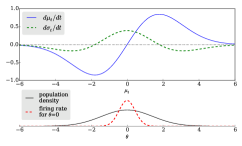
where gt=λ02πσtc2𝒩(μt;c,σt2+σtc2+σpop2)subscript𝑔𝑡superscript𝜆02𝜋superscriptsubscript𝜎tc2𝒩subscript𝜇𝑡𝑐superscriptsubscript𝜎𝑡2superscriptsubscript𝜎tc2superscriptsubscript𝜎pop2g_{t}=\lambda^{0}\sqrt{2\pi\sigma_{\mathrm{tc}}^{2}}\mathcal{N}\left(\mu_{t};c,\sigma_{t}^{2}+\sigma_{\mathrm{tc}}^{2}+\sigma_{\mathrm{pop}}^{2}\right). Figure 1 (left) shows how μt,σt2subscript𝜇𝑡superscriptsubscript𝜎𝑡2\mu_{t},\sigma_{t}^{2} change between spikes for a static 1-dimensional state (a=d=0𝑎𝑑0a=d=0). In this case, all terms in the filtering equations drop out except those involving gtsubscript𝑔𝑡g_{t}. The term involving gtsubscript𝑔𝑡g_{t} in dμt𝑑subscript𝜇𝑡d\mu_{t} pushes μtsubscript𝜇𝑡\mu_{t} away from c𝑐c in the absence of spikes. This effect weakens as |μtc|subscript𝜇𝑡𝑐\left|\mu_{t}-c\right| grows due to the factor gtsubscript𝑔𝑡g_{t}, consistent with the idea that far from c𝑐c, the lack of spikes is less surprising, hence less informative. The term involving gtsubscript𝑔𝑡g_{t} in dσt2𝑑superscriptsubscript𝜎𝑡2d\sigma_{t}^{2} increases the variance when μtsubscript𝜇𝑡\mu_{t} is near c𝑐c, otherwise decreases it.

Refer to caption
Refer to caption
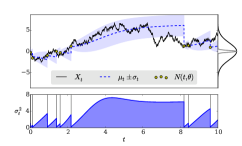
Figure 1: Left Changes to the posterior moments between spikes as a function of the current posterior mean estimate, for a static 1-d state. The parameters are a=d=0,H=1,σpop2=1,σtc2=0.2,c=0,λ0=10,σt=1formulae-sequence𝑎𝑑0formulae-sequence𝐻1formulae-sequencesuperscriptsubscript𝜎pop21formulae-sequencesuperscriptsubscript𝜎tc20.2formulae-sequence𝑐0formulae-sequencesuperscript𝜆010subscript𝜎𝑡1a=d=0,H=1,\sigma_{\mathrm{pop}}^{2}=1,\sigma_{\mathrm{tc}}^{2}=0.2,c=0,\lambda^{0}=10,\sigma_{t}=1. The bottom plot shows the density of preferred stimuli f(θ)𝑓𝜃f\left(\theta\right) and tuning curve for a neuron with preferred stimulus θ=0𝜃0\theta=0. Right An example of filtering a linear one-dimensional process. Each dot correspond to a spike with the vertical location indicating the preferred stimulus θ𝜃\theta. The curves to the right of the graph show the preferred stimulus density (black), and a tuning curve centered at θ=0𝜃0\theta=0 (gray). The tuning curve and preferred stimulus density are normalized to the same height for visualization. The bottom graph shows the posterior variance, with the vertical lines showing spike times. Parameters are: a=0.1,d=2,H=1,σpop2=2,σtc2=0.2,c=0,λ0=10,μ0=0,σ02=1formulae-sequence𝑎0.1formulae-sequence𝑑2formulae-sequence𝐻1formulae-sequencesuperscriptsubscript𝜎pop22formulae-sequencesuperscriptsubscript𝜎tc20.2formulae-sequence𝑐0formulae-sequencesuperscript𝜆010formulae-sequencesubscript𝜇00superscriptsubscript𝜎021a=-0.1,d=2,H=1,\sigma_{\mathrm{pop}}^{2}=2,\sigma_{\mathrm{tc}}^{2}=0.2,c=0,\lambda^{0}=10,\mu_{0}=0,\sigma_{0}^{2}=1. Note the decrease of the posterior variance following t=4𝑡4t=4 even though no spikes are observed.

3.3 Information from lack of spikes

An interesting aspect of the filtering equations (5)-(6) is that the dynamics of the posterior density between spikes differ from the prior dynamics. This is in contrast to previous models which assumed uniform coding: the (exact) filtering equations appearing in [23] and [24] have the same form as (5)-(6) except that they do not include the correction terms involving gtsubscript𝑔𝑡g_{t}, so that between spikes the dynamics are identical to the prior dynamics. This reflects the fact that lack of spikes in a time interval is an indication that the total firing rate is low; in the uniform coding case, this is not informative, since the total firing rate is independent of the state.

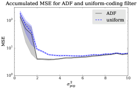
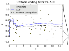
Figure 2 (left) illustrates the information gained from lack of spikes. A static scalar state is observed by a process with rate (2), and filtered twice: once with the correct value of σpopsubscript𝜎pop\sigma_{\mathrm{pop}}, and once with σpopsubscript𝜎pop\sigma_{\mathrm{pop}}\rightarrow\infty, as in the uniform coding filter of [24]. Between spikes, the ADF estimate moves away from the population center c=0𝑐0c=0, whereas the uniform coding estimate remains fixed. The size of this effect decreases with time, as the posterior variance estimate (not shown) decreases. The reduction in filtering errors gained from the additional terms in (5)-(6) is illustrated in Figure (2) (right). Despite the approximation involved, the full filter significantly outperforms the uniform coding filter. The difference disappears as σpopsubscript𝜎pop\sigma_{\mathrm{pop}} increases and the population becomes uniform.
Refer to caption
Refer to caption
Figure 2: Left Illustration of information gained between spikes. A static state Xt=0.5subscript𝑋𝑡0.5X_{t}=0.5, shown in a dotted line, is observed and filtered twice: with the correct value σpop2=0.5superscriptsubscript𝜎pop20.5\sigma_{\mathrm{pop}}^{2}=0.5 (“ADF”, solid blue line), and with σpop2=superscriptsubscript𝜎pop2\sigma_{\mathrm{pop}}^{2}=\infty (“Uniform coding filter”, dashed green line). The curves to the right of the graph show the preferred stimulus density (black), and a tuning curve centered at θ=0𝜃0\theta=0 (gray). Both filters are initialized with μ0=0,σ02=1formulae-sequencesubscript𝜇00superscriptsubscript𝜎021\mu_{0}=0,\sigma_{0}^{2}=1. Right Comparison of MSE for the ADF filter and the uniform coding filter. The vertical axis shows the integral of the square error integrated over the time interval [5,10]510\left[5,10\right], averaged over 1000 trials. Shaded areas indicate estimated errors, computed as the sample standard deviation divided by the square root of the number of trials. Parameters in both plots are a=d=0,c=0,σpop2=0.5,σtc2=0.1,H=1,λ0=10formulae-sequence𝑎𝑑0formulae-sequence𝑐0formulae-sequencesuperscriptsubscript𝜎pop20.5formulae-sequencesuperscriptsubscript𝜎tc20.1formulae-sequence𝐻1superscript𝜆010a=d=0,c=0,\sigma_{\mathrm{pop}}^{2}=0.5,\sigma_{\mathrm{tc}}^{2}=0.1,H=1,\lambda^{0}=10.

Special cases   To gain additional insight into the filtering equations, we consider their behavior in several limits. (i) As σpop2superscriptsubscript𝜎pop2\sigma_{\mathrm{pop}}^{2}\to\infty, spikes become rare as the density f(θ)𝑓𝜃f\left(\theta\right) approaches 0 for any θ𝜃\theta. The total expected rate of spikes gtsubscript𝑔𝑡g_{t} also approaches 0, and the terms corresponding to information from lack of spikes vanish. Other terms in the equations are unaffected. (ii) In the limit σtc2superscriptsubscript𝜎tc2\sigma_{\mathrm{tc}}^{2}\to\infty, each neuron fires as a Poisson process with a constant rate independent of the observed state. The total expected firing rate gtsubscript𝑔𝑡g_{t} saturates at its maximum, λ0superscript𝜆0\lambda^{0}. Therefore the preferred stimuli of spiking neurons provide no information, nor does the presence or absence of spikes. Accordingly, all terms other than those related to the prior dynamics vanish. (iii) The uniform coding case [23, 24] is obtained as a special case in the limit σpop2superscriptsubscript𝜎pop2\sigma_{\mathrm{pop}}^{2}\to\infty with λ0/σpopsuperscript𝜆0subscript𝜎pop\lambda^{0}/\sigma_{\mathrm{pop}} constant. In this limit the terms involving gtsubscript𝑔𝑡g_{t} drop out, recovering the (exact) filtering equations in [23].

4 Optimal neural encoding

We model the problem of optimal neural encoding as choosing the parameters c,Σpop,Σtc𝑐subscriptΣpopsubscriptΣtcc,\Sigma_{\mathrm{pop}},\Sigma_{\mathrm{tc}} of the population and tuning curves, so as to minimize the steady-state MSE. As noted above, when the estimate is exactly the posterior mean, this is equivalent to minimizing the steady-state expected posterior variance. The posterior variance has the advantage of being less noisy than the square error itself, since by definition it is the mean of the square error (of the posterior mean) under conditioning by 𝒩tsubscript𝒩𝑡\mathcal{N}_{t}. We explore the question of optimal neural encoding by measuring the steady-state variance through Monte Carlo simulations of the system dynamics and the filtering equations (5)-(6). Since the posterior mean and variance computed by ADF are approximate, we verified numerically that the variance closely matches the MSE in the steady state when averaged across many trials (see appendix), suggesting that asymptotically the error in estimating μtsubscript𝜇𝑡\mu_{t} and ΣtsubscriptΣ𝑡\Sigma_{t} is small.

4.1 Optimal population center

We now consider the question of the optimal value for the population center c𝑐c. Intuitively, if the prior distribution of the process X𝑋X is unimodal with mode x0subscript𝑥0x_{0}, the optimal population center is at Hx0𝐻subscript𝑥0Hx_{0}, to produce the most spikes. On the other hand, the terms involving gtsubscript𝑔𝑡g_{t} in the filtering equation (5)-(6) suggest that the lack of spikes is also informative. Moreover, as seen in Figure 1 (left), the posterior variance is reduced between spikes only when the current estimate is far enough from c𝑐c. These considerations suggest that there is a trade-off between maximizing the frequency of spikes and maximizing the information obtained from lack of spikes, yielding an optimal value for c𝑐c that differs from Hx0𝐻subscript𝑥0Hx_{0}.

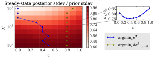
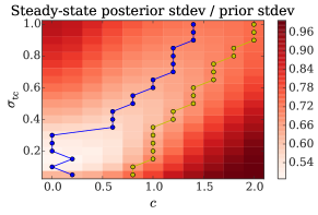
We simulated a simple one-dimensional process to determine the optimal value of c𝑐c which minimizes the approximate posterior variance ΣtsubscriptΣ𝑡\Sigma_{t}. Figure 3 (left) shows the posterior variance for varying values of the population center c𝑐c and base firing rate λ0superscript𝜆0\lambda^{0}. For each firing rate, we note the value of c𝑐c minimizing the posterior variance (the optimal population center), as well as the value of cm=argminc(dσt/dt|μt=0)subscript𝑐msubscriptargmin𝑐evaluated-at𝑑subscript𝜎𝑡𝑑𝑡subscript𝜇𝑡0c_{\mathrm{m}}=\mathrm{argmin}_{c}\left(d\sigma_{t}/dt|_{\mu_{t}=0}\right), which maximizes the reduction in the posterior variance when the current state estimate μtsubscript𝜇𝑡\mu_{t} is at the process equilibrium x0=0subscript𝑥00x_{0}=0. Consistent with the discussion above, the optimal value lies between 0 (where spikes are most abundant) and cmsubscript𝑐mc_{\mathrm{m}} (where lack of spikes is most informative). As could be expected, the optimal center is closer to 0 the higher the base firing rate. Similarly, wide tuning curves, which render the spikes less informative, lead to an optimal center farther from 0 (Figure 3, right).

A shift of the population center relative to the prior mode has been observed physiologically in encoding of inter-aural time differences for localization of sound sources [26]. In [18], this phenomenon was explained in a finite population model based on maximization of Fisher information. This is in contrast to the results of [21], which consider a heterogeneous population where the tuning curve width scales roughly inversely with neuron density. In this case, the population density maximizing the Fisher information is shown to be monotonic with the prior, i.e., more neurons should be assigned to more probable states. This apparent discrepancy may be due to the scaling of tuning curve widths in [21], which produces roughly constant total firing rate, i.e., uniform coding. This demonstrates that a non-constant total firing rate, which renders lack of spikes informative, may be necessary to explain the physiologically observed shift phenomenon.
Refer to caption
Refer to caption
Figure 3: Optimal population center location for filtering a linear one-dimensional process. Both graphs show the ratio of posterior standard deviation to the prior steady-state standard deviation of the process, along with the value of c𝑐c minimizing the posterior variance (blue line), and minimizing the reduction of posterior variance when μt=0subscript𝜇𝑡0\mu_{t}=0 (yellow line). The process is initialized from its steady-state distribution. The posterior variance is estimated by averaging over the time interval [5,10]510\left[5,10\right] and across 1000 trials for each data point. Parameters for both graphs: a=1,d=0.5,σpop2=0.1formulae-sequence𝑎1formulae-sequence𝑑0.5superscriptsubscript𝜎pop20.1a=-1,d=0.5,\sigma_{\mathrm{pop}}^{2}=0.1. In the graph on the left, σtc2=0.01superscriptsubscript𝜎tc20.01\sigma_{\mathrm{tc}}^{2}=0.01; on the right, λ0=50superscript𝜆050\lambda^{0}=50.

4.2 Optimization of population distribution

Next, we consider the optimization of the population distribution, namely, the simultaneous optimization of the population center c𝑐c and the population variance ΣpopsubscriptΣpop\Sigma_{\mathrm{pop}} in the case of a static scalar state. Previous work using a finite neuron population and a Fisher information-based criterion [18] has shown that the optimal distribution of preferred stimuli depends on the prior variance. When it is small relative to the tuning curve width, optimal encoding is achieved by placing all preferred stimuli at a fixed distance from the prior mean. On the other hand, when the prior variance is large relative to the tuning curve width, optimal encoding is uniform (see figure 2 in [18]).

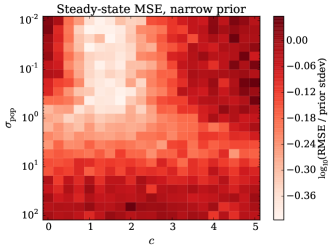
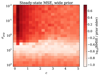
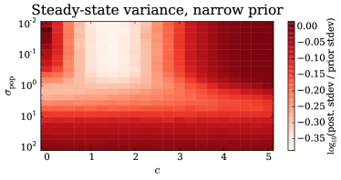
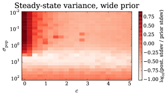
Similar results are obtained with our model, as shown in Figure 4. Here, a static scalar state drawn from 𝒩(0,σp2)𝒩0superscriptsubscript𝜎p2\mathcal{N}(0,\sigma_{\mathrm{p}}^{2}) is filtered by a population with tuning curve width σtc=1subscript𝜎tc1\sigma_{\mathrm{tc}}=1 and preferred stimulus density 𝒩(c,σpop2)𝒩𝑐superscriptsubscript𝜎pop2\mathcal{N}(c,\sigma_{\mathrm{pop}}^{2}). In Figure 4 (left), the prior distribution is narrow relative to the tuning curve width, leading to an optimal population with a narrow population distribution far from the origin. In Figure 4 (right), the prior is wide relative to the tuning curve width, leading to an optimal population with variance that roughly matches the prior variance. When both the tuning curves and the population density are narrow relative to the prior, so that spikes are rare (low values of σpopsubscript𝜎pop\sigma_{\mathrm{pop}} in Figure 4 (right)), the ADF approximation becomes poor, resulting in MSEs larger than the prior variance.
Refer to captionRefer to caption
Figure 4: Optimal population distribution depends on prior variance relative to tuning curve width. A static scalar state drawn from 𝒩(0,σp2)𝒩0superscriptsubscript𝜎p2\mathcal{N}(0,\sigma_{\mathrm{p}}^{2}) is filtered with tuning curve σtc=1subscript𝜎tc1\sigma_{\mathrm{tc}}=1 and preferred stimulus density 𝒩(c,σpop2)𝒩𝑐superscriptsubscript𝜎pop2\mathcal{N}(c,\sigma_{\mathrm{pop}}^{2}). Both graphs show the posterior standard deviation relative to the prior standard deviation σpsubscript𝜎p\sigma_{\mathrm{p}}. In the left graph, the prior distribution is narrow, σp2=0.1superscriptsubscript𝜎p20.1\sigma_{\mathrm{p}}^{2}=0.1, whereas on the right, it is wide, σp2=10superscriptsubscript𝜎p210\sigma_{\mathrm{p}}^{2}=10. In both cases the filter is initialized with the correct prior, and the square error is averaged over the time interval [5,10]510\left[5,10\right] and across 100 trials for each data point.

5 Conclusions

We have introduced an analytically tractable Bayesian approximation to point process filtering, allowing us to gain insight into the generally intractable infinite-dimensional filtering problem. The approach enables the derivation of near-optimal encoding schemes going beyond previously studied uniform coding assumptions. The framework is presented in continuous time, circumventing temporal discretization errors and numerical imprecisions in sampling-based methods, applies to fully dynamic setups, and directly estimates the MSE rather than lower bounds to it. It successfully explains observed experimental results, and opens the door to many future predictions. Future work will include a development of previously successful mean field approaches [13] within our more general framework, leading to further analytic insight. Moreover, the proposed strategy may lead to practically useful decoding of spike trains.

Appendix A Appendix

A.1 Derivation of the ADF filtering equations for linear dynamics

A.1.1 Setting and notation

In the main text, we have presented our model in an open-loop setting, where the process X𝑋X is passively observed. Here we consider a more general setting, incorporating a control process Utsubscript𝑈𝑡U_{t}, so the dynamics are

dXt=(A(Xt)+B(Ut))dt+D(Xt)dWt,𝑑subscript𝑋𝑡𝐴subscript𝑋𝑡𝐵subscript𝑈𝑡𝑑𝑡𝐷subscript𝑋𝑡𝑑subscript𝑊𝑡dX_{t}=\left(A\left(X_{t}\right)+B\left(U_{t}\right)\right)dt+D\left(X_{t}\right)dW_{t}, (9)

where, in general, Utsubscript𝑈𝑡U_{t} is a function of 𝒩tsubscript𝒩𝑡\mathcal{N}_{t}.

For the purposes of the derivation, it is convenient to work with precision matrices rather than variance matrices. We write F=Σpop1,R=Σtc1formulae-sequence𝐹superscriptsubscriptΣpop1𝑅superscriptsubscriptΣtc1F=\Sigma_{\mathrm{pop}}^{-1},R=\Sigma_{\mathrm{tc}}^{-1} and Qt=Σt1subscript𝑄𝑡superscriptsubscriptΣ𝑡1Q_{t}=\Sigma_{t}^{-1}. Thus the density of the process N𝑁N at (t,θ)𝑡𝜃\left(t,\theta\right) given X[0,t]subscript𝑋0𝑡X_{\left[0,t\right]} is

λt(θ,Xt)subscript𝜆𝑡𝜃subscript𝑋𝑡\displaystyle\lambda_{t}\left(\theta,X_{t}\right) =λ0|F|(2π)mexp(12θcF212HXtθR2),absentsuperscript𝜆0𝐹superscript2𝜋𝑚12superscriptsubscriptnorm𝜃𝑐𝐹212superscriptsubscriptnorm𝐻subscript𝑋𝑡𝜃𝑅2\displaystyle=\lambda^{0}\sqrt{\frac{\left|F\right|}{\left(2\pi\right)^{m}}}\exp\left(-\frac{1}{2}\left\|\theta-c\right\|_{F}^{2}-\frac{1}{2}\left\|HX_{t}-\theta\right\|_{R}^{2}\right), (10)
=λ0|F|(2π)mexp(12HXtcM212θ(F+R)1(Fc+RHXt)F+R2),absentsuperscript𝜆0𝐹superscript2𝜋𝑚12superscriptsubscriptnorm𝐻subscript𝑋𝑡𝑐𝑀212superscriptsubscriptnorm𝜃superscript𝐹𝑅1𝐹𝑐𝑅𝐻subscript𝑋𝑡𝐹𝑅2\displaystyle=\lambda^{0}\sqrt{\frac{\left|F\right|}{\left(2\pi\right)^{m}}}\exp\left(-\frac{1}{2}\left\|HX_{t}-c\right\|_{M}^{2}-\frac{1}{2}\left\|\theta-\left(F+R\right)^{-1}\left(Fc+RHX_{t}\right)\right\|_{F+R}^{2}\right), (11)

where M(F1+R1)1𝑀superscriptsuperscript𝐹1superscript𝑅11M\triangleq\left(F^{-1}+R^{-1}\right)^{-1}.

We denote by P(,t)𝑃𝑡P\left(\cdot,t\right) the posterior density of Xtsubscript𝑋𝑡X_{t} given 𝒩tsubscript𝒩𝑡\mathcal{N}_{t}, and by EPt[]superscriptsubscriptE𝑃𝑡delimited-[]\mathrm{E}_{P}^{t}\left[\cdot\right] the posterior expectation based on observations up to time t𝑡t. We will simply write EP[]subscriptE𝑃delimited-[]\mathrm{E}_{P}\left[\cdot\right] when the time t𝑡t is obvious from context.

A.1.2 Filtering equations between spikes

Exact filtering equations for the first two moments

As seen in [23], the PDE for the posterior density,

dtP(x,t)=tP(x,t)dt+P(x,t)nλt(θ,x)λ^t(θ)λ^t(θ)(N(dt×dθ)λ^t(θ)dθdt),subscript𝑑𝑡𝑃𝑥𝑡superscriptsubscript𝑡𝑃𝑥𝑡𝑑𝑡𝑃𝑥𝑡subscriptsuperscript𝑛subscript𝜆𝑡𝜃𝑥subscript^𝜆𝑡𝜃subscript^𝜆𝑡𝜃𝑁𝑑𝑡𝑑𝜃subscript^𝜆𝑡𝜃𝑑𝜃𝑑𝑡d_{t}P\left(x,t\right)=\mathcal{L}_{t}^{*}P\left(x,t\right)dt+P\left(x,t\right)\int_{\mathbb{R}^{n}}\frac{\lambda_{t}\left(\theta,x\right)-\hat{\lambda}_{t}\left(\theta\right)}{\hat{\lambda}_{t}\left(\theta\right)}\left(N\left(dt\times d\theta\right)-\hat{\lambda}_{t}\left(\theta\right)d\theta\,dt\right), (12)

still holds in the closed-loop case. Here tsubscript𝑡\mathcal{L}_{t} (appearing in place of \mathcal{L} in (3)) is the posterior infinitesimal generator, defined with an additional conditioning on 𝒩tsubscript𝒩𝑡\mathcal{N}_{t},

tf(x)=limΔt0+E[f(Xt+Δt)|Xt=x,𝒩t]f(x)Δt,subscript𝑡𝑓𝑥subscriptΔ𝑡superscript0Edelimited-[]conditional𝑓subscript𝑋𝑡Δ𝑡subscript𝑋𝑡𝑥subscript𝒩𝑡𝑓𝑥Δ𝑡\mathcal{L}_{t}f\left(x\right)=\lim_{\Delta t\to 0^{+}}\frac{\mathrm{E}\left[f\left(X_{t+\Delta t}\right)|X_{t}=x,\mathcal{N}_{t}\right]-f\left(x\right)}{\Delta t},

and tsuperscriptsubscript𝑡\mathcal{L}_{t}^{*} is its adjoint. Note that in this closed-loop setting, the infinitesimal generator is itself a random operator, due to its dependence on past observations through the control law, and that Ntsubscript𝑁𝑡N_{t} is no longer a doubly-stochastic Poisson process.

Between spikes, (12) simplifies to

tP(x,t)=tP(x,t)P(x,t)n(λt(θ,x)λ^t(θ))𝑑θ,𝑡𝑃𝑥𝑡superscriptsubscript𝑡𝑃𝑥𝑡𝑃𝑥𝑡subscriptsuperscript𝑛subscript𝜆𝑡𝜃𝑥subscript^𝜆𝑡𝜃differential-d𝜃\frac{\partial}{\partial t}P\left(x,t\right)=\mathcal{L}_{t}^{*}P\left(x,t\right)-P\left(x,t\right)\int_{\mathbb{R}^{n}}\left(\lambda_{t}\left(\theta,x\right)-\hat{\lambda}_{t}\left(\theta\right)\right)d\theta,

so for a sufficiently well-behaved function f𝑓f,

EP[f(Xt)]tsubscriptE𝑃delimited-[]𝑓subscript𝑋𝑡𝑡\displaystyle\frac{\partial\mathrm{E}_{P}\left[f\left(X_{t}\right)\right]}{\partial t} =\displaystyle= f(x)(tP(x,t)+P(x,t)(λ^t(θ)λt(θ,x))𝑑θ)𝑑x𝑓𝑥superscriptsubscript𝑡𝑃𝑥𝑡𝑃𝑥𝑡subscript^𝜆𝑡𝜃subscript𝜆𝑡𝜃𝑥differential-d𝜃differential-d𝑥\displaystyle\int f\left(x\right)\left(\mathcal{L}_{t}^{*}P\left(x,t\right)+P\left(x,t\right)\int\left(\hat{\lambda}_{t}\left(\theta\right)-\lambda_{t}\left(\theta,x\right)\right)d\theta\right)dx
=\displaystyle= P(x,t)(tf(x)+f(x)(λ^t(θ)λt(θ,x))𝑑θ)𝑑x𝑃𝑥𝑡subscript𝑡𝑓𝑥𝑓𝑥subscript^𝜆𝑡𝜃subscript𝜆𝑡𝜃𝑥differential-d𝜃differential-d𝑥\displaystyle\int P\left(x,t\right)\left(\mathcal{L}_{t}f\left(x\right)+f\left(x\right)\int\left(\hat{\lambda}_{t}\left(\theta\right)-\lambda_{t}\left(\theta,x\right)\right)d\theta\right)dx
=\displaystyle= EP[tf(Xt)+f(Xt)(λ^t(θ)λt(θ,Xt))𝑑θ].subscriptE𝑃delimited-[]subscript𝑡𝑓subscript𝑋𝑡𝑓subscript𝑋𝑡subscript^𝜆𝑡𝜃subscript𝜆𝑡𝜃subscript𝑋𝑡differential-d𝜃\displaystyle\mathrm{E}_{P}\left[\mathcal{L}_{t}f\left(X_{t}\right)+f\left(X_{t}\right)\int\left(\hat{\lambda}_{t}\left(\theta\right)-\lambda_{t}\left(\theta,X_{t}\right)\right)d\theta\right].

Assuming the state evolves as in (9), the (closed loop) infinitesimal generator is

tf(x)=(A(x)+B(Ut))Tf(x)+12Tr[2f(x)D(x)D(x)T],subscript𝑡𝑓𝑥superscript𝐴𝑥𝐵subscript𝑈𝑡𝑇𝑓𝑥12Trdelimited-[]superscript2𝑓𝑥𝐷𝑥𝐷superscript𝑥𝑇\mathcal{L}_{t}f\left(x\right)=\left(A\left(x\right)+B\left(U_{t}\right)\right)^{T}\nabla f\left(x\right)+\frac{1}{2}\mathrm{Tr}\left[\nabla^{2}f\left(x\right)D\left(x\right)D\left(x\right)^{T}\right],

so, letting μt=EPXt,X~t=Xtμt,Σt=EP[X~tX~tT]formulae-sequencesubscript𝜇𝑡subscriptE𝑃subscript𝑋𝑡formulae-sequencesubscript~𝑋𝑡subscript𝑋𝑡subscript𝜇𝑡subscriptΣ𝑡subscriptE𝑃delimited-[]subscript~𝑋𝑡superscriptsubscript~𝑋𝑡𝑇\mu_{t}=\mathrm{E}_{P}X_{t},\tilde{X}_{t}=X_{t}-\mu_{t},\Sigma_{t}=\mathrm{E}_{P}\left[\tilde{X}_{t}\tilde{X}_{t}^{T}\right],

dμtdt𝑑subscript𝜇𝑡𝑑𝑡\displaystyle\frac{d\mu_{t}}{dt} =\displaystyle= EP[A(Xt)]+B(Ut)+EP[Xt(λ^t(θ)λt(θ,Xt))𝑑θ],subscriptE𝑃delimited-[]𝐴subscript𝑋𝑡𝐵subscript𝑈𝑡subscriptE𝑃delimited-[]subscript𝑋𝑡subscript^𝜆𝑡𝜃subscript𝜆𝑡𝜃subscript𝑋𝑡differential-d𝜃\displaystyle\mathrm{E}_{P}\left[A\left(X_{t}\right)\right]+B\left(U_{t}\right)+\mathrm{E}_{P}\left[X_{t}\int\left(\hat{\lambda}_{t}\left(\theta\right)-\lambda_{t}\left(\theta,X_{t}\right)\right)d\theta\right],
dΣtdt𝑑subscriptΣ𝑡𝑑𝑡\displaystyle\frac{d\Sigma_{t}}{dt} =\displaystyle= EP[A(Xt)X~tT]+EP[X~tA(Xt)T]+EP[D(Xt)D(Xt)T]subscriptE𝑃delimited-[]𝐴subscript𝑋𝑡superscriptsubscript~𝑋𝑡𝑇subscriptE𝑃delimited-[]subscript~𝑋𝑡𝐴superscriptsubscript𝑋𝑡𝑇subscriptE𝑃delimited-[]𝐷subscript𝑋𝑡𝐷superscriptsubscript𝑋𝑡𝑇\displaystyle\mathrm{E}_{P}\left[A\left(X_{t}\right)\tilde{X}_{t}^{T}\right]+\mathrm{E}_{P}\left[\tilde{X}_{t}A\left(X_{t}\right)^{T}\right]+\mathrm{E}_{P}\left[D\left(X_{t}\right)D\left(X_{t}\right)^{T}\right] (13)
+EP[X~tX~tT(λ^t(θ)λt(θ,Xt))𝑑θ],subscriptE𝑃delimited-[]subscript~𝑋𝑡superscriptsubscript~𝑋𝑡𝑇subscript^𝜆𝑡𝜃subscript𝜆𝑡𝜃subscript𝑋𝑡differential-d𝜃\displaystyle+\mathrm{E}_{P}\left[\tilde{X}_{t}\tilde{X}_{t}^{T}\int\left(\hat{\lambda}_{t}\left(\theta\right)-\lambda_{t}\left(\theta,X_{t}\right)\right)d\theta\right],

which is the same as (4), with an additional term B(Ut)𝐵subscript𝑈𝑡B\left(U_{t}\right).

ADF approximation

The computations that follow frequently require multiplying Gaussian functions, sometimes with a possibly degenerate precision matrix. To this end, we use the following slightly generalized form of a well-known result about the sum of quadratic forms.

Claim.

Let x,a,bn𝑥𝑎𝑏superscript𝑛x,a,b\in\mathbb{R}^{n} and A,Bn×n𝐴𝐵superscript𝑛𝑛A,B\in\mathbb{R}^{n\times n} be symmetric matrices such that A+B𝐴𝐵A+B is non-singular. Then

xaA2+xbB2=abA(A+B)1B2+x(A+B)1(Aa+Bb)A+B2.superscriptsubscriptnorm𝑥𝑎𝐴2superscriptsubscriptnorm𝑥𝑏𝐵2superscriptsubscriptnorm𝑎𝑏𝐴superscript𝐴𝐵1𝐵2superscriptsubscriptnorm𝑥superscript𝐴𝐵1𝐴𝑎𝐵𝑏𝐴𝐵2\left\|x-a\right\|_{A}^{2}+\left\|x-b\right\|_{B}^{2}=\left\|a-b\right\|_{A\left(A+B\right)^{-1}B}^{2}+\left\|x-\left(A+B\right)^{-1}\left(Aa+Bb\right)\right\|_{A+B}^{2}.
Proof.

This is proved by a straightforward completion of squares. If A,B𝐴𝐵A,B are invertible,

xaA2+xbB2superscriptsubscriptnorm𝑥𝑎𝐴2superscriptsubscriptnorm𝑥𝑏𝐵2\displaystyle\left\|x-a\right\|_{A}^{2}+\left\|x-b\right\|_{B}^{2} =\displaystyle= xA2xTAaaTAx+aA2+xB2xTBbbTBx+bB2superscriptsubscriptnorm𝑥𝐴2superscript𝑥𝑇𝐴𝑎superscript𝑎𝑇𝐴𝑥superscriptsubscriptnorm𝑎𝐴2superscriptsubscriptnorm𝑥𝐵2superscript𝑥𝑇𝐵𝑏superscript𝑏𝑇𝐵𝑥superscriptsubscriptnorm𝑏𝐵2\displaystyle\left\|x\right\|_{A}^{2}-x^{T}Aa-a^{T}Ax+\left\|a\right\|_{A}^{2}+\left\|x\right\|_{B}^{2}-x^{T}Bb-b^{T}Bx+\left\|b\right\|_{B}^{2}
=\displaystyle= xA+B2xT(Aa+Bb)(Aa+Bb)Tx+aA2+bB2superscriptsubscriptnorm𝑥𝐴𝐵2superscript𝑥𝑇𝐴𝑎𝐵𝑏superscript𝐴𝑎𝐵𝑏𝑇𝑥superscriptsubscriptnorm𝑎𝐴2superscriptsubscriptnorm𝑏𝐵2\displaystyle\left\|x\right\|_{A+B}^{2}-x^{T}\left(Aa+Bb\right)-\left(Aa+Bb\right)^{T}x+\left\|a\right\|_{A}^{2}+\left\|b\right\|_{B}^{2}
=\displaystyle= x(A+B)1(Aa+Bb)A+B2(A+B)1(Aa+Bb)A+B2+aA2+bB2superscriptsubscriptnorm𝑥superscript𝐴𝐵1𝐴𝑎𝐵𝑏𝐴𝐵2superscriptsubscriptnormsuperscript𝐴𝐵1𝐴𝑎𝐵𝑏𝐴𝐵2superscriptsubscriptnorm𝑎𝐴2superscriptsubscriptnorm𝑏𝐵2\displaystyle\left\|x-\left(A+B\right)^{-1}\left(Aa+Bb\right)\right\|_{A+B}^{2}-\left\|\left(A+B\right)^{-1}\left(Aa+Bb\right)\right\|_{A+B}^{2}+\left\|a\right\|_{A}^{2}+\left\|b\right\|_{B}^{2}
=\displaystyle= x(A+B)1(Aa+Bb)A+B2+aA2+bB2Aa+Bb(A+B)12superscriptsubscriptnorm𝑥superscript𝐴𝐵1𝐴𝑎𝐵𝑏𝐴𝐵2subscriptsuperscriptsubscriptnorm𝑎𝐴2superscriptsubscriptnorm𝑏𝐵2superscriptsubscriptnorm𝐴𝑎𝐵𝑏superscript𝐴𝐵12\displaystyle\left\|x-\left(A+B\right)^{-1}\left(Aa+Bb\right)\right\|_{A+B}^{2}+\underbrace{\left\|a\right\|_{A}^{2}+\left\|b\right\|_{B}^{2}-\left\|Aa+Bb\right\|_{\left(A+B\right)^{-1}}^{2}}_{*}
\displaystyle* =\displaystyle= aA2+bB2Aa(A+B)12aTA(A+B)1BbbTB(A+B)1AaBb(A+B)12superscriptsubscriptnorm𝑎𝐴2superscriptsubscriptnorm𝑏𝐵2superscriptsubscriptnorm𝐴𝑎superscript𝐴𝐵12superscript𝑎𝑇𝐴superscript𝐴𝐵1𝐵𝑏superscript𝑏𝑇𝐵superscript𝐴𝐵1𝐴𝑎superscriptsubscriptnorm𝐵𝑏superscript𝐴𝐵12\displaystyle\left\|a\right\|_{A}^{2}+\left\|b\right\|_{B}^{2}-\left\|Aa\right\|_{\left(A+B\right)^{-1}}^{2}-a^{T}A\left(A+B\right)^{-1}Bb-b^{T}B\left(A+B\right)^{-1}Aa-\left\|Bb\right\|_{\left(A+B\right)^{-1}}^{2}
=\displaystyle= aTA(a(A+B)1Aa(A+B)1Bb)+bTB(b(A+B)1Bb(A+B)1Aa)superscript𝑎𝑇𝐴𝑎superscript𝐴𝐵1𝐴𝑎superscript𝐴𝐵1𝐵𝑏superscript𝑏𝑇𝐵𝑏superscript𝐴𝐵1𝐵𝑏superscript𝐴𝐵1𝐴𝑎\displaystyle a^{T}A\left(a-\left(A+B\right)^{-1}Aa-\left(A+B\right)^{-1}Bb\right)+b^{T}B\left(b-\left(A+B\right)^{-1}Bb-\left(A+B\right)^{-1}Aa\right)
=\displaystyle= aTA(A+B)1B(ab)+bTB(A+B)1A(ba)superscript𝑎𝑇𝐴superscript𝐴𝐵1𝐵𝑎𝑏superscript𝑏𝑇𝐵superscript𝐴𝐵1𝐴𝑏𝑎\displaystyle a^{T}A\left(A+B\right)^{-1}B\left(a-b\right)+b^{T}B\left(A+B\right)^{-1}A\left(b-a\right)
=\displaystyle= aT(B1+A1)1(ab)+bT(A1+B1)1(ba)superscript𝑎𝑇superscriptsuperscript𝐵1superscript𝐴11𝑎𝑏superscript𝑏𝑇superscriptsuperscript𝐴1superscript𝐵11𝑏𝑎\displaystyle a^{T}\left(B^{-1}+A^{-1}\right)^{-1}\left(a-b\right)+b^{T}\left(A^{-1}+B^{-1}\right)^{-1}\left(b-a\right)
=\displaystyle= ab(A1+B1)12superscriptsubscriptnorm𝑎𝑏superscriptsuperscript𝐴1superscript𝐵112\displaystyle\left\|a-b\right\|_{\left(A^{-1}+B^{-1}\right)^{-1}}^{2}
=\displaystyle= abA(A+B)1B2superscriptsubscriptnorm𝑎𝑏𝐴superscript𝐴𝐵1𝐵2\displaystyle\left\|a-b\right\|_{A\left(A+B\right)^{-1}B}^{2}

By continuity, the claim also holds when A,B𝐴𝐵A,B are not both invertible, provided (A+B)𝐴𝐵\left(A+B\right) is invertible. ∎

Computing the expectations in (13) involves computation of integrals containing P(x,t)λt(θ,x)𝑃𝑥𝑡subscript𝜆𝑡𝜃𝑥P\left(x,t\right)\lambda_{t}\left(\theta,x\right). Taking the ADF approximation P(x,t)𝒩(x;μt,Σt)𝑃𝑥𝑡𝒩𝑥subscript𝜇𝑡subscriptΣ𝑡P\left(x,t\right)\approx\mathcal{N}\left(x;\mu_{t},\Sigma_{t}\right), and using the claim above, we have

P(x,t)λt(θ,x)𝑃𝑥𝑡subscript𝜆𝑡𝜃𝑥\displaystyle P\left(x,t\right)\lambda_{t}\left(\theta,x\right) \displaystyle\approx λ0|F|(2π)m𝒩(x;μt,Σt)exp(12(HxcM2+θ(F+R)1(Fc+RHx)F+R2))superscript𝜆0𝐹superscript2𝜋𝑚𝒩𝑥subscript𝜇𝑡subscriptΣ𝑡12superscriptsubscriptnorm𝐻𝑥𝑐𝑀2superscriptsubscriptnorm𝜃superscript𝐹𝑅1𝐹𝑐𝑅𝐻𝑥𝐹𝑅2\displaystyle\lambda^{0}\sqrt{\frac{\left|F\right|}{\left(2\pi\right)^{m}}}\mathcal{N}\left(x;\mu_{t},\Sigma_{t}\right)\exp\left(-\frac{1}{2}\left(\left\|Hx-c\right\|_{M}^{2}+\left\|\theta-\left(F+R\right)^{-1}\left(Fc+RHx\right)\right\|_{F+R}^{2}\right)\right)
=\displaystyle= λ0|F|(2π)m+n|Σt|exp(12xμtQt2)superscript𝜆0𝐹superscript2𝜋𝑚𝑛subscriptΣ𝑡12superscriptsubscriptnorm𝑥subscript𝜇𝑡subscript𝑄𝑡2\displaystyle\lambda^{0}\sqrt{\frac{\left|F\right|}{\left(2\pi\right)^{m+n}\left|\Sigma_{t}\right|}}\exp\left(-\frac{1}{2}\left\|x-\mu_{t}\right\|_{Q_{t}}^{2}\right)
×exp(12(xc¯HTMH2+θ(F+R)1(Fc+RHx)F+R2))absent12superscriptsubscriptnorm𝑥¯𝑐superscript𝐻𝑇𝑀𝐻2superscriptsubscriptnorm𝜃superscript𝐹𝑅1𝐹𝑐𝑅𝐻𝑥𝐹𝑅2\displaystyle\times\exp\left(-\frac{1}{2}\left(\left\|x-\bar{c}\right\|_{H^{T}MH}^{2}+\left\|\theta-\left(F+R\right)^{-1}\left(Fc+RHx\right)\right\|_{F+R}^{2}\right)\right)
=\displaystyle= λ0|F|(2π)m+n|Σt|exp(12(μtc¯QtM2+xμtMQt+HTMH2))superscript𝜆0𝐹superscript2𝜋𝑚𝑛subscriptΣ𝑡12superscriptsubscriptnormsubscript𝜇𝑡¯𝑐superscriptsubscript𝑄𝑡𝑀2superscriptsubscriptnorm𝑥superscriptsubscript𝜇𝑡𝑀subscript𝑄𝑡superscript𝐻𝑇𝑀𝐻2\displaystyle\lambda^{0}\sqrt{\frac{\left|F\right|}{\left(2\pi\right)^{m+n}\left|\Sigma_{t}\right|}}\exp\left(-\frac{1}{2}\left(\left\|\mu_{t}-\bar{c}\right\|_{Q_{t}^{M}}^{2}+\left\|x-\mu_{t}^{M}\right\|_{Q_{t}+H^{T}MH}^{2}\right)\right)
×exp(12θ(F+R)1(Fc+RHx)F+R2)absent12superscriptsubscriptnorm𝜃superscript𝐹𝑅1𝐹𝑐𝑅𝐻𝑥𝐹𝑅2\displaystyle\times\exp\left(-\frac{1}{2}\left\|\theta-\left(F+R\right)^{-1}\left(Fc+RHx\right)\right\|_{F+R}^{2}\right)

where Hr1superscriptsubscript𝐻𝑟1H_{r}^{-1} is any right inverse of H𝐻H, and

c¯¯𝑐\displaystyle\bar{c} \displaystyle\triangleq Hr1csuperscriptsubscript𝐻𝑟1𝑐\displaystyle H_{r}^{-1}c
M𝑀\displaystyle M \displaystyle\triangleq F(F+R)1R=(F1+R1)1𝐹superscript𝐹𝑅1𝑅superscriptsuperscript𝐹1superscript𝑅11\displaystyle F\left(F+R\right)^{-1}R=\left(F^{-1}+R^{-1}\right)^{-1}
μtMsuperscriptsubscript𝜇𝑡𝑀\displaystyle\mu_{t}^{M} \displaystyle\triangleq (Qt+HTMH)1(Qtμt+HTMHc¯)superscriptsubscript𝑄𝑡superscript𝐻𝑇𝑀𝐻1subscript𝑄𝑡subscript𝜇𝑡superscript𝐻𝑇𝑀𝐻¯𝑐\displaystyle\left(Q_{t}+H^{T}MH\right)^{-1}\left(Q_{t}\mu_{t}+H^{T}MH\bar{c}\right)
QtMsuperscriptsubscript𝑄𝑡𝑀\displaystyle Q_{t}^{M} \displaystyle\triangleq Qt(Qt+HTMH)1HTMH=(I+HTMHΣt)1HTMH.subscript𝑄𝑡superscriptsubscript𝑄𝑡superscript𝐻𝑇𝑀𝐻1superscript𝐻𝑇𝑀𝐻superscript𝐼superscript𝐻𝑇𝑀𝐻subscriptΣ𝑡1superscript𝐻𝑇𝑀𝐻\displaystyle Q_{t}\left(Q_{t}+H^{T}MH\right)^{-1}H^{T}MH=\left(I+H^{T}MH\Sigma_{t}\right)^{-1}H^{T}MH.

An alternate form for QtMsuperscriptsubscript𝑄𝑡𝑀Q_{t}^{M} may be derived from the Woodbury identity as follows,

QtMsuperscriptsubscript𝑄𝑡𝑀\displaystyle Q_{t}^{M} =\displaystyle= (I+HTMHΣt)1HTMHsuperscript𝐼superscript𝐻𝑇𝑀𝐻subscriptΣ𝑡1superscript𝐻𝑇𝑀𝐻\displaystyle\left(I+H^{T}MH\Sigma_{t}\right)^{-1}H^{T}MH (14)
=\displaystyle= (IHT(M1+HΣtHT)1HΣt)HTMH𝐼superscript𝐻𝑇superscriptsuperscript𝑀1𝐻subscriptΣ𝑡superscript𝐻𝑇1𝐻subscriptΣ𝑡superscript𝐻𝑇𝑀𝐻\displaystyle\left(I-H^{T}\left(M^{-1}+H\Sigma_{t}H^{T}\right)^{-1}H\Sigma_{t}\right)H^{T}MH
=\displaystyle= HT(I(M1+HΣtHT)1HΣtHT)MHsuperscript𝐻𝑇𝐼superscriptsuperscript𝑀1𝐻subscriptΣ𝑡superscript𝐻𝑇1𝐻subscriptΣ𝑡superscript𝐻𝑇𝑀𝐻\displaystyle H^{T}\left(I-\left(M^{-1}+H\Sigma_{t}H^{T}\right)^{-1}H\Sigma_{t}H^{T}\right)MH
=\displaystyle= HT((M1+HΣtHT)1M1)MHsuperscript𝐻𝑇superscriptsuperscript𝑀1𝐻subscriptΣ𝑡superscript𝐻𝑇1superscript𝑀1𝑀𝐻\displaystyle H^{T}\left(\left(M^{-1}+H\Sigma_{t}H^{T}\right)^{-1}M^{-1}\right)MH
=\displaystyle= HTStMH,superscript𝐻𝑇superscriptsubscript𝑆𝑡𝑀𝐻\displaystyle H^{T}S_{t}^{M}H,

where

StM(M1+HΣtHT)1,superscriptsubscript𝑆𝑡𝑀superscriptsuperscript𝑀1𝐻subscriptΣ𝑡superscript𝐻𝑇1S_{t}^{M}\triangleq\left(M^{-1}+H\Sigma_{t}H^{T}\right)^{-1},

so we can write

P(x,t)λt(θ,x)𝑃𝑥𝑡subscript𝜆𝑡𝜃𝑥\displaystyle P\left(x,t\right)\lambda_{t}\left(\theta,x\right) \displaystyle\approx λ0|F|(2π)m+n|Σt|exp(12(HμtcStM2+xμtMQt+HTMH2))superscript𝜆0𝐹superscript2𝜋𝑚𝑛subscriptΣ𝑡12superscriptsubscriptnorm𝐻subscript𝜇𝑡𝑐superscriptsubscript𝑆𝑡𝑀2superscriptsubscriptnorm𝑥superscriptsubscript𝜇𝑡𝑀subscript𝑄𝑡superscript𝐻𝑇𝑀𝐻2\displaystyle\lambda^{0}\sqrt{\frac{\left|F\right|}{\left(2\pi\right)^{m+n}\left|\Sigma_{t}\right|}}\exp\left(-\frac{1}{2}\left(\left\|H\mu_{t}-c\right\|_{S_{t}^{M}}^{2}+\left\|x-\mu_{t}^{M}\right\|_{Q_{t}+H^{T}MH}^{2}\right)\right)
×exp(12θ(F+R)1(Fc+RHx)F+R2).absent12superscriptsubscriptnorm𝜃superscript𝐹𝑅1𝐹𝑐𝑅𝐻𝑥𝐹𝑅2\displaystyle\times\exp\left(-\frac{1}{2}\left\|\theta-\left(F+R\right)^{-1}\left(Fc+RHx\right)\right\|_{F+R}^{2}\right).

Now we define

gtλ^t(θ)𝑑θ=EP[λt(θ,Xt)]𝑑θ,subscript𝑔𝑡subscript^𝜆𝑡𝜃differential-d𝜃subscriptE𝑃delimited-[]subscript𝜆𝑡𝜃subscript𝑋𝑡differential-d𝜃g_{t}\triangleq\int\hat{\lambda}_{t}\left(\theta\right)d\theta=\int\mathrm{E}_{P}\left[\lambda_{t}\left(\theta,X_{t}\right)\right]d\theta,

and compute its value as follows:

gtsubscript𝑔𝑡\displaystyle g_{t} =\displaystyle= λ^t(θ)𝑑θsubscript^𝜆𝑡𝜃differential-d𝜃\displaystyle\int\hat{\lambda}_{t}\left(\theta\right)d\theta
=\displaystyle= P(x,t)λt(θ,x)𝑑x𝑑θ𝑃𝑥𝑡subscript𝜆𝑡𝜃𝑥differential-d𝑥differential-d𝜃\displaystyle\int\int P\left(x,t\right)\lambda_{t}\left(\theta,x\right)dxd\theta
\displaystyle\approx λ0detF(2π)m+ndetΣtexp(12HμtcStM2)𝑑xexp(12xμtMQt+HTMH2)superscript𝜆0𝐹superscript2𝜋𝑚𝑛subscriptΣ𝑡12superscriptsubscriptnorm𝐻subscript𝜇𝑡𝑐superscriptsubscript𝑆𝑡𝑀2differential-d𝑥12superscriptsubscriptnorm𝑥superscriptsubscript𝜇𝑡𝑀subscript𝑄𝑡superscript𝐻𝑇𝑀𝐻2\displaystyle\lambda^{0}\sqrt{\frac{\det F}{\left(2\pi\right)^{m+n}\det\Sigma_{t}}}\exp\left(-\frac{1}{2}\left\|H\mu_{t}-c\right\|_{S_{t}^{M}}^{2}\right)\int dx\exp\left(-\frac{1}{2}\left\|x-\mu_{t}^{M}\right\|_{Q_{t}+H^{T}MH}^{2}\right)
×dθexp(12θ(F+R)1(Fc+RHx)F+R2)\displaystyle\times\int d\theta\exp\left(-\frac{1}{2}\left\|\theta-\left(F+R\right)^{-1}\left(Fc+RHx\right)\right\|_{F+R}^{2}\right)
=\displaystyle= λ0detF(2π)ndetΣtdet(F+R)exp(12HμtcStM2)superscript𝜆0𝐹superscript2𝜋𝑛subscriptΣ𝑡𝐹𝑅12superscriptsubscriptnorm𝐻subscript𝜇𝑡𝑐superscriptsubscript𝑆𝑡𝑀2\displaystyle\lambda^{0}\sqrt{\frac{\det F}{\left(2\pi\right)^{n}\det\Sigma_{t}\det\left(F+R\right)}}\exp\left(-\frac{1}{2}\left\|H\mu_{t}-c\right\|_{S_{t}^{M}}^{2}\right)
𝑑xexp(12xμtMQt+HTMH2)differential-d𝑥12superscriptsubscriptnorm𝑥superscriptsubscript𝜇𝑡𝑀subscript𝑄𝑡superscript𝐻𝑇𝑀𝐻2\displaystyle\int dx\exp\left(-\frac{1}{2}\left\|x-\mu_{t}^{M}\right\|_{Q_{t}+H^{T}MH}^{2}\right)
=\displaystyle= λ0detFdetΣtdet(Qt+HTMH)det(F+R)exp(12HμtcStM2)superscript𝜆0𝐹subscriptΣ𝑡subscript𝑄𝑡superscript𝐻𝑇𝑀𝐻𝐹𝑅12superscriptsubscriptnorm𝐻subscript𝜇𝑡𝑐superscriptsubscript𝑆𝑡𝑀2\displaystyle\lambda^{0}\sqrt{\frac{\det F}{\det\Sigma_{t}\det\left(Q_{t}+H^{T}MH\right)\det\left(F+R\right)}}\exp\left(-\frac{1}{2}\left\|H\mu_{t}-c\right\|_{S_{t}^{M}}^{2}\right)

To simplify the expression under the square root, we note that

detFdet(F+R)=det(F(F+R)1)=det((R1+F1)1R1)=detMdetR,𝐹𝐹𝑅𝐹superscript𝐹𝑅1superscriptsuperscript𝑅1superscript𝐹11superscript𝑅1𝑀𝑅\frac{\det F}{\det\left(F+R\right)}=\det\left(F\left(F+R\right)^{-1}\right)=\det\left(\left(R^{-1}+F^{-1}\right)^{-1}R^{-1}\right)=\frac{\det M}{\det R},

and, using the matrix determinant lemma and (14)

det(Qt+HTMH)=detQtdetMdet(M1+HΣtHT)=detMdetΣtdetStMsubscript𝑄𝑡superscript𝐻𝑇𝑀𝐻subscript𝑄𝑡𝑀superscript𝑀1𝐻subscriptΣ𝑡superscript𝐻𝑇𝑀subscriptΣ𝑡superscriptsubscript𝑆𝑡𝑀\det\left(Q_{t}+H^{T}MH\right)=\det Q_{t}\det M\det\left(M^{-1}+H\Sigma_{t}H^{T}\right)=\frac{\det M}{\det\Sigma_{t}\det S_{t}^{M}}

so

gt=λ0detStMdetRexp(12HμtcStM2).subscript𝑔𝑡superscript𝜆0superscriptsubscript𝑆𝑡𝑀𝑅12superscriptsubscriptnorm𝐻subscript𝜇𝑡𝑐superscriptsubscript𝑆𝑡𝑀2g_{t}=\lambda^{0}\sqrt{\frac{\det S_{t}^{M}}{\det R}}\exp\left(-\frac{1}{2}\left\|H\mu_{t}-c\right\|_{S_{t}^{M}}^{2}\right).

A similar computation yields additional terms from (13), expressed in terms of gtsubscript𝑔𝑡g_{t}.

EP[Xtλt(θ,Xt)𝑑θ]subscriptE𝑃delimited-[]subscript𝑋𝑡subscript𝜆𝑡𝜃subscript𝑋𝑡differential-d𝜃\displaystyle\mathrm{E}_{P}\left[X_{t}\int\lambda_{t}\left(\theta,X_{t}\right)d\theta\right] =\displaystyle= 𝑑x𝑑θxP(x,t)λt(θ,x)differential-d𝑥differential-d𝜃𝑥𝑃𝑥𝑡subscript𝜆𝑡𝜃𝑥\displaystyle\int dx\int d\theta xP\left(x,t\right)\lambda_{t}\left(\theta,x\right)
\displaystyle\approx λ0detF(2π)m+ndetΣtexp(12HμtcStM2)superscript𝜆0𝐹superscript2𝜋𝑚𝑛subscriptΣ𝑡12superscriptsubscriptnorm𝐻subscript𝜇𝑡𝑐superscriptsubscript𝑆𝑡𝑀2\displaystyle\lambda^{0}\sqrt{\frac{\det F}{\left(2\pi\right)^{m+n}\det\Sigma_{t}}}\exp\left(-\frac{1}{2}\left\|H\mu_{t}-c\right\|_{S_{t}^{M}}^{2}\right)
×dxxexp(12xμtMQt+HTMH2)\displaystyle\times\int dx\,x\exp\left(-\frac{1}{2}\left\|x-\mu_{t}^{M}\right\|_{Q_{t}+H^{T}MH}^{2}\right)
×dθexp(12θ(F+R)1(Fc+RHx)F+R2)\displaystyle\times\int d\theta\exp\left(-\frac{1}{2}\left\|\theta-\left(F+R\right)^{-1}\left(Fc+RHx\right)\right\|_{F+R}^{2}\right)
=\displaystyle= λ0detF(2π)ndetΣtdet(F+R)exp(12HμtcStM2)superscript𝜆0𝐹superscript2𝜋𝑛subscriptΣ𝑡𝐹𝑅12superscriptsubscriptnorm𝐻subscript𝜇𝑡𝑐superscriptsubscript𝑆𝑡𝑀2\displaystyle\lambda^{0}\sqrt{\frac{\det F}{\left(2\pi\right)^{n}\det\Sigma_{t}\det\left(F+R\right)}}\exp\left(-\frac{1}{2}\left\|H\mu_{t}-c\right\|_{S_{t}^{M}}^{2}\right)
×dxxexp(12xμtMQt+HTMH2)\displaystyle\times\int dx\,x\exp\left(-\frac{1}{2}\left\|x-\mu_{t}^{M}\right\|_{Q_{t}+H^{T}MH}^{2}\right)
=\displaystyle= λ0detFdetΣtdet(Qt+HTMH)det(F+R)exp(12HμtcStM2)μtMsuperscript𝜆0𝐹subscriptΣ𝑡subscript𝑄𝑡superscript𝐻𝑇𝑀𝐻𝐹𝑅12superscriptsubscriptnorm𝐻subscript𝜇𝑡𝑐superscriptsubscript𝑆𝑡𝑀2superscriptsubscript𝜇𝑡𝑀\displaystyle\lambda^{0}\sqrt{\frac{\det F}{\det\Sigma_{t}\det\left(Q_{t}+H^{T}MH\right)\det\left(F+R\right)}}\exp\left(-\frac{1}{2}\left\|H\mu_{t}-c\right\|_{S_{t}^{M}}^{2}\right)\mu_{t}^{M}
=\displaystyle= gtμtM,subscript𝑔𝑡superscriptsubscript𝜇𝑡𝑀\displaystyle g_{t}\mu_{t}^{M},
EP[X~tX~tTλt(θ,Xt)𝑑θ]subscriptE𝑃delimited-[]subscript~𝑋𝑡superscriptsubscript~𝑋𝑡𝑇subscript𝜆𝑡𝜃subscript𝑋𝑡differential-d𝜃\displaystyle\mathrm{E}_{P}\left[\tilde{X}_{t}\tilde{X}_{t}^{T}\int\lambda_{t}\left(\theta,X_{t}\right)d\theta\right] =\displaystyle= 𝑑x𝑑θP(x,t)(xμt)(xμt)Tλt(θ,x)𝑑θdifferential-d𝑥differential-d𝜃𝑃𝑥𝑡𝑥subscript𝜇𝑡superscript𝑥subscript𝜇𝑡𝑇subscript𝜆𝑡𝜃𝑥differential-d𝜃\displaystyle\int dx\int d\theta P\left(x,t\right)\left(x-\mu_{t}\right)\left(x-\mu_{t}\right)^{T}\lambda_{t}\left(\theta,x\right)d\theta
\displaystyle\approx λ0detF(2π)m+ndetΣtexp(12HμtcStM2)superscript𝜆0𝐹superscript2𝜋𝑚𝑛subscriptΣ𝑡12superscriptsubscriptnorm𝐻subscript𝜇𝑡𝑐superscriptsubscript𝑆𝑡𝑀2\displaystyle\lambda^{0}\sqrt{\frac{\det F}{\left(2\pi\right)^{m+n}\det\Sigma_{t}}}\exp\left(-\frac{1}{2}\left\|H\mu_{t}-c\right\|_{S_{t}^{M}}^{2}\right)
×dx(xμt)(xμt)Texp(12xμtMQt+HTMH2)\displaystyle\times\int dx\,\left(x-\mu_{t}\right)\left(x-\mu_{t}\right)^{T}\exp\left(-\frac{1}{2}\left\|x-\mu_{t}^{M}\right\|_{Q_{t}+H^{T}MH}^{2}\right)
×dθexp(12θ(F+R)1(Fc+RHx)F+R2)\displaystyle\times\int d\theta\exp\left(-\frac{1}{2}\left\|\theta-\left(F+R\right)^{-1}\left(Fc+RHx\right)\right\|_{F+R}^{2}\right)
=\displaystyle= λ0detF(2π)ndetΣtdet(F+R)exp(12HμtcStM2)superscript𝜆0𝐹superscript2𝜋𝑛subscriptΣ𝑡𝐹𝑅12superscriptsubscriptnorm𝐻subscript𝜇𝑡𝑐superscriptsubscript𝑆𝑡𝑀2\displaystyle\lambda^{0}\sqrt{\frac{\det F}{\left(2\pi\right)^{n}\det\Sigma_{t}\det\left(F+R\right)}}\exp\left(-\frac{1}{2}\left\|H\mu_{t}-c\right\|_{S_{t}^{M}}^{2}\right)
×dx(xμt)(xμt)Texp(12xμtMQt+HTMH2)\displaystyle\times\int dx\,\left(x-\mu_{t}\right)\left(x-\mu_{t}\right)^{T}\exp\left(-\frac{1}{2}\left\|x-\mu_{t}^{M}\right\|_{Q_{t}+H^{T}MH}^{2}\right)
=\displaystyle= λ0detFdetΣtdet(Qt+HTMH)det(F+R)superscript𝜆0𝐹subscriptΣ𝑡subscript𝑄𝑡superscript𝐻𝑇𝑀𝐻𝐹𝑅\displaystyle\lambda^{0}\sqrt{\frac{\det F}{\det\Sigma_{t}\det\left(Q_{t}+H^{T}MH\right)\det\left(F+R\right)}}
×exp(12HμtcStM2)[(Qt+HTMH)1+(μtμtM)(μtμtM)T]absent12superscriptsubscriptnorm𝐻subscript𝜇𝑡𝑐superscriptsubscript𝑆𝑡𝑀2delimited-[]superscriptsubscript𝑄𝑡superscript𝐻𝑇𝑀𝐻1subscript𝜇𝑡superscriptsubscript𝜇𝑡𝑀superscriptsubscript𝜇𝑡superscriptsubscript𝜇𝑡𝑀𝑇\displaystyle\times\exp\left(-\frac{1}{2}\left\|H\mu_{t}-c\right\|_{S_{t}^{M}}^{2}\right)\left[\left(Q_{t}+H^{T}MH\right)^{-1}+\left(\mu_{t}-\mu_{t}^{M}\right)\left(\mu_{t}-\mu_{t}^{M}\right)^{T}\right]
=\displaystyle= gt[(Qt+HTMH)1+(μtμtM)(μtμtM)T].subscript𝑔𝑡delimited-[]superscriptsubscript𝑄𝑡superscript𝐻𝑇𝑀𝐻1subscript𝜇𝑡superscriptsubscript𝜇𝑡𝑀superscriptsubscript𝜇𝑡superscriptsubscript𝜇𝑡𝑀𝑇\displaystyle g_{t}\left[\left(Q_{t}+H^{T}MH\right)^{-1}+\left(\mu_{t}-\mu_{t}^{M}\right)\left(\mu_{t}-\mu_{t}^{M}\right)^{T}\right].

Assuming X𝑋X has linear dynamics, substituting these results into (13) yields the following filtering equations between spikes (we abuse notation and use μt,Σtsubscript𝜇𝑡subscriptΣ𝑡\mu_{t},\Sigma_{t} to refer to the ADF-approximate quantities from here on),

dμtdt𝑑subscript𝜇𝑡𝑑𝑡\displaystyle\frac{d\mu_{t}}{dt} =\displaystyle= Aμt+B(Ut)+gt(μtμtM),𝐴subscript𝜇𝑡𝐵subscript𝑈𝑡subscript𝑔𝑡subscript𝜇𝑡superscriptsubscript𝜇𝑡𝑀\displaystyle A\mu_{t}+B\left(U_{t}\right)+g_{t}\left(\mu_{t}-\mu_{t}^{M}\right),
dΣtdt𝑑subscriptΣ𝑡𝑑𝑡\displaystyle\frac{d\Sigma_{t}}{dt} =\displaystyle= AΣt+ΣtA+DDT𝐴subscriptΣ𝑡subscriptΣ𝑡𝐴𝐷superscript𝐷𝑇\displaystyle A\Sigma_{t}+\Sigma_{t}A+DD^{T} (15)
+gt[Σt(Qt+HTMH)1(μtμtM)(μtμtM)T].subscript𝑔𝑡delimited-[]subscriptΣ𝑡superscriptsubscript𝑄𝑡superscript𝐻𝑇𝑀𝐻1subscript𝜇𝑡superscriptsubscript𝜇𝑡𝑀superscriptsubscript𝜇𝑡superscriptsubscript𝜇𝑡𝑀𝑇\displaystyle+g_{t}\left[\Sigma_{t}-\left(Q_{t}+H^{T}MH\right)^{-1}-\left(\mu_{t}-\mu_{t}^{M}\right)\left(\mu_{t}-\mu_{t}^{M}\right)^{T}\right].

We simplify this by computing

μtμtMsubscript𝜇𝑡superscriptsubscript𝜇𝑡𝑀\displaystyle\mu_{t}-\mu_{t}^{M} =\displaystyle= μt(Qt+HTMH)1(Qtμt+HTMHc¯)subscript𝜇𝑡superscriptsubscript𝑄𝑡superscript𝐻𝑇𝑀𝐻1subscript𝑄𝑡subscript𝜇𝑡superscript𝐻𝑇𝑀𝐻¯𝑐\displaystyle\mu_{t}-\left(Q_{t}+H^{T}MH\right)^{-1}\left(Q_{t}\mu_{t}+H^{T}MH\bar{c}\right)
=\displaystyle= (Qt+HTMH)1HTMH(μtc¯)superscriptsubscript𝑄𝑡superscript𝐻𝑇𝑀𝐻1superscript𝐻𝑇𝑀𝐻subscript𝜇𝑡¯𝑐\displaystyle\left(Q_{t}+H^{T}MH\right)^{-1}H^{T}MH\left(\mu_{t}-\bar{c}\right)
=\displaystyle= ΣtQtM(μtc¯)subscriptΣ𝑡superscriptsubscript𝑄𝑡𝑀subscript𝜇𝑡¯𝑐\displaystyle\Sigma_{t}Q_{t}^{M}\left(\mu_{t}-\bar{c}\right)
=\displaystyle= ΣtHTStM(Hμtc),subscriptΣ𝑡superscript𝐻𝑇superscriptsubscript𝑆𝑡𝑀𝐻subscript𝜇𝑡𝑐\displaystyle\Sigma_{t}H^{T}S_{t}^{M}\left(H\mu_{t}-c\right),
Σt(Qt+HTMH)1subscriptΣ𝑡superscriptsubscript𝑄𝑡superscript𝐻𝑇𝑀𝐻1\displaystyle\Sigma_{t}-\left(Q_{t}+H^{T}MH\right)^{-1} =\displaystyle= Σt(I(I+HTMHΣt)1)subscriptΣ𝑡𝐼superscript𝐼superscript𝐻𝑇𝑀𝐻subscriptΣ𝑡1\displaystyle\Sigma_{t}\left(I-\left(I+H^{T}MH\Sigma_{t}\right)^{-1}\right)
=\displaystyle= ΣtHT(M1+HΣtHT)1HΣtsubscriptΣ𝑡superscript𝐻𝑇superscriptsuperscript𝑀1𝐻subscriptΣ𝑡superscript𝐻𝑇1𝐻subscriptΣ𝑡\displaystyle\Sigma_{t}H^{T}\left(M^{-1}+H\Sigma_{t}H^{T}\right)^{-1}H\Sigma_{t}
=\displaystyle= ΣtQtMΣt,subscriptΣ𝑡superscriptsubscript𝑄𝑡𝑀subscriptΣ𝑡\displaystyle\Sigma_{t}Q_{t}^{M}\Sigma_{t}\,,

where we have used the Woodbury identity and (14). Substituting into (15) we obtain the form

dμtdt𝑑subscript𝜇𝑡𝑑𝑡\displaystyle\frac{d\mu_{t}}{dt} =\displaystyle= Aμt+B(Ut)+gtΣtHTStM(Hμtc)𝐴subscript𝜇𝑡𝐵subscript𝑈𝑡subscript𝑔𝑡subscriptΣ𝑡superscript𝐻𝑇superscriptsubscript𝑆𝑡𝑀𝐻subscript𝜇𝑡𝑐\displaystyle A\mu_{t}+B\left(U_{t}\right)+g_{t}\Sigma_{t}H^{T}S_{t}^{M}\left(H\mu_{t}-c\right)
dΣtdt𝑑subscriptΣ𝑡𝑑𝑡\displaystyle\frac{d\Sigma_{t}}{dt} =\displaystyle= AΣt+ΣtA+DDT𝐴subscriptΣ𝑡subscriptΣ𝑡𝐴𝐷superscript𝐷𝑇\displaystyle A\Sigma_{t}+\Sigma_{t}A+DD^{T} (16)
+gt[ΣtHTStMHΣtΣtHTStM(Hμtc)(Hμtc)TStMHΣt].subscript𝑔𝑡delimited-[]subscriptΣ𝑡superscript𝐻𝑇superscriptsubscript𝑆𝑡𝑀𝐻subscriptΣ𝑡subscriptΣ𝑡superscript𝐻𝑇superscriptsubscript𝑆𝑡𝑀𝐻subscript𝜇𝑡𝑐superscript𝐻subscript𝜇𝑡𝑐𝑇superscriptsubscript𝑆𝑡𝑀𝐻subscriptΣ𝑡\displaystyle+g_{t}\left[\Sigma_{t}H^{T}S_{t}^{M}H\Sigma_{t}-\Sigma_{t}H^{T}S_{t}^{M}\left(H\mu_{t}-c\right)\left(H\mu_{t}-c\right)^{T}S_{t}^{M}H\Sigma_{t}\right].

A.1.3 Effect of spikes

When a spike occurs at time t𝑡t in preferred location θ𝜃\theta, the update according to (12) is

P(x,t+)𝑃𝑥superscript𝑡\displaystyle P\left(x,t^{+}\right) =\displaystyle= P(x,t)+P(x,t)λt(θ,x)λ^t(θ)λ^t(θ)𝑃𝑥superscript𝑡𝑃𝑥superscript𝑡subscript𝜆superscript𝑡𝜃𝑥subscript^𝜆superscript𝑡𝜃subscript^𝜆superscript𝑡𝜃\displaystyle P\left(x,t^{-}\right)+P\left(x,t^{-}\right)\frac{\lambda_{t^{-}}\left(\theta,x\right)-\hat{\lambda}_{t^{-}}\left(\theta\right)}{\hat{\lambda}_{t^{-}}\left(\theta\right)}
=\displaystyle= P(x,t)λt(θ,x)λ^t(θ)𝑃𝑥superscript𝑡subscript𝜆superscript𝑡𝜃𝑥subscript^𝜆superscript𝑡𝜃\displaystyle P\left(x,t^{-}\right)\frac{\lambda_{t^{-}}\left(\theta,x\right)}{\hat{\lambda}_{t^{-}}\left(\theta\right)}
=\displaystyle= P(x,t)λt(θ,x)P(x,t)λt(θ,x)𝑑x.𝑃𝑥superscript𝑡subscript𝜆superscript𝑡𝜃𝑥𝑃𝑥superscript𝑡subscript𝜆superscript𝑡𝜃𝑥differential-d𝑥\displaystyle\frac{P\left(x,t^{-}\right)\lambda_{t^{-}}\left(\theta,x\right)}{\int P\left(x,t^{-}\right)\lambda_{t^{-}}\left(\theta,x\right)dx}\,.

To compute this sum we note that P(x,t)λt(θ,x)𝑃𝑥𝑡subscript𝜆𝑡𝜃𝑥P\left(x,t\right)\lambda_{t}\left(\theta,x\right), under the ADF approximation, may be written as a single Gaussian in x𝑥x,

P(x,t)λt(θ,x)dx𝑃𝑥𝑡subscript𝜆𝑡𝜃𝑥𝑑𝑥\displaystyle P\left(x,t\right)\lambda_{t}\left(\theta,x\right)dx \displaystyle\approx λ0detF(2π)m+ndetΣtexp(12xμtQt212θcF212HxθR2)superscript𝜆0𝐹superscript2𝜋𝑚𝑛subscriptΣ𝑡12superscriptsubscriptnorm𝑥subscript𝜇𝑡subscript𝑄𝑡212superscriptsubscriptnorm𝜃𝑐𝐹212superscriptsubscriptnorm𝐻𝑥𝜃𝑅2\displaystyle\lambda^{0}\sqrt{\frac{\det F}{\left(2\pi\right)^{m+n}\det\Sigma_{t}}}\exp\left(-\frac{1}{2}\left\|x-\mu_{t}\right\|_{Q_{t}}^{2}-\frac{1}{2}\left\|\theta-c\right\|_{F}^{2}-\frac{1}{2}\left\|Hx-\theta\right\|_{R}^{2}\right)
=\displaystyle= λ0detF(2π)m+ndetΣtexp(12θcF212xμtQt212xHr1θHTRH2)superscript𝜆0𝐹superscript2𝜋𝑚𝑛subscriptΣ𝑡12superscriptsubscriptnorm𝜃𝑐𝐹212superscriptsubscriptnorm𝑥subscript𝜇𝑡subscript𝑄𝑡212superscriptsubscriptnorm𝑥superscriptsubscript𝐻𝑟1𝜃superscript𝐻𝑇𝑅𝐻2\displaystyle\lambda^{0}\sqrt{\frac{\det F}{\left(2\pi\right)^{m+n}\det\Sigma_{t}}}\exp\left(-\frac{1}{2}\left\|\theta-c\right\|_{F}^{2}-\frac{1}{2}\left\|x-\mu_{t}\right\|_{Q_{t}}^{2}-\frac{1}{2}\left\|x-H_{r}^{-1}\theta\right\|_{H^{T}RH}^{2}\right)
=\displaystyle= Ct(θ)exp(12x(Qt+HTRH)1(Qtμt+HTRθ)Qt+HTRH2),subscript𝐶𝑡𝜃12superscriptsubscriptnorm𝑥superscriptsubscript𝑄𝑡superscript𝐻𝑇𝑅𝐻1subscript𝑄𝑡subscript𝜇𝑡superscript𝐻𝑇𝑅𝜃subscript𝑄𝑡superscript𝐻𝑇𝑅𝐻2\displaystyle C_{t}\left(\theta\right)\cdot\exp\left(-\frac{1}{2}\left\|x-\left(Q_{t}+H^{T}RH\right)^{-1}\left(Q_{t}\mu_{t}+H^{T}R\theta\right)\right\|_{Q_{t}+H^{T}RH}^{2}\right),

where

Ct(θ)subscript𝐶𝑡𝜃\displaystyle C_{t}\left(\theta\right) =\displaystyle= λ0detF(2π)m+ndetΣtexp(12θcF212Hr1θμtQtR2)superscript𝜆0𝐹superscript2𝜋𝑚𝑛subscriptΣ𝑡12superscriptsubscriptnorm𝜃𝑐𝐹212superscriptsubscriptnormsuperscriptsubscript𝐻𝑟1𝜃subscript𝜇𝑡superscriptsubscript𝑄𝑡𝑅2\displaystyle\lambda^{0}\sqrt{\frac{\det F}{\left(2\pi\right)^{m+n}\det\Sigma_{t}}}\exp\left(-\frac{1}{2}\left\|\theta-c\right\|_{F}^{2}-\frac{1}{2}\left\|H_{r}^{-1}\theta-\mu_{t}\right\|_{Q_{t}^{R}}^{2}\right)
QtRsuperscriptsubscript𝑄𝑡𝑅\displaystyle Q_{t}^{R} \displaystyle\triangleq Qt(Qt+HTRH)1HTRH=(I+HTRHΣt)1HTRH.subscript𝑄𝑡superscriptsubscript𝑄𝑡superscript𝐻𝑇𝑅𝐻1superscript𝐻𝑇𝑅𝐻superscript𝐼superscript𝐻𝑇𝑅𝐻subscriptΣ𝑡1superscript𝐻𝑇𝑅𝐻\displaystyle Q_{t}\left(Q_{t}+H^{T}RH\right)^{-1}H^{T}RH=\left(I+H^{T}RH\Sigma_{t}\right)^{-1}H^{T}RH.

Analogously to the computation for QtMsuperscriptsubscript𝑄𝑡𝑀Q_{t}^{M} above, we have QtR=HTStRH,superscriptsubscript𝑄𝑡𝑅superscript𝐻𝑇superscriptsubscript𝑆𝑡𝑅𝐻Q_{t}^{R}=H^{T}S_{t}^{R}H, where

StR(R1+HΣtHT)1,superscriptsubscript𝑆𝑡𝑅superscriptsuperscript𝑅1𝐻subscriptΣ𝑡superscript𝐻𝑇1S_{t}^{R}\triangleq\left(R^{-1}+H\Sigma_{t}H^{T}\right)^{-1},

Now P(x,t+)𝑃𝑥superscript𝑡P\left(x,t^{+}\right) is given by the normalized Gaussian,

P(x,t+)𝑃𝑥superscript𝑡\displaystyle P\left(x,t^{+}\right) =\displaystyle= P(x,t)λt(θ,x)P(x,t)λt(θ,x)𝑑x𝑃𝑥superscript𝑡subscript𝜆superscript𝑡𝜃𝑥𝑃𝑥superscript𝑡subscript𝜆superscript𝑡𝜃𝑥differential-d𝑥\displaystyle\frac{P\left(x,t^{-}\right)\lambda_{t^{-}}\left(\theta,x\right)}{\int P\left(x,t^{-}\right)\lambda_{t^{-}}\left(\theta,x\right)dx}
=\displaystyle= det(Σt1+HTRH)(2π)nexp(12x(Σt+HTRH)1(Σt1μt+HTRθ)Σt1+HTRH2)superscriptsubscriptΣsuperscript𝑡1superscript𝐻𝑇𝑅𝐻superscript2𝜋𝑛12superscriptsubscriptnorm𝑥superscriptsubscriptΣsuperscript𝑡superscript𝐻𝑇𝑅𝐻1superscriptsubscriptΣsuperscript𝑡1subscript𝜇superscript𝑡superscript𝐻𝑇𝑅𝜃superscriptsubscriptΣsuperscript𝑡1superscript𝐻𝑇𝑅𝐻2\displaystyle\sqrt{\frac{\det\left(\Sigma_{t^{-}}^{-1}+H^{T}RH\right)}{\left(2\pi\right)^{n}}}\exp\left(-\frac{1}{2}\left\|x-\left(\Sigma_{t^{-}}+H^{T}RH\right)^{-1}\left(\Sigma_{t^{-}}^{-1}\mu_{t^{-}}+H^{T}R\theta\right)\right\|_{\Sigma_{t^{-}}^{-1}+H^{T}RH}^{2}\right)
=\displaystyle= 𝒩(x,(Σt1+HTRH)1(Σt1μt+HTRθ),(Σt1+HTRH)1),𝒩𝑥superscriptsuperscriptsubscriptΣsuperscript𝑡1superscript𝐻𝑇𝑅𝐻1superscriptsubscriptΣsuperscript𝑡1subscript𝜇superscript𝑡superscript𝐻𝑇𝑅𝜃superscriptsuperscriptsubscriptΣsuperscript𝑡1superscript𝐻𝑇𝑅𝐻1\displaystyle\mathcal{N}\left(x,\left(\Sigma_{t^{-}}^{-1}+H^{T}RH\right)^{-1}\left(\Sigma_{t^{-}}^{-1}\mu_{t^{-}}+H^{T}R\theta\right),\left(\Sigma_{t^{-}}^{-1}+H^{T}RH\right)^{-1}\right),

and the update is

μt+subscript𝜇superscript𝑡\displaystyle\mu_{t^{+}} =\displaystyle= (Σt1+HTRH)1(Σt1μt+HTRθ)superscriptsuperscriptsubscriptΣsuperscript𝑡1superscript𝐻𝑇𝑅𝐻1superscriptsubscriptΣsuperscript𝑡1subscript𝜇superscript𝑡superscript𝐻𝑇𝑅𝜃\displaystyle\left(\Sigma_{t^{-}}^{-1}+H^{T}RH\right)^{-1}\left(\Sigma_{t^{-}}^{-1}\mu_{t^{-}}+H^{T}R\theta\right)
Σt+subscriptΣsuperscript𝑡\displaystyle\Sigma_{t^{+}} =\displaystyle= (Σt1+HTRH)1.superscriptsuperscriptsubscriptΣsuperscript𝑡1superscript𝐻𝑇𝑅𝐻1\displaystyle\left(\Sigma_{t^{-}}^{-1}+H^{T}RH\right)^{-1}.

To incorporate these updates into the inter-spike SDE (16) they can be cast in the form

μt+subscript𝜇superscript𝑡\displaystyle\mu_{t^{+}} =\displaystyle= μt+(Σt1+HTRH)1HTRH(Hr1θμt)subscript𝜇superscript𝑡superscriptsuperscriptsubscriptΣsuperscript𝑡1superscript𝐻𝑇𝑅𝐻1superscript𝐻𝑇𝑅𝐻superscriptsubscript𝐻𝑟1𝜃subscript𝜇superscript𝑡\displaystyle\mu_{t^{-}}+\left(\Sigma_{t^{-}}^{-1}+H^{T}RH\right)^{-1}H^{T}RH\left(H_{r}^{-1}\theta-\mu_{t^{-}}\right)
=\displaystyle= μt+ΣtQtR(Hr1θμt)subscript𝜇superscript𝑡subscriptΣsuperscript𝑡superscriptsubscript𝑄superscript𝑡𝑅superscriptsubscript𝐻𝑟1𝜃subscript𝜇superscript𝑡\displaystyle\mu_{t^{-}}+\Sigma_{t^{-}}Q_{t^{-}}^{R}\left(H_{r}^{-1}\theta-\mu_{t^{-}}\right)
=\displaystyle= μt+ΣtHTStR(θHμt),subscript𝜇superscript𝑡subscriptΣsuperscript𝑡superscript𝐻𝑇superscriptsubscript𝑆superscript𝑡𝑅𝜃𝐻subscript𝜇superscript𝑡\displaystyle\mu_{t^{-}}+\Sigma_{t^{-}}H^{T}S_{t^{-}}^{R}\left(\theta-H\mu_{t^{-}}\right),
Σt+subscriptΣsuperscript𝑡\displaystyle\Sigma_{t^{+}} =\displaystyle= Σt(Σt1+HTRH)1HTRHΣtsubscriptΣsuperscript𝑡superscriptsuperscriptsubscriptΣsuperscript𝑡1superscript𝐻𝑇𝑅𝐻1superscript𝐻𝑇𝑅𝐻subscriptΣsuperscript𝑡\displaystyle\Sigma_{t^{-}}-\left(\Sigma_{t^{-}}^{-1}+H^{T}RH\right)^{-1}H^{T}RH\Sigma_{t^{-}}
=\displaystyle= ΣtΣtQtRΣtsubscriptΣsuperscript𝑡subscriptΣsuperscript𝑡superscriptsubscript𝑄superscript𝑡𝑅subscriptΣsuperscript𝑡\displaystyle\Sigma_{t^{-}}-\Sigma_{t^{-}}Q_{t^{-}}^{R}\Sigma_{t^{-}}
=\displaystyle= ΣtΣtHTStRHΣt,subscriptΣsuperscript𝑡subscriptΣsuperscript𝑡superscript𝐻𝑇superscriptsubscript𝑆superscript𝑡𝑅𝐻subscriptΣsuperscript𝑡\displaystyle\Sigma_{t^{-}}-\Sigma_{t^{-}}H^{T}S_{t^{-}}^{R}H\Sigma_{t^{-}}\,,

giving the full filtering SDE

dμt𝑑subscript𝜇𝑡\displaystyle d\mu_{t} =\displaystyle= Aμtdt+B(Ut)dt+gtΣtHTStM(Hμtc)dt+ΣtHTStRθm(θHμt)N(dt×dθ),𝐴subscript𝜇𝑡𝑑𝑡𝐵subscript𝑈𝑡𝑑𝑡subscript𝑔𝑡subscriptΣ𝑡superscript𝐻𝑇superscriptsubscript𝑆𝑡𝑀𝐻subscript𝜇𝑡𝑐𝑑𝑡subscriptΣsuperscript𝑡superscript𝐻𝑇superscriptsubscript𝑆superscript𝑡𝑅subscript𝜃superscript𝑚𝜃𝐻subscript𝜇superscript𝑡𝑁𝑑𝑡𝑑𝜃\displaystyle A\mu_{t}dt+B\left(U_{t}\right)dt+g_{t}\Sigma_{t}H^{T}S_{t}^{M}\left(H\mu_{t}-c\right)dt+\Sigma_{t^{-}}H^{T}S_{t^{-}}^{R}\int_{\theta\in\mathbb{R}^{m}}\left(\theta-H\mu_{t^{-}}\right)N\left(dt\times d\theta\right),
dΣt𝑑subscriptΣ𝑡\displaystyle d\Sigma_{t} =\displaystyle= (AΣt+ΣtA+DDT+gt[ΣtHTStMHΣtΣtHTStM(Hμtc)(Hμtc)TStMHΣt])dt𝐴subscriptΣ𝑡subscriptΣ𝑡𝐴𝐷superscript𝐷𝑇subscript𝑔𝑡delimited-[]subscriptΣ𝑡superscript𝐻𝑇superscriptsubscript𝑆𝑡𝑀𝐻subscriptΣ𝑡subscriptΣ𝑡superscript𝐻𝑇superscriptsubscript𝑆𝑡𝑀𝐻subscript𝜇𝑡𝑐superscript𝐻subscript𝜇𝑡𝑐𝑇superscriptsubscript𝑆𝑡𝑀𝐻subscriptΣ𝑡𝑑𝑡\displaystyle\left(A\Sigma_{t}+\Sigma_{t}A+DD^{T}+g_{t}\left[\Sigma_{t}H^{T}S_{t}^{M}H\Sigma_{t}-\Sigma_{t}H^{T}S_{t}^{M}\left(H\mu_{t}-c\right)\left(H\mu_{t}-c\right)^{T}S_{t}^{M}H\Sigma_{t}\right]\right)dt (17)
ΣtHTStRHΣtdNt.subscriptΣsuperscript𝑡superscript𝐻𝑇superscriptsubscript𝑆superscript𝑡𝑅𝐻subscriptΣsuperscript𝑡𝑑subscript𝑁𝑡\displaystyle-\Sigma_{t^{-}}H^{T}S_{t^{-}}^{R}H\Sigma_{t^{-}}dN_{t}.

A.2 Non-linear dynamics

In case of non-linear dynamics

dXt=(A(Xt)+B(Ut))dt+DtdWt𝑑subscript𝑋𝑡𝐴subscript𝑋𝑡𝐵subscript𝑈𝑡𝑑𝑡subscript𝐷𝑡𝑑subscript𝑊𝑡dX_{t}=\left(A\left(X_{t}\right)+B\left(U_{t}\right)\right)dt+D_{t}dW_{t}

the ADF approximation may also be applied to the terms involving A(Xt)𝐴subscript𝑋𝑡A\left(X_{t}\right) in (13). Assume A(i)superscript𝐴𝑖A^{\left(i\right)}, the i𝑖i-th element of A𝐴A, is given by a power series around μtsubscript𝜇𝑡\mu_{t}, written in multi-index notation,

A(i)(x)=αAα(i)(μt)(xμt)α,superscript𝐴𝑖𝑥subscript𝛼superscriptsubscript𝐴𝛼𝑖subscript𝜇𝑡superscript𝑥subscript𝜇𝑡𝛼A^{\left(i\right)}\left(x\right)=\sum_{\alpha}A_{\alpha}^{\left(i\right)}\left(\mu_{t}\right)\left(x-\mu_{t}\right)^{\alpha},

where the sum is over all multi-indices α𝛼\alpha. Then, assuming the ADF approximation Xt𝒩(μt,Σt)similar-tosubscript𝑋𝑡𝒩subscript𝜇𝑡subscriptΣ𝑡X_{t}\sim\mathcal{N}\left(\mu_{t},\Sigma_{t}\right),

EP[A(i)(Xt)]=αAα(i)(μt)Eα(Σt),subscriptE𝑃delimited-[]superscript𝐴𝑖subscript𝑋𝑡subscript𝛼superscriptsubscript𝐴𝛼𝑖subscript𝜇𝑡subscriptE𝛼subscriptΣ𝑡\mathrm{E}_{P}\left[A^{\left(i\right)}\left(X_{t}\right)\right]=\sum_{\alpha}A_{\alpha}^{\left(i\right)}\left(\mu_{t}\right)\mathrm{E}_{\alpha}\left(\Sigma_{t}\right),

where Eα(Σ)subscriptE𝛼Σ\mathrm{E}_{\alpha}\left(\Sigma\right) is defined as E(Zα)=EkZkαkEsuperscript𝑍𝛼Esubscriptproduct𝑘superscriptsubscript𝑍𝑘subscript𝛼𝑘\mathrm{E}\left(Z^{\alpha}\right)=\mathrm{E}\prod_{k}Z_{k}^{\alpha_{k}} for Z𝒩(0,Σ)similar-to𝑍𝒩0ΣZ\sim\mathcal{N}\left(0,\Sigma\right), and may be computed from Isserlis’ theorem. Similarly,

EP[A(Xt)X~tT]ijsubscriptE𝑃subscriptdelimited-[]𝐴subscript𝑋𝑡superscriptsubscript~𝑋𝑡𝑇𝑖𝑗\displaystyle\mathrm{E}_{P}\left[A\left(X_{t}\right)\tilde{X}_{t}^{T}\right]_{ij} =\displaystyle= EP[A(i)(Xt)(Xt(j)μt(j))]subscriptE𝑃delimited-[]superscript𝐴𝑖subscript𝑋𝑡superscriptsubscript𝑋𝑡𝑗superscriptsubscript𝜇𝑡𝑗\displaystyle\mathrm{E}_{P}\left[A^{\left(i\right)}\left(X_{t}\right)\left(X_{t}^{\left(j\right)}-\mu_{t}^{\left(j\right)}\right)\right]
=\displaystyle= αAα(i)(μt)Eα+ej(Σt),subscript𝛼superscriptsubscript𝐴𝛼𝑖subscript𝜇𝑡subscriptE𝛼subscript𝑒𝑗subscriptΣ𝑡\displaystyle\sum_{\alpha}A_{\alpha}^{\left(i\right)}\left(\mu_{t}\right)\mathrm{E}_{\alpha+e_{j}}\left(\Sigma_{t}\right),

where ejsubscript𝑒𝑗e_{j} is j𝑗j-th standard basis vector (the multi-index corresponding to the single index j𝑗j).

Writing Aα=(Aα(1),Aα(n))Tsubscript𝐴𝛼superscriptsuperscriptsubscript𝐴𝛼1superscriptsubscript𝐴𝛼𝑛𝑇A_{\alpha}=\left(A_{\alpha}^{\left(1\right)},\ldots A_{\alpha}^{\left(n\right)}\right)^{T} and 𝐄α,t=(Eα+e1(Σt),,Eα+en(Σt))subscript𝐄𝛼𝑡subscriptE𝛼subscript𝑒1subscriptΣ𝑡subscriptE𝛼subscript𝑒𝑛subscriptΣ𝑡\mathbf{E}_{\alpha,t}=\left(\mathrm{E}_{\alpha+e_{1}}\left(\Sigma_{t}\right),\ldots,\mathrm{E}_{\alpha+e_{n}}\left(\Sigma_{t}\right)\right) the filtering equations become

dμt𝑑subscript𝜇𝑡\displaystyle d\mu_{t} =\displaystyle= αAα(μt)Eα(Σt)+B(Ut)dt+subscript𝛼subscript𝐴𝛼subscript𝜇𝑡subscriptE𝛼subscriptΣ𝑡limit-from𝐵subscript𝑈𝑡𝑑𝑡\displaystyle\sum_{\alpha}A_{\alpha}\left(\mu_{t}\right)\mathrm{E}_{\alpha}\left(\Sigma_{t}\right)+B\left(U_{t}\right)dt+
gtΣtQtRF(μtc¯)dt+ΣtQtRθn(Hr1θμt)N(dt×dθ)subscript𝑔𝑡subscriptΣ𝑡superscriptsubscript𝑄𝑡𝑅𝐹subscript𝜇𝑡¯𝑐𝑑𝑡subscriptΣsuperscript𝑡superscriptsubscript𝑄superscript𝑡𝑅subscript𝜃superscript𝑛superscriptsubscript𝐻𝑟1𝜃subscript𝜇superscript𝑡𝑁𝑑𝑡𝑑𝜃\displaystyle g_{t}\Sigma_{t}Q_{t}^{RF}\left(\mu_{t}-\bar{c}\right)dt+\Sigma_{t^{-}}Q_{t^{-}}^{R}\int_{\theta\in\mathbb{R}^{n}}\left(H_{r}^{-1}\theta-\mu_{t^{-}}\right)N\left(dt\times d\theta\right)
dΣt𝑑subscriptΣ𝑡\displaystyle d\Sigma_{t} =\displaystyle= (α(Aα(μt)𝐄α,tT+𝐄α,tAα(μt)T)+DDT+gt[ΣtQtRFΣtΣtQtRF(μtc¯)(μtc¯)TQtRFΣt])dtsubscript𝛼subscript𝐴𝛼subscript𝜇𝑡superscriptsubscript𝐄𝛼𝑡𝑇subscript𝐄𝛼𝑡subscript𝐴𝛼superscriptsubscript𝜇𝑡𝑇𝐷superscript𝐷𝑇subscript𝑔𝑡delimited-[]subscriptΣ𝑡superscriptsubscript𝑄𝑡𝑅𝐹subscriptΣ𝑡subscriptΣ𝑡superscriptsubscript𝑄𝑡𝑅𝐹subscript𝜇𝑡¯𝑐superscriptsubscript𝜇𝑡¯𝑐𝑇superscriptsubscript𝑄𝑡𝑅𝐹subscriptΣ𝑡𝑑𝑡\displaystyle\left(\sum_{\alpha}\left(A_{\alpha}\left(\mu_{t}\right)\mathbf{E}_{\alpha,t}^{T}+\mathbf{E}_{\alpha,t}A_{\alpha}\left(\mu_{t}\right)^{T}\right)+DD^{T}+g_{t}\left[\Sigma_{t}Q_{t}^{RF}\Sigma_{t}-\Sigma_{t}Q_{t}^{RF}\left(\mu_{t}-\bar{c}\right)\left(\mu_{t}-\bar{c}\right)^{T}Q_{t}^{RF}\Sigma_{t}\right]\right)dt
ΣtQtRΣtdNt.subscriptΣsuperscript𝑡superscriptsubscript𝑄superscript𝑡𝑅subscriptΣsuperscript𝑡𝑑subscript𝑁𝑡\displaystyle-\Sigma_{t^{-}}Q_{t^{-}}^{R}\Sigma_{t^{-}}dN_{t}.

Analogous comments apply when the noise gain Dtsubscript𝐷𝑡D_{t} is a non-linear function D(Xt)𝐷subscript𝑋𝑡D\left(X_{t}\right), provided each element [D(x)D(x)T]ijsubscriptdelimited-[]𝐷𝑥𝐷superscript𝑥𝑇𝑖𝑗\left[D\left(x\right)D\left(x\right)^{T}\right]_{ij} may be expanded as a power series.

A.3 Comparison of estimated posterior variance and MSE

In the main text, we studied optimal encoding using the posterior variance as a proxy for the MSE. Letting μt,Σtsubscript𝜇𝑡subscriptΣ𝑡\mu_{t},\Sigma_{t} denote the approximate posterior moments given by the filter, the MSE and posterior variance are related as follows,

MSEtsubscriptMSE𝑡\displaystyle\mathrm{MSE}_{t} \displaystyle\triangleq E[tr(Xtμt)(Xtμt)T]=EEPttr(Xtμt)(Xtμt)TEdelimited-[]trsubscript𝑋𝑡subscript𝜇𝑡superscriptsubscript𝑋𝑡subscript𝜇𝑡𝑇superscriptsubscriptEE𝑃𝑡trsubscript𝑋𝑡subscript𝜇𝑡superscriptsubscript𝑋𝑡subscript𝜇𝑡𝑇\displaystyle\mathrm{E}\left[\mathrm{tr}\left(X_{t}-\mu_{t}\right)\left(X_{t}-\mu_{t}\right)^{T}\right]=\mathrm{E}\mathrm{E}_{P}^{t}\mathrm{tr}\left(X_{t}-\mu_{t}\right)\left(X_{t}-\mu_{t}\right)^{T}
=\displaystyle= E[tr(VarPtXt)]+E[tr(μtEPtXt)(μtEPtXt)T],Edelimited-[]trsuperscriptsubscriptVar𝑃𝑡subscript𝑋𝑡Edelimited-[]trsubscript𝜇𝑡superscriptsubscriptE𝑃𝑡subscript𝑋𝑡superscriptsubscript𝜇𝑡superscriptsubscriptE𝑃𝑡subscript𝑋𝑡𝑇\displaystyle\mathrm{E}\left[\mathrm{tr}\left(\mathrm{Var}_{P}^{t}X_{t}\right)\right]+\mathrm{E}\left[\mathrm{tr}\left(\mu_{t}-\mathrm{E}_{P}^{t}X_{t}\right)\left(\mu_{t}-\mathrm{E}_{P}^{t}X_{t}\right)^{T}\right],

where EPt[],VarPt[]superscriptsubscriptE𝑃𝑡delimited-[]superscriptsubscriptVar𝑃𝑡delimited-[]\mathrm{E}_{P}^{t}\left[\cdot\right],\mathrm{Var}_{P}^{t}\left[\cdot\right] are resp. the mean and covariance conditioned on 𝒩tsubscript𝒩𝑡\mathcal{N}_{t}, and trtr\mathrm{tr} is the trace operator. Thus for an exact filter, having μt=EPtXt,Σt=CovPtXtformulae-sequencesubscript𝜇𝑡superscriptsubscriptE𝑃𝑡subscript𝑋𝑡subscriptΣ𝑡superscriptsubscriptCov𝑃𝑡subscript𝑋𝑡\mu_{t}=\mathrm{E}_{P}^{t}X_{t},\Sigma_{t}=\mathrm{Cov}_{P}^{t}X_{t}, we would have MSEt=trace[E(Σt)]subscriptMSE𝑡tracedelimited-[]EsubscriptΣ𝑡\mathrm{MSE}_{t}=\mathrm{trace[E}(\Sigma_{t})]. Conversely, if we find that MSEttrace[EΣt]subscriptMSE𝑡tracedelimited-[]EsubscriptΣ𝑡\mathrm{MSE}_{t}\approx\mathrm{trace[E}\Sigma_{t}], it suggests that the errors are small (though this is not guaranteed, since the errors in μtsubscript𝜇𝑡\mu_{t} and ΣtsubscriptΣ𝑡\Sigma_{t} may effect the MSE in opposite directions, if the variance is underestimated).

Figure 5 shows the variance and MSE in estimating a linear one-dimensional process, after averaging across 1000 trials. Although the posterior variance is, on average, overestimated at the start of trials, in the steady state it approximates the square error reasonably well.
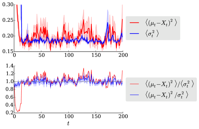
Refer to caption
Figure 5: Posterior variance vs. MSE when filtering a one-dimensional process dXt=0.1Xtdt+0.5dWt𝑑subscript𝑋𝑡0.1subscript𝑋𝑡𝑑𝑡0.5𝑑subscript𝑊𝑡dX_{t}=-0.1X_{t}dt+0.5dW_{t} (the steady-state variance of this process is σ02=1.25superscriptsubscript𝜎021.25\sigma_{0}^{2}=1.25). The top plot shows the MSE and mean posterior variance. The bottom plot shows the ratio of means MSE/ΣtMSEdelimited-⟨⟩subscriptΣ𝑡\mathrm{MSE}/\left\langle\Sigma_{t}\right\rangle and the mean ratio SE/Σtdelimited-⟨⟩SEsubscriptΣ𝑡\left\langle\mathrm{SE}/\Sigma_{t}\right\rangle where SE is the squared error (μtXt)2superscriptsubscript𝜇𝑡subscript𝑋𝑡2\left(\mu_{t}-X_{t}\right)^{2}. Sensory parameters are c=0,σpop2=0.1,σtc2=0.01,λ0=10formulae-sequence𝑐0formulae-sequencesuperscriptsubscript𝜎pop20.1formulae-sequencesuperscriptsubscript𝜎tc20.01superscript𝜆010c=0,\sigma_{\mathrm{pop}}^{2}=0.1,\sigma_{\mathrm{tc}}^{2}=0.01,\lambda^{0}=10. The means were taken across 1000 trials. Shaded areas indicate error estimates obtained as sample standard deviation divided by square root of number of trials.

We also show here variants of the Figures 3 and 4 (Figures 6 and 7, respectively), showing the MSE rather than the variance. The results look similar but noisier, except in Figure 7b for small population variance, where the ADF estimation is poor due to very few spikes occurring.
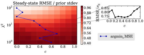
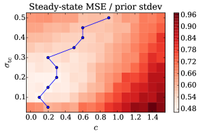
Refer to caption
(a)
Refer to caption
(b)
Figure 6: Mean Square Error as a function of model parameters. This figure is based on the same data as Figure 3, with Root Mean Square Error (RMSE) plotted instead of estimated posterior variance. See Figure 3 for more details.
Refer to caption
(a)
Refer to caption
(b)
Figure 7: Optimal population distribution depends on prior variance relative to tuning curve width. This figure is based on the same data as Figure 4, with MSE plotted instead of estimated posterior variance. See Figure 4 for more details.

References

  • [1] B.D. Anderson and J.B. Moore. Optimal Filtering. Dover, 2005.
  • [2] R.E. Kalman and R.S. Bucy. New results in linear filtering and prediction theory. J. of Basic Eng., Trans. ASME, Series D, 83(1):95–108, 1961.
  • [3] R.E. Kalman. A new approach to linear filtering and prediction problems. J. Basic Eng., Trans. ASME, Series D., 82(1):35–45, 1960.
  • [4] F. Daum. Nonlinear filters: beyond the kalman filter. Aerospace and Electronic Systems Magazine, IEEE, 20(8):57–69, 2005.
  • [5] S. Julier, J. Uhlmann, and H. Durrant-Whyte. A new method for the nonlinear transformation of means and covariances in filters and estimators. IEEE Trans. Autom. Control, 45(3):477–482, 2000.
  • [6] A. Doucet and A.M. Johansen. A tutorial on particle filtering and smoothing: fifteen years later. In D. Crisan and B. Rozovskii, editors, Handbook of Nonlinear Filtering, pages 656–704. Oxford, UK: Oxford University Press, 2009.
  • [7] P. Brémaud. Point Processes and Queues: Martingale Dynamics. Springer, New York, 1981.
  • [8] D.L. Snyder and M.I. Miller. Random Point Processes in Time and Space. Springer, second edition edition, 1991.
  • [9] P. Dayan and L.F. Abbott. Theoretical Neuroscience: Computational and Mathematical Modeling of Neural Systems. MIT Press, 2005.
  • [10] O. Bobrowski, R. Meir, and Y.C. Eldar. Bayesian filtering in spiking neural networks: noise, adaptation, and multisensory integration. Neural Comput, 21(5):1277–1320, May 2009.
  • [11] Y. Ahmadian, J.W. Pillow, and L. Paninski. Efficient markov chain monte carlo methods for decoding neural spike trains. Neural Comput, 23(1):46–96, Jan 2011.
  • [12] A.K. Susemihl, R. Meir, and M. Opper. Analytical results for the error in filtering of gaussian processes. In J. Shawe-Taylor, R.S. Zemel, P. Bartlett, F.C.N. Pereira, and K.Q. Weinberger, editors, Advances in Neural Information Processing Systems 24, pages 2303–2311. 2011.
  • [13] A.K. Susemihl, R. Meir, and M. Opper. Dynamic state estimation based on poisson spike trains—towards a theory of optimal encoding. Journal of Statistical Mechanics: Theory and Experiment, 2013(03):P03009, 2013.
  • [14] P.S. Maybeck. Stochastic Models, Estimation, and Control. Academic Press, 1979.
  • [15] D. Brigo, B. Hanzon, and F. LeGland. A differential geometric approach to nonlinear filtering: the projection filter. Automatic Control, IEEE Transactions on, 43:247–252, 1998.
  • [16] M. Opper. A Bayesian approach to online learning. In D. Saad, editor, Online Learning in Neural Networks, pages 363–378. Cambridge university press, 1998.
  • [17] T.P. Minka. Expectation propagation for approximate bayesian inference. In Proceedings of the Seventeenth conference on Uncertainty in artificial intelligence, pages 362–369. Morgan Kaufmann Publishers Inc., 2001.
  • [18] N.S. Harper and D. McAlpine. Optimal neural population coding of an auditory spatial cue. Nature, 430(7000):682–686, Aug 2004. n1397b.
  • [19] M. Bethge, D. Rotermund, and K. Pawelzik. Optimal short-term population coding: when fisher information fails. Neural Comput, 14(10):2317–2351, Oct 2002.
  • [20] S. Yaeli and R. Meir. Error-based analysis of optimal tuning functions explains phenomena observed in sensory neurons. Front Comput Neurosci, 4:130, 2010.
  • [21] D. Ganguli and E.P. Simoncelli. Efficient sensory encoding and bayesian inference with heterogeneous neural populations. Neural Comput, 26(10):2103–2134, 2014.
  • [22] D.L. Snyder and M.I. Miller. Random Point Processes in Time and Space. Springer, second edition edition, 1991.
  • [23] I. Rhodes and D. Snyder. Estimation and control performance for space-time point-process observations. IEEE Transactions on Automatic Control, 22(3):338–346, 1977.
  • [24] A.K. Susemihl, R. Meir, and M. Opper. Optimal Neural Codes for Control and Estimation. Advances in Neural Information Processing Systems, pages 1–9, 2014.
  • [25] D. Snyder. Filtering and detection for doubly stochastic Poisson processes. IEEE Transactions on Information Theory, 18(1):91–102, January 1972.
  • [26] A. Brand, O. Behrend, T. Marquardt, D. McAlpine, and B. Grothe. Precise inhibition is essential for microsecond interaural time difference coding. Nature, 417(6888):543–547, 2002.