Photons emerging as Goldstone bosons from spontaneous Lorentz symmetry breaking: The Abelian Nambu model

Abstract

After imposing current conservation together with the Gauss law as initial conditions on the Abelian Nambu model, we prove that the resulting theory is equivalent to standard QED in the non-linear gauge $\left(A_{\mu}A^{\mu}-n^{2}M^{2}\right)=0$, to all orders in perturbation theory. We show this by writing both models in terms of the same variables, which produce identical Feynman rules for the interactions and propagators. A crucial point is to verify that the Faddeev-Popov ghosts arising from the gauge fixing procedure in the QED sector decouple to all orders. We verify this decoupling by following a method like that employed in Yang-Mills theories when investigating the behavior of axial gauges. The equivalence between the two theories supports the idea that gauge particles can be envisaged as the Goldstone bosons originating from spontaneous Lorentz symmetry breaking.

I Introduction

The Abelian Nambu model (ANM) was proposed in Ref. Nambu-Progr to describe electrodynamics in a way similar to the construction of pion interactions in the nonlinear sigma model characterized by spontaneous chiral symmetry breaking. The understanding of pions as the Goldstone bosons (GB) arising from such breaking motivated the possibility of looking at photons as the GB resulting from a spontaneous Lorentz symmetry breaking (SLSB). The ANM is defined by the Lagrangian density

$$\mathcal{L}=-\frac{1}{4}F_{\mu\nu}F^{\mu\nu}-J_{\mu}A^{\mu},\;\;$$ (1)

plus the non-linear constraint

$$A_{\mu}A^{\mu}-n^{2}M^{2}=0,\;\;\;\;\;\;\;\;M>0.$$ (2)

The vector $n^{\mu}$ signals the direction of the non-zero vacuum expectation value $\langle A^{\mu}\rangle=n^{\mu}M$ inducing the SLSB. Usually, one deals separately with the three characteristic cases dictated by the choice of the vector $n^{\mu}$ as time-like $(n^{2}>0)$, space-like $(n^{2}<0)$ or light-like $(n^{2}=0)$. Here we consider only the first two options where a natural choice of independent degrees of freedom (DOF) is the following

$$n^{2} > 0:\quad A_{1},\;A_{2},\;A_{3},\qquad\rightarrow\qquad A_{0}=\sqrt{M^{2}+A_{i}A_{i}},\qquad i=1,2,3,$$ (3)

$$n^{2} < 0:\quad A_{0},\;A_{1},\;A_{2},\qquad\rightarrow\qquad A_{3}=\sqrt{M^{2}+A_{0}A_{0}-A_{a}A_{a}},\qquad a=1,2.$$ (4)

The solutions of the constraint (2) shown in Eqs. (3) and (4) make clear the symmetry breaking from $SO(1,3)$ to $SO(3)$ and from $SO(1,3)$ to $SO(2,1)$ in the time-like and space-like cases, respectively. Each realization of the ANM is defined by substituting the dependent variable into the standard Lagrangian density for electrodynamics (1). The calculation of some particular processes in perturbation theory demand a further expansion of the non linear terms in the resulting Lagrangian density in powers of the combinations $\left(A_{i}A_{i}\right)/M^{2}$ (time-like case) and $\left(A_{0}A_{0}-A_{a}A_{a}\right)/M^{2}$ (space-like case). After the solutions (3) and (4) of the constraint are inserted in the Lagrangian density (1) one ends up with a regular system having three DOF per point in coordinate space, where the resulting equations of motion are different from Maxwell’s equations Nambu-Progr ; Urru-Mont .

Nambu models have been further studied in relation to electrodynamics Urru-Mont ; VENT1 ; Azatov-Chkareuli and also have been generalized to the non-abelian VENT2 ; JLCH1 ; JLCH2 ; JLCH3 and gravitational cases JLCH4 . Quantum electrodynamics in the nonlinear gauge (2) is considered in Refs. VENT1 . General conditions on how the gauge symmetries are recovered from models that involve SLSB are worked out in Refs. RUSOS ; JLCH5 ; JLCH6 ; JLCH7 . In particular, the result obtained in Refs. Nambu-Progr ; Urru-Mont ; NANM_ES_UR states that the dynamics of the ANM guarantees the validity of the Gauss Law for all times, once the Gauss law and current conservation are imposed as initial conditions. In this way, after demanding such initial conditions, the ANM reduces to electrodynamics and current conservation remain valid for all times as the consequence of the restored gauge invariance.

An alternative way of exploring the connection between gauge theories and models with SLSB is by means of the so-called bumblebee models appearing in the study of possible observable violations of Lorentz invariance Colladay-Kostelecky . These models introduce GB modes and depending on the explicit form of the theory they present additional massive modes and constraints. Such models have been thoroughly investigated in relation to electrodynamics BLUHM_1 ; HERNASKI and gravity BLUHM_3 ; BLUHM_2 ; KOS_POT ; CARROLL .

In this work we consider the relation between the ANM and standard QED from a perturbative perspective, paying attention to the gauge fixing procedure that is required in QED to study their equivalence. Perturbative calculations in the ANM show that, to the order considered (tree level and one-loop diagrams), all SLSB contributions to physical processes cancel out, yielding the same results as in standard QED Nambu-Progr ; Azatov-Chkareuli . This feature has been interpreted by stating that the non-linear constraint (2) can be seen just as a gauge choice in QED, which would then explain why the two theories are equal. Nevertheless, this statement requires some qualifications: (i) on one hand, the number of degrees of freedom (DOF) of the ANM is three, in such a way that the possible equivalence between both theories requires at least to specify some additional condition to cut this extra DOF. (ii) on the other hand, fixing the gauge in any gauge theory requires the introduction of ghost particles, via the BRST procedure for example, which play a fundamental role as internal particles in calculating physical processes BRST . Thus, to show the proposed equivalence one would need to study their contributions. A possible decoupling of such ghosts is by no means clear, especially due to the non-linear character of the suggested gauge fixing.

The paper is organized as follows. In section 2 we review some basic points of the perturbative calculation presented in Ref. Azatov-Chkareuli , where the authors introduce a convenient field redefinition $A_{\mu}\rightarrow a_{\mu}$, which allows to write the ANM in terms of the GB modes only. This formulation serves as the benchmark for the comparison of the ANM with QED. Section 3 describes how the BRST formalism fixes the gauge $A_{\mu}A^{\mu}=n^{2}M^{2}$ in QED, introducing the required Faddeev-Popov ghosts (FPG). The resulting gauge fixed QED Lagrangian density is then written in terms of the same field redefinition $A_{\mu}\rightarrow a_{\mu}$ already introduced in section 2. In this way, one can show that the Feynman amplitudes for physical processes arising from the ANM Lagrangian density and those stemming form the gauge fixed QED Lagrangian density differs only by the contributions from the Feynman diagrams including the FPG interactions. The ghost propagator, together with the other Feynman rules, is calculated in section 4. Finally, section 5 includes the general perturbative proof on how the ghosts decouple when QED is formulated in the gauge fixed Lagrangian density found in section 3. In section 6 we close with a summary, where we put together all the pieces which prove the perturbative equivalence between the two models.

II The perturbative formulation of the ANM

In this section, we summarize the approach of Ref. Azatov-Chkareuli , which is appropriate to make explicit the relation between the ANM and QED to be established in the following.

The starting point in Ref. Azatov-Chkareuli is the standard fermionic QED Lagrangian density

$$\mathcal{L}_{\mathrm{QED}}(A_{\mu},{\bar{\psi}},\psi)=\mathcal{-}\frac{1}{4}F_{\mu\nu}F^{\mu\nu}+\bar{\psi}\left(i\gamma\partial+m\right)\psi-eA_{\mu}\bar{\psi}\gamma^{\mu}\psi,$$ (5)

plus the constraint (2), where the authors then introduce a very useful parameterization in terms of the new field $a_{\mu}$, by defining

$$A_{\mu}(a_{\rho})=a_{\mu}+\frac{n_{\mu}}{n^{2}}(M^{2}-n^{2}a^{2})^{1/2},\quad\;n^{2}\neq 0.$$ (6)

This transformation can be inverted yielding

$$a_{\mu}=A_{\mu}-\frac{n_{\mu}}{2n^{2}}\left(\left(n\cdot A\right)+\sqrt{\left(n\cdot A\right)^{2}+2\left(M^{2}-A^{2}n^{2}\right)}\right).$$ (7)

When we substitute (6) into (5) we get $\mathcal{L}_{\mathrm{QED}}(A_{\mu}(a_{\nu}),{\bar{\psi}},\psi)$, which is a highly non-linear expression in terms of the new field$\;a_{\mu}.\;$Nevertheless,$\;\mathcal{L}_{\mathrm{QED}}(A_{\mu}(a_{\nu}),{\bar{\psi}},\psi)\;$is still a Lagrangian density for QED, written in a very unconventional way, which nevertheless provides a convenient interpretation of the field $a_{\mu}$ once the ANM is defined. Notice that gauge invariance $\delta A_{\mu}=\partial_{\mu}\delta\Lambda\;$remains an invariance of $\;\mathcal{L}_{\mathrm{QED}}(A_{\mu}(a_{\nu}),{\bar{\psi}},\psi)\;$realized in terms of a very complicated transformation $\delta a_{\mu}$, which could be obtained from Eq.  (7). An important property of the field redefinition (6) is the relation

$$\left(A_{\mu}A^{\mu}-n^{2}M^{2}\right)^{2}=4\left(a\cdot n\right)^{2}\left[M^{2}-n^{2}a^{2}\right].$$ (8)

Next, the authors of Ref. Azatov-Chkareuli focus on the ANM, by imposing the non-linear constraint (2) on the Lagrangian density $\mathcal{L}_{\mathrm{QED}}(A_{\mu}(a_{\nu}),{\bar{\psi}},\psi)$. In terms of the new fields $a_{\nu}$, the condition (2) takes the simpler form

$$n\cdot a=0,$$ (9)

according to the relation (8). The fields $a_{\nu}$, satisfying (9), define three DOF that are orthogonal to the vacuum $n^{\mu},$ so that they describe the Goldstone modes of the model.

Since the ANM is defined by solving a constraint involving four fields in terms of three DOF and after substituting the solution in the electromagnetic sector of the model, it is enlightening to compare the two possibilities offered once we introduce the field $a_{\nu}$, to appreciate the advantage of this redefinition. For the time-like case $n^{\mu}=(1,0,0,0)$, the solution $A_{0}=\sqrt{M^{2}+A_{i}A_{i}}$, together with the choice of $A_{i}$ as the independent variables is fully equivalent to set $a_{0}=0$ and recognize that $a_{i}=A_{i}$. For the space-like case $n^{\mu}=(0,0,0,1)$ the choice of independent variables $A_{0},A_{a}$, together with the definition $A_{3}=\sqrt{M^{2}+A_{0}A_{0}-A_{a}A_{a}}$, corresponds to set $a_{3}=0,a_{0}=A_{0}\;$and $a_{a}=A_{a}$. Thus, the substitution of $A_{0}$ or $A_{3}$ into (5), according to the choices (3) or (4), is equal to the introduction of the field redefinition (6) with the proper choice of $n^{\mu}$, which we can select at the end of the calculation. This provides a unified method of dealing with the time-like and space-like cases. Consequently, and following Ref. Azatov-Chkareuli , we can write the Lagrangian density for the cases of interest in the ANM as

$$\mathcal{L}_{\mathrm{ANM}}(a_{\mu},{\bar{\psi}},\psi)=\mathcal{L}_{\mathrm{QED}}(A_{\mu}(a_{\nu}),{\bar{\psi}},\psi),\;\;\;n\cdot a=0.\;$$ (10)

The constraint (9) clearly breaks gauge invariance together with active Lorentz invariance. The field redefinition $A_{\mu}(a_{\rho})$ implies that we have to substitute

$$F_{\mu\nu}=f_{\mu\nu}+\frac{1}{n^{2}}\left(n_{\nu}\partial_{\mu}-n_{\mu}\partial_{\nu}\right)(M^{2}-n^{2}a^{2})^{1/2},\;\;\;f_{\mu\nu}=\partial_{\mu}a_{\nu}-\partial_{\nu}a_{\mu},\;\;\;$$ (11)

for the field strength $F_{\mu\nu}$ in (5).

The next step in Ref. Azatov-Chkareuli is to make an expansion of $\mathcal{L}_{\mathrm{QED}}(A_{\mu}(a_{\nu}),{\bar{\psi}},\psi)$ in powers of $a^{2}/M^{2}$ keeping terms up to the order $(a^{2})^{2}/M^{2}$, which defines the Lagrangian density of the ANM to the order considered in that reference. The corresponding Feynman rules are given in Ref. Azatov-Chkareuli and we recall here the GB propagator $D_{\mu\nu}^{\mathrm{ANM}}(k)$ which we will need in the following

$$D_{\mu\nu}^{\mathrm{ANM}}(k)=-\frac{i}{k^{2}+i\epsilon}\left[\eta_{\mu\nu}-\frac{n_{\mu}k_{\nu}+n_{\nu}k_{\mu}}{\left(n\cdot k\right)}+\frac{n^{2}k_{\mu}k_{\nu}}{\left(n\cdot k\right)^{2}}\right],\;\;\;n^{\mu}D_{\mu\nu}^{\mathrm{ANM}}=0\;.$$ (12)

We remind the reader that the authors of Refs. Nambu-Progr ; Azatov-Chkareuli have shown that the extra contributions to some specific QED processes (up to one loop order), arising from the Lorentz violating terms in the Lagrangian density (10) exactly cancel in the ANM calculation, thus yielding the standard QED results.

Let us emphasize that the perturbative calculation naturally incorporates the two initial conditions required for the equivalence between the ANM and QED, which are the imposition of the Gauss law together with current conservation Nambu-Progr ; Urru-Mont ; NANM_ES_UR . The Lagrangian density of the ANM in the interaction picture starts with the free contribution

$$\mathcal{L}_{0}(a_{\mu},{\bar{\psi}},\psi)=\mathcal{-}\frac{1}{4}f_{\mu\nu}f^{\mu\nu}+\bar{\psi}\left(i\gamma\partial+m\right)\psi,\;\;\;\;n\cdot a=0,\;$$ (13)

which describes the behavior of the system at $t\;\rightarrow-\infty$. The electric current $J^{\mu}=e\bar{\psi}\gamma^{\mu}\psi$ is conserved, as it is the Noether current arising from the invariance under global phase transformations of the fermionic fields in the Lagrangian density (13). Also, the Lagrangian density (13) yields the GB propagator (12), which satisfies the on-shell condition  $k^{\mu}D_{\mu\nu}^{\mathrm{ANM}}=0$, for $k^{2}=0$. That is to say, the Gauss law has been implemented à la Dirac upon the initial physical states, by imposing the transversality condition $k^{\mu}\epsilon_{\mu}(k)=0$ on the external GB modes having the polarization vectors $\epsilon_{\mu}(k)$. Both conditions play a crucial role in the cancellations obtained in Ref. Azatov-Chkareuli , which suggest the equivalence, to this order in perturbation theory, between QED and the ANM with appropriate initial conditions.

III Electrodynamics in the gauge $A_{\mu}A^{\mu}=n^{2}M^{2}$

Now we switch to electrodynamics. The main point we address in this section is the behavior of the Faddeev-Popov ghost (FPG) interactions that will necessarily appear when fixing the proposed gauge. We move forward after the basic prescription of the BRST method BRST , applied to the QED the Lagrangian density (5), which is invariant under the gauge transformations $\delta A_{\mu}=\partial_{\mu}\Lambda$. First we introduce the fermionic nilpotent transformation $\tilde{\delta}$, together with the new fields $c,\;\bar{c}$ and $b$ in such a way that

$$\tilde{\delta}A_{\mu}=\partial_{\mu}c,\qquad\tilde{\delta}c=0,\qquad\tilde{\delta}\bar{c}=ib,\qquad\tilde{\delta}b=0.$$ (14)

Next we construct the BRST invariant Lagrangian density

$$\mathcal{L}_{\mathrm{BRST}}=-\frac{1}{4}F_{\mu\nu}F^{\mu\nu}+i\tilde{\delta}\left[\bar{c}\left(\left(A_{\mu}A^{\mu}-n^{2}M^{2}\right)+\frac{b}{2\alpha}\right)\right],$$ (15)

where we have explicitly introduced the gauge fixing condition. Performing the $\tilde{\delta}$ variation and eliminating $b$ from its algebraic equation of motion, we get the Lagrangian density

$$\mathcal{L}_{\mathrm{BRST}}=-\frac{1}{4}F_{\mu\nu}F^{\mu\nu}-\frac{\alpha}{2}\left(A_{\mu}A^{\mu}-n^{2}M^{2}\right)^{2}-2A^{\mu}i\bar{c}\partial_{\mu}c,$$ (16)

which clearly exhibits $\,\alpha\left(A_{\mu}A^{\mu}-n^{2}M^{2}\right)^{2}/2\,$ as the gauge fixing term and brings in the FPG $c$ and $\bar{c}$, which are independent real Grassman numbers. At this stage it is convenient to introduce also the parameterization (6) for the photon field $A^{\mu}$. Recalling that such parameterization yields the exact result (8), the final gauge fixed Lagrangian density for QED is

$$\mathcal{L}_{\mathrm{GFED}} = \mathcal{L}_{\mathrm{QED}}(A_{\mu}(a_{\nu}),{\bar{\psi}},\psi)$$ (17)

$$-2\alpha M^{2}\left(n\cdot a\right)^{2}+2\alpha n^{2}a^{2}\left(n\cdot a\right)^{2}$$

$$-2\left(a^{\mu}+\frac{n^{\mu}}{n^{2}}(M^{2}-n^{2}a^{2})^{1/2}\right)i\bar{c}\partial_{\mu}c,$$

where we have only added the gauge fixing contributions to the Lagrangian density $\mathcal{L}_{\mathrm{QED}}(A_{\mu}(a_{\nu}),{\bar{\psi}},\psi)$. Let us emphasize that $\mathcal{L}_{\mathrm{QED}}(A_{\mu}(a_{\nu}),{\bar{\psi}},\psi)$ appearing in Eq. (17) is the same Lagrangian density which defines the ANM in Eq. (10). Notice that the gauge fixing term reduces to $2\alpha M^{2}\left(n\cdot a\right)^{2}$, when written in terms of the redefined photon field $a_{\mu}$. This corresponds to the choice of an axial gauge in electrodynamics, but with added Yang-Mills type interactions. That is to say, the field $a^{\mu}$ now describes photons in the gauge $\left(n\cdot a\right)=0$, instead of GB modes as in the previous section. From Ref. LEIBBRANDT we read the photon propagator in the axial gauge

$$D_{\mu\nu}^{\mathrm{QED}}(k)=\frac{-i}{k^{2}+i\epsilon}\left[\eta_{\mu\nu}-\frac{k_{\mu}n_{\nu}+n_{\mu}k_{\nu}}{\left(n\cdot k\right)}+k_{\mu}k_{\nu}\frac{n^{2}+\frac{k^{2}}{4\alpha M^{2}}}{\left(n\cdot k\right)^{2}}\right],$$ (18)

satisfying

$$k^{\mu}D_{\mu\nu}^{\mathrm{QED}}(k)=0,\qquad n^{\mu}D_{\mu\nu}^{\mathrm{QED}}(k)=\frac{-i}{k^{2}+i\epsilon}\left[\frac{k^{2}k_{\nu}}{4M^{2}\left(n\cdot k\right)}\right]\frac{1}{\alpha}.$$ (19)

Next we choose the so called pure (homogeneous) axial gauge, defined by $\alpha\rightarrow\infty$, and see that the propagator (18) reduces to (12), that is precisely the one employed in the ANM calculation of Ref. Azatov-Chkareuli , which nevertheless arises in QED from the gauge fixing.

The next step in dealing with the contribution to physical processes of the terms in the QED gauge fixed Lagrangian density is to consider the two non-linear terms in the second line of Eq. (17), which do not depend on the FPG and which are not present in the ANM Lagrangian density of Eq. (10). The last term in that line is proportional to $a^{2}\left(n\cdot a\right)^{2}$ and produces a four-photon vertex $V_{\alpha\beta\mu\nu}$

$$V_{\alpha\beta\mu\nu}\sim\alpha(\eta_{\alpha\beta}n_{\mu}n_{\nu}+perm.\;).$$ (20)

When we saturate $V_{\alpha\beta\mu\nu}$ with internal photon lines, via the corresponding propagators, this vertex will have two contractions of the type $n^{\mu}D_{\mu\rho}$ which give a factor $1/\alpha^{2}$. In this way, the net contribution goes like $1/\alpha$ and thus cancels in the limit $\alpha\rightarrow\infty$. On the other hand, for on-shell photons we have $n^{\mu}D_{\mu\nu}(k)=0=k^{\mu}D_{\mu\nu}(k)$ in such a way that their polarizations vectors  $\epsilon_{\mu}(k)$ must satisfy $n^{\mu}\epsilon_{\mu}(k)=0=k^{\mu}\epsilon_{\mu}(k)$. These added conditions lead also to a zero contribution when we attach external photons to $V_{\alpha\beta\mu\nu}$. The same argument applies to the gauge fixing term proportional to $\left(n\cdot a\right)^{2}$. In other words, the terms proportional to $\left(n\cdot a\right)$ just carry out the gauge condition $\left(n\cdot a\right)=0$.

Then, in the pure axial gauge, the gauge fixed Lagrangian density ${\mathcal{L}_{\mathrm{GFED}}}$ for fermionic electrodynamics, in the parameterization of Ref. Azatov-Chkareuli , reads

$$\mathcal{L}_{\mathrm{GFED}}=\mathcal{L}_{\mathrm{QED}}(A_{\mu}(a_{\nu}),{\bar{\psi}},\psi)+\mathcal{L}_{\mathrm{GHOST}},$$ (21)

which we compare with the ANM Lagrangian density in Eq. (10). In both cases the requirement $\left(n\cdot a\right)=0$ holds, however for different reasons: it is a defining condition in the ANM, while it corresponds to a gauge fixing condition in QED. Let us recall that the field $a_{\mu}\;$has the same propagator in both theories, as seen from  Eq. (12) for the ANM and from the limit $\alpha\rightarrow\infty$ in Eq. (18) for QED. In this way, the condition $\left(n\cdot a\right)=0$ is implemented in the same way for each model in terms of the Feynman rules for the $a_{\mu}$ propagator. This propagator also imposes the Gauss law as an initial condition in the ANM by demanding transversality of the on-shell GB. Besides, as already mentioned, the perturbative expansion in terms of fields in the interaction picture guarantees current conservation as an initial condition in the ANM. Moreover, the remaining Feynman rules for the fields $a_{\mu},{\bar{\psi}},\psi$, which arise from $\mathcal{L}_{\mathrm{QED}}(A_{\mu}(a_{\nu}),{\bar{\psi}},\psi)$, are the same in both cases. In this way, the only difference between the perturbative expansions of the ANM and the gauge fixed QED arises from the ghost interactions

$$\mathcal{L}_{\mathrm{GHOST}}=-2\left(a^{\mu}+\frac{Mn^{\mu}}{n^{2}}\left(1-\frac{n^{2}a^{2}}{M^{2}}\right)^{1/2}\right)i\bar{c}\partial_{\mu}c,$$ (22)

which contributions we study in the following sections.

IV The Feynman rules for Electrodynamics in the gauge $A_{\mu}A^{\mu}=n^{2}M^{2}$

In this section we find the extra Feynman rules arising from the FPG couplings to the photon in the gauge-fixed QED. Since $\bar{c}$ and $c$ are two independent real Grassman fields we find it more convenient to introduce the real doublet

$$\left[\begin{array}[]{c}c\\ \bar{c}\end{array}\right]=\frac{1}{\sqrt{2}}\Phi,\qquad\Phi=\Phi^{\ast},$$ (23)

in terms of which we can write

$$i\bar{c}\partial_{\mu}c=\frac{i}{4}\Phi\sigma^{(1)}\partial_{\mu}\Phi-\frac{i}{2}\partial_{\mu}(c{\bar{c}}),\qquad\sigma^{(1)}=\left[\begin{array}[]{cc}0&1\\ 1&0\end{array}\right]=(\sigma^{(1)})^{T}.$$ (24)

To get the ghost Feynman rules we need to expand Eq. (22) in powers of $n^{2}a^{2}/M^{2}$, in the same way as done for the ANM. We get

$$\hskip-19.91684pt\mathcal{L}_{\mathrm{GHOST}}=-\frac{Mn^{2}}{2}\Phi\sigma^{(1)}\left(n\cdot i\partial\right)\Phi-a^{\mu}\Phi\sigma^{(-)}i\partial_{\mu}\Phi+$$

$$\hskip-19.91684pt+\left(\Phi\sigma^{(-)}\left(n\cdot i\partial\right)\Phi\right)\sum_{m=1}\left(\frac{(2m-3)!!}{2^{m}m!}\right)\left(\frac{\left((n^{\mu}n_{\mu})\right)^{m-1}}{M^{2m-1}}\right)\left(a^{2}\right)^{m},$$ (25)

where we have substituted Eq. (24) and omitted a total derivative. We have rewritten the ghost-photon interaction in terms of the field $\Phi$ by introducing $\sigma^{(-)}=(\sigma^{(1)}-i\sigma^{(2)})/2$, where $\sigma^{(2)}$ is the standard Pauli matrix. We indicate the Feynman rules for the FPG obtained from (25) in the following figures. Dashed lines denote the FPG and wavy lines denote the photon. Figure 1 shows the FPG propagator, which arises from the kinetic term in Eq. (25). Figure 2 shows the vertex $V^{1}$ describing the ghost-photon interaction. Figure 3 shows the vertices ${V}^{2m},m=1,2,\cdots$ describing the ghost-($2m$ photons) interaction. The function $V_{\alpha_{1}\beta_{1}\alpha_{2}\beta_{2}....\alpha_{m}\beta_{m}}$ is independent of the momenta and it is given by

$$V_{\alpha_{1}\beta_{1}\alpha_{2}\beta_{2}....\alpha_{m}\beta_{m}}=\frac{\left(n^{2}\right)^{m-1}(2m-3)!!}{M^{2m-1}}\left(\eta_{\alpha_{1}\beta_{1}}\eta_{\alpha_{2}\beta_{2}}.....\eta_{\alpha_{m}\beta_{m}}+perm\right).$$ (26)

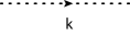
Figure 1: The ghost propagator: $s(k)=\sigma^{(1)}\frac{i}{M}\frac{n^{2}}{(n\cdot k)}$.

The permutations in Eq.(26) do not include repetitions and there are $(2m)!/(2^{m}m!)$ terms for a given $m$. We suppress tensor indices in the notation $V^{1}$ and ${V}^{2m}$, which can be recovered from the definitions in Figure 2 and Figure 3, together with Eq.(26).

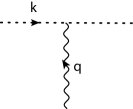
Figure 2: The ghost-photon vertex: $V^{1}(k^{\mu})=\sigma^{(-)}\frac{i}{2}k^{\mu}$.

V Faddeev-Popov Ghosts contributions to physical processes

Finally, we consider the extra Feynman amplitudes to physical processes arising from the FPG interactions. Since FPG couple only to the photon, their contribution will appear as internal loops which generic diagram is shown in Figure 4.

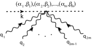
Figure 3: The ghost-($2m$ photons) vertex: $V^{2m}(k^{\mu})=-\sigma^{(-)}\frac{i}{2}(n\cdot k)\,V_{\alpha_{1}\beta_{1}\alpha_{2}\beta_{2}\dots\alpha_{m}\beta_{m}}$.

This loop has $N$ vertex insertions which can be of two types: one photon vertex $V^{1}(k)$ and $2m$-photons vertex $V^{2m}(k)$. They will be generically denoted by $V^{A}(k_{A}),\;\;A=1,2,4,\cdots,2m,\cdots$, where $k_{A}$ indicates the ghost momentum coming into the corresponding vertex. We keep track of the position of each vertex in the loop by an additional subindex $n$ in $V_{n}^{A_{n}}(k_{A_{n}}),$ where $A_{n}=1,2,\cdots,2m,\cdots$, labels the type of the vertex $n$ and $k_{A_{n}}$ stands for the incoming ghost momentum.

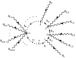
Figure 4: General closed loop ghost diagram with N vertices, showing arbitrary insertions of type $V^{1}$ and type $V^{2m}$. All photons are incoming. The photons arriving to vertices $(N-1)$ and $N$ are not shown.

Each vertex $V^{A}(k_{A})$ has also incoming external photon momenta denoted by $Q_{A}$. For a type $1$ vertex, $Q_{A}$ is just the momentum of the incoming photon, while for a type $2m$ vertex in the $n$-place we have $Q_{A_{n}=2m}=[q_{1,n}+q_{2,n}+\cdots+q_{2m,n}]$, which is the sum of the momenta of the $2m$ incoming photons. The basic unit forming the loop is the product of the propagator  $s_{n}^{A_{n}}(k_{A_{n}})\;\$corresponding to the ghost coming into each vertex, times the corresponding vertex factor$\;V_{n}^{A_{n}}(k_{A_{n}})$, which results in $s_{n}^{A_{n}}(k_{A_{n}})\times V_{n}^{A_{n}}(k_{A_{n}})$. Let us denote $k_{A_{1}}=k$ the momentum entering the first ($n=1$) vertex $V_{1}^{A_{1}}$, which will serve as the integration variable over the loop. Without writing the external connections of the photons entering each vertex and using dimensional regularization, we find that a ghost loop with $N$ vertices contributes to the amplitude with

$$iM_{L} \sim \int\frac{d^{D}k}{(2\pi)^{D}}Tr\left(\left[s_{1}^{A_{1}}(k_{A_{1}}=k)V_{1}^{A_{1}}(k_{A_{1}})\right]\left[s_{2}^{A_{2}}(k_{A_{2}})V_{2}^{A_{2}}(k_{A_{2}})\right]\right.$$ (27)

$$\left.\times.......\times\left[s_{n}^{A_{n}}(k_{A_{n}})V_{n}^{A_{n}}(k_{A_{n}})\right]......\left[s_{N}^{A_{N}}(k_{A_{N}})V_{N}^{A_{N}}(k_{A_{N}})\right]\right).$$

We have

$$k_{A_{\left(n+1\right)}}=Q_{A_{n}}+k_{A_{n}},\quad k_{A_{1}}=k,\quad k_{A_{n}}=k+Q_{A_{1}}+\cdots+Q_{A_{\left(n-1\right)}}.$$ (28)

Here, $Q_{A_{n}}$ are the total external photon momenta entering the loop through the vertex $n$,  satisfying$\;\;\sum_{n=1}^{N}Q_{A_{n}}=0$, so that the ghost momentum after the vertex $N$ is equal to $k=k_{A_{1}}$. The loop has $N$ vertices and $N$ propagators, each contributing with a matrix factor $\sigma^{(-)}$ and $\sigma^{(1)}$, respectively. In this way, the trace corresponds to $Tr\left((\sigma^{(-)}\sigma^{(1)})^{N}\right)=1$.

Some important simplifications occur due to the specific form of the ghost propagator and the ghost-($2m$ photons) vertex. In fact, when the $r$ vertex is of type $2m$, the dependence on the factor $n\cdot(k_{A_{r=2m}})$ in the vertex cancels with that of the propagator, yielding the momentum independent contribution

$$s_{r}^{A_{r}=2m}(k_{A_{r}=2m})V_{r}^{A_{r}=2m}(k_{A_{r}=2m})=\left(\frac{1}{2M^{2}}\right)V_{\alpha_{1}\beta_{1}\cdots\alpha_{m}\beta_{m}},$$ (29)

that can be taken out of the $d^{D}k$ integration and which is not written in the following steps.

In this way, we are left with contributions to the diagram arising only from vertices of type $1$, together with the respective propagators. Thus, we have

$$iM_{L} \sim \int\frac{d^{D}k}{(2\pi)^{D}}Tr\left(\Pi_{a=1}^{N_{1}}\left[\left(\sigma^{(1)}\frac{i}{M}\frac{n^{2}}{(n\cdot k_{a})}\right)\left(\sigma^{(-)}\frac{i}{2}k_{a}^{\mu_{a}}\right)\right]\right)$$

$$iM_{L} \sim \left(-\frac{n^{2}}{2M}\right)^{N_{1}}\int\frac{d^{D}k}{(2\pi)^{D}}\frac{k_{1}^{\mu_{1}}k_{2}^{\mu_{2}}...k_{N_{1}}^{\mu_{N_{1}}}}{(n\cdot k_{1})(n\cdot k_{2})...(n\cdot k_{N_{1}})},$$ (30)

where $a=1,\cdots,N_{1}$ relabels the remaining $N_{1}$ type $1$ vertices. Let us denote $k_{a}=k+R_{a}$, where $R_{a}$ is the sum of all the external photon momenta that have entered the loop before the vertex $a$ and after the vertex $1$. Using the standard Feynman’s parameterization for the denominators,

$$\frac{1}{\left[n\cdot(k+R_{1})\right]...\left[n\cdot(k+R_{N_{1}})\right]}=\int_{0}^{1}d\alpha_{1}\cdots d\alpha_{N_{1}}\delta(\alpha_{1}+\cdots+\alpha_{N_{1}}-1)\frac{(N_{1}-1)!}{\left[n\cdot\left(k+V\left(\alpha\right)\right)\right]^{N_{1}}},$$ (31)

with $V\left(\alpha\right)=\sum_{a=1}^{N_{1}}\alpha_{a}R_{a}$, the contribution from Eq.(30) reduces to

$$iM_{L}\sim\int\frac{d^{D}k}{(2\pi)^{D}}\left(k+S_{1}(\alpha)\right)^{\mu_{1}}\left(k+S_{2}(\alpha)\right)^{\mu_{2}}\left(k+S_{N_{1}}(\alpha)\right)^{\mu_{N_{1}}}\frac{1}{\left(n\cdot k\right)^{N_{1}}}.$$ (32)

Here $S_{a}(\alpha)=R_{a}-V\left(\alpha\right)$. Also, we have made the shift $k+V\left(\alpha\right)\rightarrow k$ in the integration variable of Eq. (30). In Eq. (32) we have omitted the integrations with respect to the Feynman parameters $\alpha_{a}$, which can be taken out of the momentum integral. The numerator in the integral (32) is a linear combination of products of the type

$$k^{\nu_{1}}k^{\nu_{2}}\cdots k^{\nu_{L}},\qquad L=0,1,\cdots,N_{1},$$ (33)

multiplied by $M$ constant vectors $S^{\rho_{i}}S^{\rho_{2}}...S^{\rho_{M}}$, in such a way that $M+L=N_{1}$. The set of $L$ indices $\nu_{1},\nu_{2},\cdots,\nu_{L}$ is chosen among the $N_{1}$ original ones $\mu_{1},\mu_{2},\cdots,\mu_{L},\cdots,\mu_{N_{1}}$, in all possible combinations. Finally, the momentum integral of the ghost loop contributes with a sum of integrals of the form

$$I^{{\nu_{1}\nu_{2}}\cdots{\nu_{L}}}=\int\frac{d^{D}k}{(2\pi)^{D}}\frac{k^{\nu_{1}}k^{\nu_{2}}\cdots k^{\nu_{L}}}{\left(n\cdot k\right)^{N_{1}}},\quad L\leq N_{1},$$ (34)

each of them multiplied by a corresponding $k$-independent tensor. The calculation of such integrals in dimensional regularization has been previously discussed in references such as FRENKEL ; MATSUKI ; LEIBBRANDT . We briefly quote the results of Eqs.(2.5), (2.6) and (2.7) in Ref. MATSUKI . There, the author writes $I^{{\nu_{1}\nu_{2}}\cdots{\nu_{L}}}$ as

$$I^{{\nu_{1}\nu_{2}}\cdots{\nu_{L}}}\sim\frac{\partial}{\partial n_{\nu_{1}}}\frac{\partial}{\partial n_{\nu_{2}}}...\frac{\partial}{\partial n_{\nu_{L}}}\int\frac{d^{D}k}{(2\pi)^{D}}\frac{1}{\left(n\cdot k\right)^{(N_{1}-L)}},$$ (35)

where the basic integral yields

$$\int\frac{d^{D}k}{(2\pi)^{D}}\frac{1}{\left(n\cdot k\right)^{r}}=0,\;\;for\;r>0.$$ (36)

He considers separately the case $r=0,\;(L=N_{1})$, starting from

$$I^{{\nu_{1}\nu_{2}}...{\nu_{N_{1}}}}\sim\frac{\partial}{\partial n_{\nu_{1}}}\frac{\partial}{\partial n_{\nu_{2}}}...\frac{\partial}{\partial n_{\nu_{(N_{1}-1)}}}\int\frac{d^{D}k}{(2\pi)^{D}}\frac{k^{\nu_{N_{1}}}}{\left(n\cdot k\right)}$$ (37)

and calculates the remaining integral assuming $\left(n\cdot k\right)\rightarrow\left(n\cdot k\right)\pm i\epsilon$, obtaining also a zero result.

In this way, using dimensional regularization, we have established that the ghosts decouple when we write QED in the non-linear gauge $A_{\mu}A^{\mu}=n^{2}M^{2}$, or equivalently in the axial gauge $n\cdot a=0\;$plus added nonlinear interactions.

VI Summary

We prove that after imposing the Gauss law and current conservation as initial conditions on the ANM, the resulting theory is equivalent to QED formulated in the non-linear gauge $A_{\mu}A^{\mu}-M^{2}=0$, to all orders in perturbation theory. The strategy is to write both theories in terms of fields describing the same degrees of freedom, which arise from the same Lagrangian density thus yielding identical Feynman rules. In this way, the perturbative calculations of any physical process in each model are indistinguishable.

Our starting point in the fermionic ANM is Ref. Azatov-Chkareuli , where the authors take the useful step of introducing a further field redefinition of $A_{\mu}$ in terms of the variables $a_{\mu}$, which we recall in Eq. (6). In these variables, the constraint $A_{\mu}A^{\mu}-M^{2}=0$ which defines the ANM, translates into the simpler form $\;n\cdot a=0$. This condition exhibits the fields $a_{\mu}$ as the pure GB modes of the model, that are orthogonal to the direction $n_{\mu}$ of the vacuum inducing the SLSB. At this stage, the ANM is defined by the Lagrangian density $\mathcal{L}_{\mathrm{ANM}}(a_{\mu},{\bar{\psi}},\psi)=\mathcal{L}_{\mathrm{QED}}(A_{\mu}(a_{\nu}),{\bar{\psi}},\psi)$, plus the condition $n\cdot a=0$. This condition is a very convenient way of replacing the initial nonlinear constraint because one can make explicit the corresponding substitutions $a_{0}=0$, or $a_{3}=0$ at the end of the calculation, thus allowing for a unified construction of the ANM in the time-like and space-like cases, respectively. The requirement $n\cdot a=0$ is effectively incorporated in the calculations through the propagator $D_{\mu\nu}^{\mathrm{ANM}}(k)$ given in Eq. (12) and satisfying $n^{\mu}D_{\mu\nu}^{\mathrm{ANM}}=0$ together with  $k^{\mu}D_{\mu\nu}^{\mathrm{ANM}}=0$ for on-shell GB. Since the perturbative approach relies on the interaction picture, the fields are quantized starting from the free Lagrangian density (13) which, in particular, leads to the propagator $D_{\mu\nu}^{\mathrm{ANM}}(k)$. As emphasized in Ref. Nambu-Progr , the on-shell transversality of $D_{\mu\nu}^{\mathrm{ANM}}(k)$ guarantees that the Gauss law is imposed, à la Dirac, upon the physical states. Moreover, the free fermionic current is conserved, since it is the Noether current arising from the global phase invariance of the fermionic sector. In this way, the perturbative approach ensures that the two additional requirements to be imposed as initial conditions upon the ANM to recover gauge invariance are indeed satisfied. The remaining Feynman rules are then obtained from the expansion of the Lagrangian density $\mathcal{L}_{\mathrm{ANM}}(a_{\mu},{\bar{\psi}},\psi)=\mathcal{L}_{\mathrm{QED}}(A_{\mu}(a_{\nu}),{\bar{\psi}},\psi)\;$ in powers $a^{2}/M^{2}$.

Next we turn to QED and construct the BRST gauge fixed Lagrangian density, which introduces the Faddeev-Popov ghosts ${\bar{c}},c$. We start from $\mathcal{L}_{\mathrm{QED}}(A_{\mu},{\bar{\psi}},\psi)$ choosing the gauge $A_{\mu}A^{\mu}-M^{2}=0$, but after we rewrite the gauge-fixed Lagrangian density in terms of the same parameterization (6) used in the ANM, observing that now the fields $a_{\mu}$ describe photons instead of Goldstone bosons. The gauge fixing condition $\alpha(A_{\mu}A^{\mu}-M^{2})^{2}$ translates into $4M^{2}\alpha(n\cdot a)^{2}$, which emerges as the choice of an axial gauge, that nevertheless incorporates extra Yang-Mills type interactions. By choosing the pure (homogeneous) axial gauge, $\alpha\rightarrow\infty$, we arrive to the photon propagator $D_{\mu\nu}^{\mathrm{QED}}$ in Eq. (18), which is identical to the ANM propagator $D_{\mu\nu}^{\mathrm{ANM}}$ given in Eq. (12). At this stage, the relation between the two theories, written in terms of the same variables and having the same Feynman rules for the fields $a_{\mu},{\bar{\psi}},\psi$ can be summarized in the following relation between their Lagrangian densities

$$\mathcal{L}_{\mathrm{ANM}}(a_{\mu},{\bar{\psi}},\psi)=\mathcal{L}_{\mathrm{QED}}(A_{\nu}(a_{\mu}),{\bar{\psi}},\psi)+\mathcal{L}_{\mathrm{GHOST}}(a_{\mu},{\bar{c}},c).$$ (38)

In this way, the last step to prove the equivalence between them is to show that the ghosts decouple to all orders in perturbation theory. Following a method similar to that employed in Yang-Mills theories when investigating the behavior of axial gauges, we prove in section 5 that this is indeed the case. We make use of dimensional regularization and we consider the specific photon-ghost interactions of the gauge fixed QED Lagrangian density.

Recapping, because the ghosts decouple, we have shown that the ANM, supplemented by the initial conditions mentioned earlier, together with QED written in the non-linear gauge $A_{\mu}A^{\mu}-M^{2}=0$, are described by the same Lagrangian density $\mathcal{L}_{\mathrm{QED}}(A_{\nu}(a_{\mu}),{\bar{\psi}},\psi)$. This yields to identical Feynman rules for the propagators and the interactions of the common fields $a_{\mu},{\bar{\psi}},\psi$, thus making the two models identical in perturbation theory. The perturbative calculations in Ref. Azatov-Chkareuli constitute detailed examples of this equivalence. Our general result agrees with the Hamiltonian approach discussed in Refs. Urru-Mont ; NANM_ES_UR . As emphasized in such references, to prove the equivalence some additional requirements had to be enforced upon the ANM as initial conditions, which turned out to be valid for all times in virtue of ANM dynamics. These were current conservation and the imposition of the Gauss law upon the physical states. As previously explained in the text, these conditions are fulfilled in the perturbative calculation, which is an expansion in terms of fields in the interaction picture that satisfy free-field equations of motion.

LFU is partly supported by the Project No. IN104815 from Dirección General de Asuntos del Personal Académico (Universidad Nacional Autónoma de México).

References

- (1) Y. Nambu, Suppl. Progr. Theor. Phys. E68, 190 (1968).
- (2) O.J. Franca, R. Montemayor and L.F. Urrutia, Phys. Rev. D 85, 085008 (2012).
- (3) R. Righi and G. Venturi, Int. J. Theor. Phys. 21, 63 (1982); Lett. Nuovo Cim. 31, 487 (1981); Lett. Nuovo Cim. 19, 633 (1977).
- (4) A.T. Azatov and J.L. Chkareuli, Phys. Rev. D 73, 065026 (2006).
- (5) R. Righi, G. Venturi and V. Zamiralov, Nuovo Cim. A47, 518 (1978).
- (6) J. L. Chkareuli and Z. R. Kepuladze, Phys. Lett. B 644, 212 (2007).
- (7) J. L. Chkareuli and J. G. Jejelava, Phys. Lett. B 659, 754 (2008).
- (8) J. L. Chkareuli, C. D. Froggatt and H. B. Nielsen, Nucl. Phys. B 821, 65 (2009).
- (9) J. L. Chkareuli, J. G. Jejelava and G. Tatishvili, Phys. Lett. B 696, 124 (2011).
- (10) E. A. Ivanov and V. I. Ogievetsky, Lett. Math. Phys. 1, 309 (1976).
- (11) J. L. Chkareuli, C. D. Froggatt and H. B. Nielsen, Phys. Rev. Lett. 87, 091601 (2001).
- (12) J. L. Chkareuli, C. D. Froggatt and H. B. Nielsen, Nucl. Phys. B 796, 211 (2008).
- (13) J. L. Chkareuli, C. D. Froggatt and H. B. Nielsen, Nucl. Phys. B 821, 65 (2009).
- (14) For a review see, for example, Proceedings of the First Meeting on CPT and Lorentz Symmetry, Bloomington, IN, 1998, edited by V. A. Kostelecký (World Scientific, Singapore, 1999); Proceedings of the Second Meeting on CPT and Lorentz Symmetry, Bloomington, IN, 2001, edited by V. A. Kostelecký (World Scientific, Singapore, 2001); Proceedings of the Third Meeting on CPT and Lorentz Symmetry, Bloomington, IN, 2004, edited by V. A. Kostelecký (World Scientific, Singapore, 2004); Proceedings of the Fourth Meeting on CPT and Lorentz Symmetry, Bloomington, IN, 2007, edited by V. A. Kostelecký (World Scientific, Singapore, 2007); Proceedings of the Fifth Meeting on CPT and Lorentz Symmetry, Bloomington, IN, 2010, edited by V. A. Kostelecký (World Scientific, Singapore, 2010).
- (15) R. Bluhm, N. L. Gagne, R. Potting and A. Vrublevskis, Phys. Rev. D 77,125007 (2008).
- (16) C. A. Hernaski, Phys. Rev. D 90, 124036 (2014).
- (17) R. Bluhm and V. A. Kostelecký, Phys. Rev. D 71, 065008 (2005).
- (18) R. Bluhm, S. H. Fung and V. A. Kostelecký, Phys. Rev. D 77, 065020 (2008).
- (19) V. A. Kostelecký and R. Potting, Phys. Rev. D 79,065018 (2009).
- (20) S. M. Carroll, H. Tam and I. K. Wehus, Phys. Rev. D 80, 025020 (2009).
- (21) See for example: T. Kugo and S. Uehara, Nucl. Phys. B 197, 378 (1982); D. Nemeschansky, C. Preitschopf and M. Weinstein, Ann. Phys (NY) 183, 226 (1988).
- (22) C. A. Escobar and L. F. Urrutia, Phys. Rev. D 92, 025013 (2015).
- (23) G. Leibbrandt, Rev. Mod. Phys. 59, 1067 (1987).
- (24) J. Frenkel, Phys. Rev. D 13, 2325 (1976).
- (25) T. Matsuki, Phys. Rev. D 19, 2879 (1979).