Congestion management
in traffic-light intersections
via Infinitesimal Perturbation Analysis

Abstract

We present a flow-control technique in traffic-light intersections, aiming at regulating queue lengths to given reference setpoints. The technique is based on multivariable integrators with adaptive gains, computed at each control cycle by assessing the IPA gradients of the plant functions. Moreover, the IPA gradients are computable on-line despite the absence of detailed models of the traffic flows. The technique is applied to a two-intersection system where it exhibits robustness with respect to modeling uncertainties and computing errors, thereby permitting us to simplify the on-line computations perhaps at the expense of accuracy while achieving the desired tracking. We compare, by simulation, the performance of a centralized, joint two-intersection control with distributed control of each intersection separately, and show similar performance of the two control schemes for a range of parameters.

1 Introduction

Infinitesimal Perturbation Analysis (IPA) has been established as a sample-based technique for sensitivity analysis of Discrete Event Dynamic Systems (DEDS). Specifically, it gives formulas or algorithms for the sample derivatives (gradients) of performance functions with respect to structural and control variables. One of its salient features is the simplicity and computational efficiency of its algorithms in a class of DEDS which follow formal rules for propagation of perturbations in a network. Furthermore, the algorithms are based on the monitoring and observation of sample paths associated with the evolving state of the system, and whenever these are measurable in real time, the IPA has a potential in control. For extensive presentations of the IPA technique, please see Ho and Cao (1991); Glasserman (1991); Cassandras and Lafortune (1999).

The principal application-domain of IPA has been in queueing networks. However, in recent years there has been a growing interest in fluid queues and their generalization to a class of Stochastic Hybrid Systems (SHS). There are three reasons for that: (i) the algorithms for IPA often are simpler in the SHS setting than in their DEDS equivalent models; (ii) they often require only an observation of the system’s sample paths but not detailed or explicit knowledge of the underlying probability law and hence may be implementable on-line; and (iii) the IPA derivative estimators are unbiased in a larger class of problems in the SHS framework as compared to the setting of DEDS. Initial developments of IPA in the SHS framework were presented in Cassandras et al. (2002), and more-recent general results as well as surveys can be found in Cassandras et al. (2010); Yao and Cassandras (2011).

We point out that representing a discrete event system by an SHS model may introduce errors in the performance evaluation, and this point was addressed in the aforementioned papers and references therein via simulation-based parameter optimization. In most of these experiments the underlying system that provided the sample paths was a DEDS, but the algorithms for the IPA had been derived from the SHS model. Despite this discrepancy the optimization techniques converged to minimum points (or local minima), thereby suggesting a degree of robustness of them with respect to errors in the computed IPA gradients. This point plays a role in the later developments in this paper, as will be seen in the sequel.

While the principal use of IPA has been in optimization, recently we considered an alternative application in performance regulation. Specifically, we addressed the problem of performance tracking in DEDS with time-varying characteristics. The feedback law we chose is comprised of an integrator with adjustable gain, whose adaptation is based on the IPA derivative of the plant function with respect to the control variable. One of the key issues concerns the robustness of the regulation technique with respect to modeling uncertainties and errors in computing the IPA derivative (Wardi et al. (2015)). An application to throughput regulation in computer processors (Almoosa et al. (2012b)) highlights the importance of this issue since the controller has to run at short cycles, and therefore, if it is robust, it can be designed for simplicity and speed at the expense of accuracy. This approach was justified by simulation results in Almoosa et al. (2012b) as well as an analysis cited therein.

Recently we considered an application of the IPA-based performance regulation technique to congestion management in traffic-light intersections, where the objective was to regulate the queue length in a given direction to a given reference (Wardi and Seatzu (2014)). This paper extends the results therein in the following two ways: It considers vector tracking by a MIMO system while all previous results on IPA-based regulation concerned only SISO systems, and it considers the IPA derivative of a queue length at a given intersection by a control parameter at another intersection. In particular we compare, by simulation, the performance of a joint centralized controller for a two-intersection system with a decentralized control where each intersection is controlled by its own parameter. The results show similar performance for a range of parameters, which indicates the aforementioned robustness of IPA-based control and justifies the use of the simpler, decentralized scheme.

Applications of IPA to road-congestion management have been addressed in Fu and Howell (2003); Panayiotou et al. (2005), and more recently in Geng and Cassandras (2012, 2013, 2015); Fleck and Cassandras (2014). Of course the traffic control problem has been amply researched for decades (see, e.g., Fleck and Cassandras (2014) for a survey of techniques and results), and the IPA approach aims at on-line optimization using sample gradients in conjunction with stochastic approximation. The approach in this paper shares the principle of on-line sample gradients, but deviates from the above-mentioned approach in that it concerns performance regulation (tracking) and not optimization. In particular, it considers the control of queue lengths at traffic lights as a mean of congestion avoidance, and consequently the control laws that we propose are different.

The rest of the paper is is structured as follows. Section 2 summarizes our regulation technique in general terms. Section 3 sets the traffic control problem and analyzes the IPA derivatives, Section 4 provides simulation results, and Section 5 concludes the paper. All of the proofs are relegated to the appendix.

2 Regulation Algorithm: Integral Control with Adaptive Gain

Consider the $n$-dimensional discrete-time control system shown in Figure 1, where $r\in\mbox{$\mathbb{R}$}^{n}$ is the setpoint input vector, $k=1,2,\ldots$, denotes time, $y_{k}\in\mbox{$\mathbb{R}$}^{n}$ is the output vector, $e_{k}\in\mbox{$\mathbb{R}$}^{n}$ is the error signal vector, and $u_{k}\in\mbox{$\mathbb{R}$}^{n}$ is the input to the plant. Suppose first that the plant is a time-varying, memoryless nonlinearity of the form

$$y_{k}=G_{k}(u_{k}),$$ (1)

where $G_{k}:\mbox{$\mathbb{R}$}^{n}\rightarrow\mbox{$\mathbb{R}$}^{n}$, $k=1,2,\ldots$, is called the plant function. Given a reference input vector $r$, the purpose of the control system is to ensure that $\lim_{k\rightarrow\infty}y_{k}=r$. To this end we choose the controller to be a linear system defined as

$$u_{k}\ =\ u_{k-1}+A_{k}e_{k-1},$$ (2)

where $A_{k}\in\mbox{$\mathbb{R}$}^{n\times n}$, and the error signal is defined as

$$e_{k}=r-y_{k}.$$ (3)

Figure 1: Control System

Observe that, if $A_{k}$ is constant independent of $k$, then the above control law essentially is a multi-variable integrator (adder). Integral controllers often are associated with oscillation and narrow stability margins, therefore we chose a variable-gain integrator to extend the stability margins as well as to guarantee performance of the regulation scheme under variations in the plant.

We define $A_{k}$ as

$$A_{k}\ =\left(\frac{\partial G_{k-1}}{\partial u}(u_{k-1})\right)^{-1}.$$ (4)

Equations (1) – (4), computed cyclically in the order $(4)\rightarrow(2)\rightarrow(1)\rightarrow(3)$, define the dynamics of the closed-loop system.

The rationale behind the choice of $A_{k}$ in equation (4) can be seen in the fact that, if the plant is time-invariant and hence $G_{k}(u)=G(u)$, this control law effectively implements the Newton-Raphson method for solving the equation $G(u)=r$. This observation was used in Almoosa et al. (2012a) for the single-variable control problem of regulating the dynamic power in computer processors. That reference also derived theoretical results concerning robustness of the tracking method to variations in plant modeling and errors in the computation of the gain. Moreover, general results concerning the robustness of the multi-variable Newton-Raphson method can be found in Lancaster (1966). We will rely on this robustness in the derivation of the IPA gradient in the sequel.

To describe this control system in a temporal framework, when the plant is no more memoryless, let us divide the time axis $\{t\geq 0\}$ into contiguous control cycles, $\Gamma_{1},\Gamma_{2},\ldots$, in increasing order; $\Gamma_{1}$ starts at time $t=0$, and for every $k=2,3,\ldots$, $\Gamma_{k}$ starts at the same time $\Gamma_{k-1}$ ends. Suppose that the quantities $u_{k-1},\ y_{k-1}$, and $e_{k-1}$ have been computed or derived by the starting time of $\Gamma_{k}$, and the following sequence of operations takes place during $\Gamma_{k}$:

• $A_{k}$ has been computed via Equation (4) during the previous control cycle, and it is available at the starting time of $\Gamma_{k}$;

• $u_{k}$ is computed by the controller at the start of $\Lambda_{k}$ via Equation (2), and the computation is assumed to be instantaneous;

• the plant acts on the input $u_{k}$ during $\Gamma_{k}$, at the end of which it yields the corresponding output $y_{k}$ via Eq. (1); and

• $e_{k}$ is computed instantaneously by (3) at the end of $\Gamma_{k}$.

The most time-consuming computation can be expected to be that of $A_{k}$ in Equation (4) since it involves the Jacobian matrix $\frac{\partial G_{k-1}}{\partial u}(u_{k-1})$, implicitly assumed to be nonsingular. In the scenario discussed in this paper this is computed by the IPA derivative of the plant function, where we will make approximations designed to simplify the computations while relying on the aforementioned robustness. This will be discussed in detail in the next section. Due to the stochastic, dynamic, and time-varying nature of the system it cannot be expected to achieve a perfect performance tracking of a given reference. Instead, if the regulation algorithm converges faster than the rate of change of the system, we can expect the performance to chase the desired value in the sense that it approaches it rapidly between drastic changes. How well this works will be described in Section 4.

3 Traffic Regulation at Light Intersections

This section concerns traffic control on a road with two traffic-light intersections, but the analysis appears to be extendable to a larger number of lights. At each intersection there is a control parameter associated with the traffic light as defined below, which can be used to regulate traffic-buildup (queue length) at the intersection. However, we also consider simultaneous regulation of the two queues. One of the objectives of this study is to compare the two control strategies. Whereas the joint control may be more accurate, the decentralized control of each intersection by its parameter is simpler. In the derivations of the IPA algorithms we make judgement calls about simplifying the computations whenever we feel it to be expedient, and we test the results by simulation. The rest of this section defines the problem and derives the IPA gradients that are used in the regulation scheme.

3.1 Problem Definition

Consider the two-intersection road system shown in Figure 2, where each intersection has a traffic light. Assume, for simplicity of argument, that each light cycle consists of red followed by green and there is no orange light. Let us focus on traffic in the direction of the horizontal arrows in the figure. Assume that traffic arrives at the first intersection according to a stochastic process $\{\alpha_{1}(t)\}$, and let $\delta_{1}(t)$ denote the instantaneous rate at which it enters the intersection (defined later). A fraction $\phi=\phi(t)\in[0,1]$ of the process $\{\delta_{1}(t)\}$ proceeds to the second intersection while the rest follows other directions as indicated by the downward arrow. Also shown is the part of the cross traffic at the first intersection that is directed to the second intersection, represented by a stochastic process $\{\tilde{\alpha}_{2}(t)\}$, which interferes and is multiplexed with the horizontal traffic crossing the first intersection. The superposition of the two flows comprises the input-flow process $\{\alpha_{2}(t)\}$ to the second intersection from the left direction, and thus, $\alpha_{2}(t)=\phi(t)\delta_{1}(t)+\tilde{\alpha}_{2}(t)$. For simplicity’s sake we assume no left turns at the intersections or, that left-bound traffic has its own turn signal and does not interfere with the traffic in the direction of the arrows that are shown. Thus, a green light in a given direction at an intersection corresponds to a red light in the perpendicular directions and vice versa.

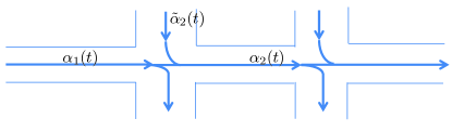
Figure 2: Two-light intersection

We consider a scenario in which a High-level (supervisory) controller has computed a traffic plan designed to manage congestion by balancing queue lengths, delays, and light-cycle times at the intersections. However, traffic bursts and other unpredictable events may cause traffic to deviate from its desirable behavior thereby leading to queue buildup. To mitigate these situations we regulate the intersections’ queue lengths by the duty ratios of the light cycles. We view this procedure as a mechanism for congestion avoidance which prevents the queue buildup at the second intersection from blocking traffic at the first intersection. Such acute congestion is assumed to be handled by a supervisory controller and is not discussed in this paper.

The regulation technique that we describe is comprised of tracking the queue lengths at the two intersections to given reference values which are assigned, for example, by the supervisory controller. The underlying traffic model consists of the fluid-queue system comprised of two queues in tandem, representing the respective queue buildup at the two intersections in the rightward direction shown in Figure 2. Let us denote the upstream queue by q1, and the downstream queue by q2. The inflow-rate process to q1 and the outflow process from it are $\{\alpha_{1}(t)\}$ and $\{\delta_{1}(t)\}$, respectively. A $\phi(t)$-fraction of the outflow process proceeds to the second queue, where it is multiplexed with the interfering process $\{\tilde{\alpha}_{2}(t)\}$ to form the inflow-rate process there, $\{\alpha_{2}(t)\}$, defined as $\alpha_{2}(t)=\phi(t)\delta_{1}(t)+\tilde{\alpha}_{2}(t)$.

Each of the queues has a constant light cycle of a given length, $C_{1}$ and $C_{2}$, comprised of red followed by green. The control variables of the system are the lengths of the red periods at the intersections, denoted by $\theta_{1}$ and $\theta_{2}$, respectively, and we define $\theta:=(\theta_{1},\theta_{2})^{\top}\in\mbox{$\mathbb{R}$}^{2}$ as the control vector. Naturally the length (duration) of the green periods are $C_{i}-\theta_{i}$, $i=1,2$. Note that some of the aforementioned rate processes depend on $\theta_{1}$ (like $\beta_{1}$, $\delta_{1}$, and $\alpha_{2}$), others depend on $\theta_{2}$ (like $\beta_{2}$), and $\alpha_{1}$ and $\tilde{\alpha}_{2}$ depend on neither $\theta_{1}$ nor $\theta_{2}$. To simplify the notation we will denote their dependence on $\theta$, as in $\beta_{1}(t,\theta)$, $\alpha_{2}(t,\theta)$, etc. The queue-lengths (occupancy) will be denoted by $x_{1}(t,\theta)$ and $x_{2}(t,\theta)$, respectively.

During red periods at queue $i$, $\beta_{i}(t,\theta)=0$. Upon a light switching from red to green, it is realistic to model the service rate as rising gradually rather than jumping to its highest rate. The definition of $\beta_{i}(t,\theta)$ reflects this in the following way: Let $kC_{i}$ be the starting time of the $kth$ cycle at queue $i$, whose red period and green periods are the time-intervals $[kC_{i},kC_{i}+\theta_{i})$ and $[kC_{i}+\theta_{i},kC_{i}+C_{i})$. Let $b_{i}(\tau)$ be a positive-valued, monotone-increasing random function of $\tau\geq 0$. We define $\beta_{i}(t,\theta_{i})=b_{i}(t-(kC_{i}+\theta_{i}))$ for every $t$ in the green period $[kC_{i}+\theta_{i},kC_{i}+C_{j})$. Summarizing the definition of $\beta_{i}(t,\theta_{i})$ in both red and green lights, we have,

$$\beta_{i}(t,\theta)=$$

$$\left\{\begin{array}[]{ll}0,&{\rm if}\ t\in[kC_{i},kC_{i}+\theta_{i})\\ b_{i}(t-kC_{i}-\theta_{i}),&{\rm if}\ t\in[kC_{i}+\theta_{i},kC_{i}+C_{i}).\par\end{array}\right.$$ (7)

Note that this definition of the service rate is quite general, and it includes the special case where $\beta_{i}(t,\theta)$ holds a constant value $\bar{\beta}_{i}$ during green periods.

Based on the fluid models of the queues, the buffer lengths $x_{i}(t,\theta)$ are related to the inflow and service rate processes by the following one-sided differential equation

$$\frac{dx_{i}}{dt^{+}}(t,\theta)=\left\{\begin{array}[]{ll}\alpha_{i}(t,\theta)-\beta_{i}(t,\theta),&{\rm if}\ x_{i}(t,\theta)>0\\ 0,&{\rm if}\ x_{i}(t,\theta)=0,\end{array}\right.$$ (8)

the outflow rate from the first queue, $\delta_{1}(t,\theta)$, is defined by

$$\delta_{1}(t,\theta)=\left\{\begin{array}[]{ll}\beta_{1}(t,\theta),&{\rm if}\ x_{1}(t,\theta)>0\\ \ \alpha_{1}(t),&{\rm otherwise},\end{array}\right.$$ (9)

and the input process to the second queue is defined as

$$\alpha_{2}(t,\theta)=\phi(t)\delta_{1}(t,\theta)+\tilde{\alpha}_{2}(t).$$ (10)

The problem that we consider is to regulate the queue lengths by adjusting $\theta$. Specifically, let us divide the time horizon into contiguous control cycles $\Gamma_{k}=[\gamma_{k-1},\gamma_{k})$, $k=1,2,\ldots$, and let $T_{k}:=\gamma_{k}-\gamma_{k-1}$ be the length of $\Gamma_{k}$. Defining $y_{i,k}:=\frac{1}{T_{k}}\int_{\Gamma_{k}}x_{i}(t,\theta)dt$ and $y_{k}:=(y_{1,k},y_{2,k})^{\top}$, the objective is to regulate $y_{k}$ to a given reference vector. The regulation will be carried out via repeated applications of Equations $(4)\rightarrow(2)\rightarrow(1)\rightarrow(3)$ (with $\theta$ replacing $u$) where the main challenge is to compute the gain $A_{k}$ defined in (4). This requires the IPA derivative of the plant function $G_{k}(\theta)$ defined as

$$G_{k}(\theta)=\displaystyle\frac{1}{T_{k}}\left[\begin{array}[]{c}\displaystyle\int_{\gamma_{k-1}}^{\gamma_{k}}x_{1}(t,\theta)dt\\ \displaystyle\int_{\gamma_{k-1}}^{\gamma_{k}}x_{2}(t,\theta)dt\end{array}\right],$$ (11)

whose computation is specified in the next subsection.

3.2 IPA Algorithm

For the sake of simplicity in the forthcoming discussion we will omit the dependence of $G_{k}(\theta)$, and other terms in (9), on $k$, and denote the generic $k$th control cycle by the interval $\Gamma=[0,T]$. By Eq. (4), it holds that

$$A\ =\left(\frac{\partial G}{\partial\theta}\right)^{-1}$$ (12)

where $G(\theta):=\big{(}G_{1}(\theta),G_{2}(\theta)\big{)}^{\top}$ is given by (9), and we next consider the computation of the IPA derivative $\frac{\partial G}{\partial\theta}$. Since both $\theta$ and $G(\theta)$ are two-dimensional, we will be concerned with the four partial derivatives, $\frac{\partial G_{i}}{\partial\theta_{j}}$, for $i,j=1,2.$

3.2.1 The case where $i=j$

By Eq. (11) we have, for $i=1,2$, that

$$G_{i}(\theta_{i})=\displaystyle\frac{1}{T}\displaystyle\int_{0}^{T}x_{i}(t,\theta_{i})dt,$$ (13)

and since $x_{i}(t,\theta_{i})$ is continuous in $t$,

$$\frac{\partial G_{i}}{\partial\theta_{i}}=\displaystyle\frac{1}{T}\displaystyle\int_{0}^{T}\frac{\partial x_{i}}{\partial\theta_{i}}(t,\theta_{i})dt.$$ (14)

Reference Wardi and Seatzu (2014), considering only a single-queue system, derived the following result for the term $\frac{\partial x_{i}}{\partial\theta_{i}}$. For $t$ lying in the interior of an empty period in queue $i$, $\frac{\partial x_{i}}{\partial\theta_{i}}(t,\theta_{i})=0$. On the other hand, for $t$ lying in the interior of a busy period in queue $i$, let $u_{t}$ be the starting time of the busy period containing $t$. Recall that $kC_{i}$ is the starting time of the $kth$ red period at queue $i$, and let $kC_{i}$, $k=\ell,\ldots,m$, be those points lying in the interval $[u_{t},t)$. Then

$$\frac{\partial x_{i}}{\partial\theta_{i}}(t,\theta_{i})=$$

$$\sum_{k=\ell}^{m}\beta_{i}((kC_{i})^{-},\theta_{i})+\beta_{i}(t,\theta_{i})-\beta_{i}(u_{t}(\theta_{i})^{+},\theta_{i}).$$ (15)

We point out that the rate-terms in (3.2.1) can be measured in real time by detecting the speed of passing vehicles. For details of these derivations please see Wardi and Seatzu (2014).

Eq. (3.2.1) is especially simple when $\beta_{i}(t,\theta)$ is equal to a given constant $\bar{\beta}_{i}>0$ during green-light periods at queue $i$. In that case it is readily seen that the first sum-term in the RHS of Eq. (3.2.1) is equal to $(m-\ell+1)\bar{\beta}_{i}$; $\beta_{i}(t,\theta_{i})\in\{0,\bar{\beta}_{i}\}$ depending on whether $t$ is in a red period or a green period, respectively; and similarly $\beta_{i}(u_{t}(\theta_{i})^{+},\theta_{i})\in\{0,\bar{\beta}_{i}\}$ depending on whether $t$ is in a red period or a green period, respectively. In this case the computation of $\frac{\partial G_{i}}{\partial\theta_{i}}$ is a matter of a simple counting process.

3.2.2 The case where $i\neq j$

It was mentioned earlier that we do not consider the case where the second queue blocks traffic at the first queue, and therefore $x_{1}(t,\theta)$ is a function of $\theta_{1}$ but not of $\theta_{2}$. Consequently, $\frac{\partial G_{1}}{\partial\theta_{2}}(\theta)=0$.

We next consider the partial derivative term $\frac{\partial x_{2}}{\partial\theta_{1}}(t,\theta)$. We will derive for it an event-based algorithm, where the events in question are light-switchings, jumps (instantaneous discontinuities) in traffic rates, and the beginning and end of busy periods at the queues. We say that two events are independent if neither event causes the other to occur at the same time. The following assumption is quite common in the literature on IPA of stochastic hybrid systems (e.g., Cassandras et al. (2002, 2010)).

Assumption 1

For a given control variable $\theta\in\mbox{$\mathbb{R}$}$, w.p.1, no two independent events occur at the same time.

We also implicitly assume that all of the derivative terms mentioned in the sequel exist w.p.1, and point out general and verifyable conditions guaranteeing this assumption (Cassandras et al. (2002, 2010)).

Before deriving the term $\frac{\partial x_{2}}{\partial\theta_{1}}(t,\theta)$ we mention four types of approximations that can be practical in implementations. These approximations will be used for computing the IPA derivatives but not for analysis of the traffic flows themselves which comprise the state of the “real” system. Therefore we expect the regulation scheme to work for a range of errors because of its aforementioned robustness. Some of these approximations are tested via simulation in Section 4 while others are the subject of current research. In the first approximation we assume that instantaneous traffic rates can be measured as, for instance, by speed detectors that are commonly used in traffic monitoring. Second, the fraction-term $\phi(t)$ is a mathematical construct that is well defined only for the fluid-flow model but not for the “real”, discrete system, and hence we replace it by a term $\phi\in[0,1]$ that can be computed, for example, by averaging traffic flows taken from real-time measurements. The derivative term $\frac{d\phi}{dt}(t)$ is neglected in the computation of the IPA derivative. Third, as mentioned earlier, we will test the decentralized version of the controller on traffic obtained from the correlated two-queue system. Fourth, we neglect in the forthcoming analysis the effects of delays in the control loop, which will be addressed in the future.

As for the term $\frac{\partial x_{2}}{\partial\theta_{1}}(t,\theta)$, consider separately the cases where $t$ lies in the interior of an empty period vs. a busy period in q2. If $t$ lies in the interior of an empty period in q2 then obviously

$$\frac{\partial x_{2}}{\partial\theta_{1}}(t,\theta)=0.$$ (16)

Consider next the case where $t$ lies in a busy period in q2, and denote by $p=p(\theta)$ the starting time of this busy period. Then

$$x_{2}(t)=\int_{p}^{t}(\alpha_{2}(\tau,\theta)-\beta_{2}(\tau,\theta))d\tau,$$ (17)

and therefore

$$\frac{\partial x_{2}}{\partial\theta_{1}}(t,\theta)=\frac{\partial}{\partial\theta_{1}}\Big{(}\int_{p}^{t}(\alpha_{2}(\tau,\theta)-\beta_{2}(\tau,\theta))d\tau\Big{)}.$$ (18)

Suppose first that $p$ lies in a q1-green period including the start of such a period, and that $t$ lies in a q1-green period as well. Let $[\eta_{i},\xi_{i})$, $i=1,\ldots,k$, denote the q1-red periods contained in the interval $[p,t)$ in increasing order, and define $\xi_{0}:=p$ and $\eta_{k+1}=t$, so that the intervals $[\xi_{i-1},\eta_{i})$, $i=1,\ldots,k+1$, are q1-green periods contained in the interval $[p,t]$.

Lemma 1

The following equation is in force,

$$\frac{\partial x_{2}}{\partial\theta_{1}}(t,\theta)$$

$$=-\big{(}\alpha_{2}(p^{+},\theta)-\beta_{2}(p^{+},\theta)\big{)}\frac{\partial p}{\partial\theta_{1}}$$

$$+\sum_{i=1}^{k}\big{(}\alpha_{2}(\xi_{i}^{-},\theta)-\alpha_{2}(\xi_{i}^{+},\theta)\big{)}$$

$$+\sum_{i=1}^{k+1}\frac{\partial}{\partial\theta_{1}}\int_{\xi_{i-1}^{+}}^{\eta_{i}^{-}}\big{(}\alpha_{2}(\tau,\theta)-\beta_{2}(\tau,\theta)\big{)}d\tau.$$ (19)

Moreover, the first term in the Right-Hand Side (RHS) of (17) is equal to 0 except in the following situation: the start of the q2-busy period at time $p$ is triggered by a jump up in $\beta_{1}(s,\theta)$ at the same time, $s=p$. In this case $\frac{\partial p}{\partial\theta_{1}}=1$, and the first term in the RHS of (17) is equal to $-\big{(}\alpha_{2}(p^{+},\theta)-\beta_{2}(p^{+},\theta)\big{)}$.

The proof can be found in the appendix. $\Box$

Remark 1

If a point $\tau\in[0,T]$ lies in the interior of a q1-red period then $\alpha_{2}(\tau,\theta)=\tilde{\alpha}_{2}(\tau,\theta_{2})$, which is independent of $\theta_{1}$. Therefore, if $q$ lies in the interior of a q1-red period then $\frac{\partial}{\partial\theta_{1}}\int_{q^{+}}^{\xi_{1}^{-}}\big{(}\alpha_{2}(\tau,\theta)-\beta_{2}(\tau,\theta)\big{)}d\tau=0$. In this case Equation (17) remains the same except that the sum in the last term of its RHS starts at $i=2$ instead of $i=1$. Likewise, if $t$ lies in the interior of a q1-red period then the last term of that sum is $i=k$ and not $i=k+1$.

The first two terms in the RHS of (17) involve flow rates which are assumed to be measurable. It remains to assess the third term in (17), which we next are set to do.

Consider the term

$$\frac{\partial}{\partial\theta_{1}}\int_{\xi_{i-1}^{+}}^{\eta_{i}^{-}}\big{(}\alpha_{2}(\tau,\theta)-\beta_{2}(\tau,\theta)\big{)}d\tau,$$ (20)

and recall that the interval $[\xi_{i-1},\eta_{i})$ is a green period in q1. Let us partition this interval into busy periods and empty periods in q1. Thus, define $[\tau_{b,1},\tau_{e,1})$ as the first q1-busy period in the interval $[\xi_{i-1},\eta_{i})$, $[\tau_{e,1},\tau_{b,2})$ is the following empty period, followed by the next busy period $[\tau_{b,2},\tau_{e,2})$, etc, and let $\tau_{e,m}$ denote the end-point of the last q1-busy period in the interval $[\xi_{i-1},\eta_{i}]$. Observe that if $\xi_{i-1}$ lies in a q1-busy period (or is the starting time of such a period) then $\tau_{b,1}=\xi_{i-1}$, and if $\xi_{i-1}$ lies in a q1-empty period then $\tau_{b,1}>\xi_{i-1}$. Likewise, if $\eta_{i}$ lies in a q1-busy period then $\tau_{e,m}=\eta_{i}$, and if $t$ lies in a q1-empty period then $\tau_{e,m}<\eta_{i}$.

Lemma 2

(I). If the interval $[\xi_{i-1},\eta_{i}]$ is contained in a single q1-busy period then

$$\frac{\partial}{\partial\theta_{1}}\int_{\xi_{i-1}^{+}}^{\eta_{i}^{-}}\big{(}\alpha_{2}(\tau,\theta)-\beta_{2}(\tau,\theta)\big{)}d\tau$$

$$=\phi\big{(}\beta_{1}(\xi_{i-1}^{+},\theta)-\beta_{1}(\eta_{1}^{-},\theta)\big{)}.$$ (21)

(II). Suppose that the interval $[\xi_{i-1},\eta_{i}]$ is not contained in a single q1-busy period. (i). If both $\xi_{i-1}$ and $\eta_{i}$ are included in two different q1-busy periods then

$$\frac{\partial}{\partial\theta_{1}}\int_{\xi_{i-1}^{+}}^{\eta_{i}^{-}}\big{(}\alpha_{2}(t,\theta)-\beta_{2}(t,\theta)\big{)}dt=$$

$$\phi\Big{(}\frac{\partial x_{1}}{\partial\theta_{1}}(\xi_{i-1})-\big{(}\alpha_{1}(\xi_{i-1})-\beta_{1}(\xi_{i-1}^{+}\big{)}\frac{\partial\xi_{i-1}}{\partial\theta_{1}}\Big{)}$$

$$+\phi\Big{(}\beta_{1}(\tau_{b,m}^{+})-\beta_{1}(\eta_{1}^{-})\Big{)}.$$ (22)

(ii). If $\xi_{i-1}$ is contained in the interior of a q1-empty period then the first additive term in the RHS os (20) is zero. (iii) If $\eta_{i}$ lies in a q1-empty period then the last additive term in the RHS of (20) is zero.

The proof can be found in the appendix. $\Box$

Remark 2

In (20), the term $\frac{\partial x_{1}}{\partial\theta_{1}}(\xi_{i-1})$ is assumed to be computable via (13) as applied to q1. It holds that $\frac{\partial\xi_{i-1}}{\partial\theta_{1}}=1$ for $i\geq 1$ (since $\xi_{i-1}=kC_{1}+\theta_{1}$), and $\frac{\partial\xi_{i-1}}{\partial\theta_{1}}=\frac{\partial p}{\partial\theta_{1}}$ for $i=1$ (since $\xi_{0}=p$).

The analysis leading to Lemma 1, Lemma 2, and the remarks that follow them imply that Algorithm 1, below, computes the IPA derivative $\frac{\partial x_{2}}{\partial\theta_{1}}(t,\theta)$ for $t$ lying in a q2-busy period. By (9), this will complete the computation of $\frac{\partial G_{2}}{\partial\theta_{1}}(\theta)$. The algorithm’s description focuses on a single q2-busy period, where we use the notation defined for the analysis in the earlier paragraphs. Thus, let $p$ be the starting time of the busy period and, in increasing order, let $\eta_{i}$ and $\xi_{i}$, respectively, $i=1,2,\ldots$, be the starting times of q1-red periods and green periods during the q1-busy period begun at time $p$. If $p$ lies in a q1-red period then we set $\eta_{1}=p$, while if $p$ lies in a q1-green period then we define $\xi_{0}=p$ and in this case $\eta_{1}>p$. In either case, $\xi_{1}>p$.

The algorithm computes, recursively, quantities $D_{i}$ at the times $\eta_{i}$, and quantities $E_{i}$ at times $\xi_{i}$. Furthermore, for every $t\in[\eta_{i},\xi_{i})$ (q1-red period) it sets $\frac{\partial x_{2}}{\partial\theta_{1}}(t,\theta)=D_{i}$, while for every $t\in[\xi_{i},\eta_{i+1})$ (q1-green period) it computes a function $g_{i}(t,\theta)$ (defined below) and then sets $\frac{\partial x_{2}}{\partial\theta_{1}}(t)=E_{i}+g_{i}(t)$. The algorithm has the following form.

Algorithm 1:

• At time $p$:
  If $p$ lies in a q1-red period: Set $\eta_{1}=p$, set $D_{1}=0$. For every $t\in[\eta_{1},\xi_{1})$, set $\frac{\partial x_{2}}{\partial\theta_{1}}(t,\theta)=0$.
  On the other hand, if $p$ lies in a q1-green period, set $\xi_{0}=p$, and set $E_{0}$ as follows: If the start of the busy period is triggered by a jump $\beta_{1}(\cdot)$, and $p$ lies in a q1-green and busy period including the start of such a period, set

  $$E_{0}=-\big{(}\phi\beta_{1}(p,\theta)-\beta_{2}(p,\theta)\big{)};$$ (23)

  otherwise, set $E_{0}=0$. Moreover, for every $t\in[\xi_{0},\eta_{1}]$, set

  $$\frac{\partial x_{2}}{\partial\theta_{1}}(t,\theta)=E_{0}+g_{0}(t),$$ (24)

  where $g_{0}(t)$ is defined below.

• At time $\eta_{i}$, $i=2,\ldots$:
  Set

  $$D_{i}=E_{i-1}+g_{i-1}(\eta_{i}),$$ (25)

  where the function $g_{i-1}(t)$ is specified later. Moreover, for every $t\in[\eta_{i},\xi_{i}]$, set

  $$\frac{\partial x_{2}}{\partial\theta_{1}}(t,\theta)=D_{i}.$$ (26)

  Note that the situation where $i=1$ corresponds to the case where $p$ lies in a q1-red period, which was discussed earlier.

• At time $\xi_{i}$, $i=1,2,\ldots$:
  Set

  $$E_{i}=D_{i}+\alpha_{2}(\xi_{i}^{-},\theta)-\alpha_{2}(\xi_{i}^{+},\theta).$$ (27)

  Moreover, for every $t\in[\xi_{i},\eta_{i+1}]$, define

  $$\frac{\partial x_{2}}{\partial\theta_{1}}(t,\theta)=E_{i}+g_{i}(t),$$ (28)

  where the function $g_{i}(t)$ is defined as follows.

• Definition of $g_{i}(t)$ for $t\in[\xi_{i},\eta_{i}]$, $i=0,1,\ldots$:
  If $t$ in the interior of a q1-empty period, set $g_{i}(t)=0$.
  On the other hand, if $t$ lies in a q1-busy period, we set $g_{i}(t)=g_{i,1}(t)+g_{i,2}(t)$, where the functions $g_{i,1}$ and $g_{i,2}$ are defined as follows. $g_{i,1}(t)$ depends on whether $\xi_{i}$ lies in the interior of a q1-empty period or in a q1-busy period. If $\xi_{i}$ lies in the interior of a q1-empty period then $g_{i,1}(t)=0$. On the other hand, if $\xi_{i}$ lies in a q1-busy period (including the start of such a period), then we define

  $$g_{i,1}(t)=\phi\Big{[}\frac{\partial x_{1}}{\partial\theta_{1}}(\xi_{i},\theta)-\big{(}\alpha_{1}(\xi_{i},\theta)-\beta_{1}(\xi_{i}^{+},\theta)\big{)}\frac{\partial\xi_{i}}{\partial\theta_{1}}\Big{]}.$$ (29)

  We point out that for every $i=1,2,\ldots$, the last term in (28) is $\frac{\partial\xi_{i}}{\partial\theta_{1}}=1$. In the special case where $\xi_{0}=p$, we have that $\frac{\partial\xi_{0}}{\partial\theta_{1}}=1$ as long as $p$ is a point in a green, busy period at q1, and the start of the q2-busy period begun at time $p$ is due to a jump up in $\beta_{1}$ at time $p$; in all other cases $\frac{\partial\xi_{0}}{\partial\theta_{1}}=0$.

  Consider next the function $g_{i,2}(t)$. If $t$ lies in the interior of a q1-empty period then $g_{i,2}(t)=0$. Likewise, if $\xi_{i}$ lies in a q1-busy period and $t$ lies in the same busy period, then $g_{i,2}(t)=0$. For the remaining case $t$ lies in a q1-busy period to which $\xi_{i}$ does not belong. In this case, define $\tau_{i,b}$ the starting time of the q1-busy period containing $t$. Then, $g_{i,2}(t)$ is defined as

  $$g_{i,2}(t)=\phi\big{(}\beta_{1}(\tau_{i,b}^{+},\theta)-\beta_{1}(t,\theta)\big{)}.$$ (30)

$\Box$

Remark 3

The algorithm looks quite complicated due to the need to track several types of events, but it is quite simple to code. Considerable simplification is likely to result from the likelihood that a single q1-green period is either contained in a single q1-busy period, or divided into a q1-busy period followed by a red period. It would be even simpler if the service rates at the queues have the form

$$\beta_{i}(t)=\left\{\begin{array}[]{ll}0,&{\rm if}\ t\ {\rm lies\ in\ a\ q1-red\ period}\\ \beta_{i,max},&{\rm if}\ t\ {\rm lies\ in\ a\ q1-green\ period}.\end{array}\right.$$ (31)

for given constants $\beta_{i,\max}>0$, since in this case $\beta_{i}(t,\theta)$ would be determined by whether $t$ lies in a red or green period. Even if this is not the case for “real” traffic, such a reasoning can be used in the IPA algorithm.

4 Simulation Examples

This section presents simulation examples for testing the effectiveness of the proposed regulation technique. The traffic-light cycles are is $C_{1}=C_{2}=1$, and each control cycle consists of 20 light cycles. The process $\{\alpha_{1}(t)\}$ consists of an off/on model where, in the off stage $\alpha_{1}(t)=0$, while for each on stage $\alpha_{1}(t)$ has a single drawn value uniformly distributed in an interval $[(1-\zeta)\bar{\alpha}_{1},(1+\zeta)\bar{\alpha}_{1}]$; we chose its mean to be $\bar{\alpha}_{1}=4.1$, and set $\zeta=0.3$. The durations of off periods and on periods are drawn from the uniform distributions on the intervals $[0,0.02]$ and $[0,0.063]$, respectively. The process $\{\tilde{\alpha}_{2}(t)\}$ is generated (drawn) in a similar way except that its mean value is $\bar{\alpha}_{2}=\bar{\alpha}_{1}/10=0.41$. This is motivated by the fact that the external arrival in the second queue is considered as noise that is not regulated by the traffic light. The main input flow in the second queue is assumed to come from the first queue, where we took $\phi=0.9$. The service-rate processes $\{\beta_{i}(t,\theta)\}$, satisfy Equation (29) with $\beta_{i,max}=5.0$, $i=1,2$. The set-point reference vector is $r=[0.1,\;0.1]^{\top}$, and the initial control variables were set to $\theta_{1}=\theta_{2}=0.8$.

Fig. 3 depicts the graphs of the obtained outputs $G_{1,k}(\theta)$ and $G_{2,k}(\theta)$ as functions of the counter $k=1,\ldots,50$, and we observe convergence in about 5 iterations. Fig. 4 provides the same information for $k=10,\ldots,50$ in order to highlight a variability of the output about the target values of 0.1, which is due to the randomness in the system. However, the respective means over the last 41 iterations, namely the quantities $\frac{1}{41}\sum_{k=10}^{50}G_{i,k}(\theta_{k})$, are $0.1001$ and $0.0986$ for $i=1$ and $i=2$, respectively.

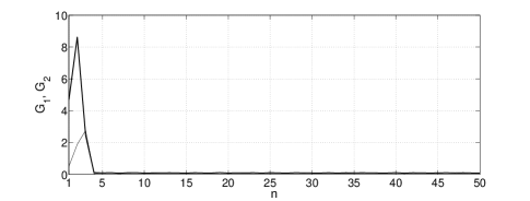
Figure 3: Evolution of $G_{1,k}$ (thick line) and $G_{2,k}$ (thin line) for $k=1\;\ldots,50$

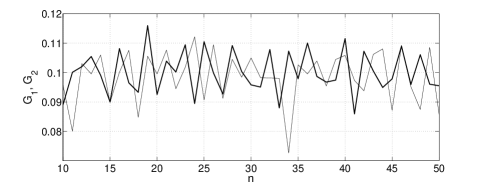
Figure 4: Evolution of $G_{1,k}$ (thick line) and $G_{2,k}$ (thin line) for $k=10\;\ldots,50$

Figure 5 shows plots of the control variables $\theta_{i,k}$, $k=1\ldots,50$, and we discern convergence to their respective values around $\theta_{1}\sim 0.3113$ and $\theta_{2}\sim 0.4129$. It is not surprising that the asymptotic value of $\theta_{2}$ is larger than that of $\theta_{1}$. The reason is that the input processes to the two queues have the same mean rate, but $\{\alpha_{2}(t,\theta)\}$ has less variance than $\{\alpha_{1}(t,\theta)\}$ due to the action of the first queue. Therefore, to obtain the same mean queue lengths the second queue would have a larger traffic intensity and hence smaller mean service rate, meaning that $\theta_{2}>\theta_{1}$.

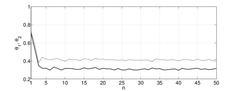
Figure 5: Evolution of $\theta_{1,k}$ (thick line) and $\theta_{2,k}$ (thin line) for $k=1\;\ldots,50$

A similar behavior, not shown here, was obtained with different values of the initial control variables as well as different values of the traffic parameters $\zeta$ and $\phi$.

	$mean|G_{1}(10:50)-r_{1}|$	$mean|G_{2}(10:50)-r_{2}|$	$\max G_{1}(1:50)$	$\max G_{2}(1:50)$
$\zeta=0.05$, centralized	$0.0843\cdot 10^{-3}$	$0.2575\cdot 10^{-3}$	$0.3507$	$4.7475$
decentralized	$0.0855\cdot 10^{-3}$	$0.0275\cdot 10^{-3}$	$0.3481$	$4.2749$
$\zeta=0.10$, centralized.	$0.0737\cdot 10^{-3}$	$0.1726\cdot 10^{-3}$	$0.7258$	$1.1770$
decentralized	$0.0637\cdot 10^{-3}$	$0.0415\cdot 10^{-3}$	$0.6633$	$1.9848$
$\zeta=0.15$, centralized.	$0.1505\cdot 10^{-3}$	$0.0753\cdot 10^{-3}$	$2.6368$	$1.9309$
decentralized	$0.2167\cdot 10^{-3}$	$0.0267\cdot 10^{-3}$	$2.5817$	$3.6931$
$\zeta=0.20$, centralized.	$0.1917\cdot 10^{-3}$	$0.4577\cdot 10^{-3}$	$4.9831$	$3.8481$
decentralized	$0.2094\cdot 10^{-3}$	$0.1458\cdot 10^{-3}$	$5.1314$	$7.7879$
$\zeta=0.25$, centralized	$0.2642\cdot 10^{-3}$	$0.6798\cdot 10^{-3}$	$7.2245$	$2.2578$
decentralized	$0.2731\cdot 10^{-3}$	$7.4621$	$7.4038$	$18.3908$
$\zeta=0.30$, centralized	$0.4617\cdot 10^{-3}$	$0.2643\cdot 10^{-3}$	$9.9984$	$3.0413$
decentralized	$0.4164\cdot 10^{-3}$	$8.4869$	$10.0046$	$20.9073$

Table 1: Comparison between centralized and decentralized regulation scheme.

We compared the joint, two-queue regulation scheme described in the last two sections with the decentralized control in which each queue computes its own gain (via (4)) without considering the effects of q1 on q2. The main difference is that in the second case the Jacobian $\frac{\partial G}{\partial\theta}$ is diagonal, and hence its computation is made much simpler: compare (13) to Algorithm 1. The comparison was made for various values of the input variance related to different choices of the traffic parameter $\zeta$. The results, shown in Table 1, comprise averages of 10 independent runs for each indicated value of $\zeta$, where in each run the first central moments of the output (columns 2 and 3) are computed over $k=10-50$ in order to avoid the effects of the early transients, while the maximum deviations (columns 4 and 5) are taken over $k=1-50$. It is evident that for lower variance $\zeta\leq 0,2$ the performances of the decentralized control is comparable to that of the centralized control. However, as the variance grows the errors associated with neglecting the derivative $\frac{\partial G_{2}}{\partial\theta_{1}}$ render the decentralized control unstable while the centralized controller works well.

5 conclusions

The main contribution of this paper is in a flow control technique in traffic-light intersections which aims at regulating queue lengths to given reference setpoints. The technique is based on multivariable integrators with adaptive gains computed using IPA. Numerical simulations are presented to corroborate the effectiveness of the proposed approach. A simpler, decentralized approach based on approximations designed to reduce the computing efforts is also considered, and its performance is shown (via simulations) to be similar to that of the multivariable integrators for a range of parameters.

6 Appendix

This section provides proofs to Lemma 1 and Lemma 2.

Proof of Lemma 1. By (16), Leibnitz rule, and the fact that $\eta_{i+1}=t$ is independent of $\theta_{1}$,

$$\frac{\partial x_{2}}{\partial\theta_{1}}(t,\theta)=-\big{(}\alpha_{2}(p^{+},\theta)-\beta_{2}(p^{+},\theta)\big{)}\frac{\partial p}{\partial\theta_{1}}$$

$$+\sum_{i=1}^{k}\Big{(}\alpha_{2}(\eta_{i}^{-},\theta)-\beta_{2}(\eta_{i}^{-},\theta)$$

$$-\big{(}\alpha_{2}(\eta_{i}^{+},\theta)-\beta_{2}(\eta_{i}^{+},\theta_{1})\big{)}\Big{)}\frac{\partial\eta_{i}}{\partial\theta_{1}}$$

$$+\sum_{i=1}^{k}\Big{(}\alpha_{2}(\xi_{i}^{-},\theta)-\beta_{2}(\xi_{i}^{-},\theta)$$

$$-\big{(}\alpha_{2}(\xi_{i}^{+},\theta)-\beta_{2}(\xi_{i}^{+},\theta)\big{)}\Big{)}\frac{\partial\xi_{i}}{\partial\theta_{1}}$$

$$+\sum_{i=1}^{k+1}\frac{\partial}{\partial\theta_{1}}\int_{\xi_{i-1}^{+}}^{\eta_{i}^{-}}\big{(}\alpha_{2}(\tau,\theta)-\beta_{2}(\tau,\theta)\big{)}d\tau$$

$$+\sum_{i=1}^{k}\frac{\partial}{\partial\theta_{1}}\int_{\eta_{i}^{+}}^{\xi_{i}^{-}}\big{(}\alpha_{2}(\tau,\theta)-\beta_{2}(\tau,\theta)\big{)}d\tau.$$ (32)

Light-switchings are events and hence, and by Assumption 1, the functions $\tilde{\alpha}_{2}(\tau)$ and $\beta_{2}(\tau,\theta)$ are continuous at $\tau=\eta_{i}$ and $\tau=\xi_{i}$, $i=1,\ldots,k$. Next, $\eta_{i}=kC_{1}$ and $\xi_{i}=kC_{1}+\theta_{1}$ for some $k=1,\ldots$, hence $\frac{\partial\eta_{i}}{\partial\theta_{1}}=0$, and $\frac{\partial\xi_{i}}{\partial\theta_{1}}=1$, rendering the first sum-term in the RHS of (30) to 0, and the last multiplicative term in the following sum-term to $\frac{\partial\xi_{i}}{\partial\theta_{1}}=1$. Furthermore, during q1-red periods $\alpha_{2}(\tau,\theta)-\beta_{2}(\tau,\theta)=\tilde{\alpha}_{2}(\tau)-\beta_{2}(\tau,\theta_{2})$ which is independent of $\theta_{1}$, and hence the last additive term in (30) is zero. In light of all of this, Equation (30) gives (17).

The last assertion of the lemma is obvious. $\Box$

Proof of Lemma 2. (I). Suppose that the interval $[\xi_{i-1},\eta_{i}]$ is contained in a q1-busy period. By definition, it is also contained in a q1-green period. Therefore, for every $\tau$ in this interval, $\alpha_{2}(\tau,\theta)=\phi\beta_{1}(\tau,\theta)+\tilde{\alpha}_{2}(\tau,\theta)$. Moreover, by definition and Assumption 1, the functions $\tilde{\alpha}_{2}(\tau)$ and $\beta_{2}(\tau,\theta_{2})$ and their jump times are independent of $\theta_{1}$. Consequently

$$\frac{\partial}{\partial\theta_{1}}\int_{\xi_{i-1}^{+}}^{\eta_{i}^{-}}\big{(}\alpha_{2}(\tau,\theta)-\beta_{2}(\tau,\theta)\big{)}d\tau=\phi\frac{\partial}{\partial\theta_{1}}\int_{\xi_{i-1}^{-}}^{\eta_{i}^{-}}\beta_{1}(\tau,\theta)d\tau.$$

But for every $\tau\in[\xi_{i-1},\eta_{i}]$ $\beta_{1}(\tau,\theta)=b_{1}(\tau-(kC_{1}+\theta_{1}))$ and hence $\frac{\partial\beta_{1}}{\partial\tau}(\tau,\theta_{1})=-\frac{\partial\beta_{1}}{\partial\theta_{1}}(\tau,\theta_{1})$, which implies (19).

(II). Consider case (i) where $\xi_{i}$ and $\eta_{i}$ lie in different q1-busy periods. The times $\tau_{b,j}$ and $\tau_{e,j}$ are event-epoch in q1 and hence, and by Assumption 1, the functions $\beta_{2}(\tau,\theta)$ and $\tilde{\alpha}_{2}(\tau)$ are continuous at these points. Next, $\eta_{i}$ is a switching time from green to red in q1, hence $\eta_{i}=kC_{1}$ for some $k=1,\ldots$, and therefore $\frac{\partial\eta_{i}}{\partial\theta_{1}}=0$. Furthermore, recall that the interval $[\xi_{i-1},\eta_{i})$ is contained in a q1-green period. Then for every $\tau\in(\tau_{b,j},\tau_{e,j})$, $j=1,\ldots,m$, $\alpha_{2}(\tau,\theta)=\phi\beta_{1}(\tau,\theta)+\tilde{\alpha}_{2}(\tau)$, and for every $\tau\in(\tau_{e,j},\tau_{b,j+1})$, $j=1,\ldots,m-1$, $\alpha_{2}(\tau,\theta)=\phi\alpha_{1}(\tau)+\tilde{\alpha}_{2}(\tau)$; this is independent of $\theta_{1}$ as is $\beta_{2}(\tau,\theta)$ and hence $\frac{\partial}{\partial\theta_{1}}\big{(}\alpha_{2}(\tau,\theta)-\beta_{2}(\tau,\theta)\big{)}=0$. Applying all of this with Leibnitz rule we obtain

$$\frac{\partial}{\partial\theta_{1}}\int_{\xi_{i-1}^{+}}^{\eta_{i}}\big{(}\alpha_{2}(\tau,\theta)-\beta_{2}(\tau,\theta)\big{)}d\tau$$

$$=\phi\Big{[}\sum_{j=2}^{m}\big{(}\alpha_{1}(\tau_{b,j}^{-})-\beta_{1}(\tau_{b,j}^{+},\theta)\big{)}\frac{\partial\tau_{b,j}}{\partial\theta_{1}}$$

$$+\sum_{j=1}^{m-1}\big{(}\beta_{1}(\tau_{e,j},\theta)-\alpha_{1}(\tau_{e,j})\big{)}\frac{\partial\tau_{e,j}}{\partial\theta_{1}}$$

$$+\sum_{j=1}^{m}\int_{\tau_{b,j}^{+}}^{\tau_{e,j}^{-}}\phi\beta_{1}(\tau,\theta)d\tau\Big{]}.$$ (33)

The first sum-term in the RHS of (31) is zero for the following reason: The point $\tau_{b,j}$ is the starting time of a q1-busy period. If it is triggered by a jump up in $\alpha_{1}(\tau)$ at $\tau=\tau_{b,j}$ then $\frac{\partial\tau_{b,j}}{\partial\theta_{1}}=0$ since $\alpha_{1}(\tau)$ is independent of $\theta_{1}$; it cannot be triggered by a jump down in $\beta_{1}(\tau,\theta)$ since this implies the end of a q1-green period, but we assume that the interval $[\xi_{i-1},\eta_{i})$ is contained in a q1-green period; and if it is due to a continuous rise of $\alpha_{1}(\tau)-\beta_{1}(\tau,\theta)$ from negative to positive then $\alpha_{1}(\tau_{b,j})-\beta_{1}(\tau_{b,j},\theta)=0$.

Next, for every $j=2,\ldots,m-1$, the interval $(\tau_{b,j},\tau_{e,j})$ comprises a q1-busy period, and hence $\int_{\tau_{b,j}}^{\tau_{e,j}}\big{(}\alpha_{1}(\tau)-\beta_{1}(\tau,\theta)\big{)}d\tau=0$. Taking derivatives with respect to $\theta_{1}$, we obtain,

$$-\frac{\partial}{\partial\theta_{1}}\int_{\tau_{b,j}^{+}}^{\tau_{e,j}^{-}}\beta_{1}(\tau,\theta)d\tau+\big{(}\alpha_{1}(\tau_{e,j})-\beta_{1}(\tau_{e,j},\theta)\big{)}\frac{\partial\tau_{e,j}}{\partial\theta_{1}}=0.$$ (34)

The case $j=1$ is different in that $\int_{\xi_{i-1}}^{\tau_{e,1}}\big{(}\alpha_{1}(\tau)-\beta_{1}(\tau,\theta)\big{)}d\tau=-x_{1}(\xi_{i-1},\theta)$, and similarly to the derivation of (32), we obtain,

$$\big{(}\alpha_{1}(\tau_{e,1})-\beta_{1}(\tau_{e,1},\theta)-\big{(}\alpha_{1}(\xi_{i-1}^{+})-\beta_{1}(\xi_{i-1}^{+},\theta)\big{)}\frac{\partial\xi_{i-1}}{\partial\theta_{1}}$$

$$=-\frac{\partial x_{1}}{\partial\theta_{1}}(\xi_{i-1},\theta).$$ (35)

By Equation (31) with the aid of (32) and (33), Equation (20) follows.

Finally, parts (II.ii) and (II.iii) of the lemma are obvious in light of the proof of part (II.i), since during a q1-empty period $x_{1}(\tau,\theta)=0$ and neither $\alpha_{2}(\tau,\theta)$ nor $\beta_{2}(\tau,\theta)$ depend on $\theta_{1}$. $\Box$

References

- Almoosa et al. (2012a) Almoosa, N., Song, W., Wardi, Y., and Yalamanchili, S. (2012a). A power capping controller for multicore processors. In Proc. American Control Conference. Montreal, Canada.
- Almoosa et al. (2012b) Almoosa, N., Song, W., Yalamanchili, S., and Wardi, Y. (2012b). Throughput regulation in multicore processors via ipa. In Proc. 51 IEEE Conference on Decision and Control. Maui, Hawaii.
- Cassandras and Lafortune (1999) Cassandras, C. and Lafortune, S. (1999). Introduction to Discrete Event Systems. Kluwer Academic Publishers, Boston, Massachusetts.
- Cassandras et al. (2002) Cassandras, C., Wardi, Y., Melamed, B., Sun, G., and Panayiotou, C. (2002). Perturbation analysis for on-line control and optimization of stochastic fluid models. IEEE Transactions on Automatic Control, 47(8), 1234–1248.
- Cassandras et al. (2010) Cassandras, C., Wardi, Y., Panayiotou, C., and Yao, C. (2010). Perturbation analysis and optimization of stochastic hybrid systems. European Journal of Control, 16, 642–664.
- Fleck and Cassandras (2014) Fleck, J. and Cassandras, C. (2014). Infinitesimal perturbation analysis for quasi-dynamic traffic light controllers. In Proc. 2014 Int. Workshop on Discrete Event Systems. Paris, France.
- Fu and Howell (2003) Fu, M. and Howell, W. (2003). Application of perturbation analysis to traffic light signal timing. In Proc. 42nd Conference on Decision and Control. Maui, Hawaii.
- Geng and Cassandras (2012) Geng, Y. and Cassandras, C. (2012). Traffic light control using infinitesimal perturbation analysis. In Proc. 51st IEEE Conf. Decision and Control. Maui, Hawaii.
- Geng and Cassandras (2013) Geng, Y. and Cassandras, C. (2013). Quasi-dynamic traffic light control for a single intersection. In Proc. 52nd IEEE Conf. Decision and Control. Florence, Italy.
- Geng and Cassandras (2015) Geng, Y. and Cassandras, C. (2015). Multi-intersection traffic light control with blocking. Discrete Event Dynamic Systems, to appear.
- Glasserman (1991) Glasserman, P. (1991). Gradient Estimation via Perturbation Analysis. Kluwer Academic Publishers, Boston, Massachusetts.
- Ho and Cao (1991) Ho, Y. and Cao, X. (1991). Perturbation Analysis of Discrete Event Dynamic Systems. Kluwer Academic Publishers, Boston, Massachusetts.
- Lancaster (1966) Lancaster, P. (1966). Error analysis for the Newton-Raphson method. Numerische Mathematik, 9, 55–68.
- Panayiotou et al. (2005) Panayiotou, C., Howell, W., and Fu, M. (2005). On-line traffic light control through gradient estimation using stochastic fluid models. In Proc. IFAC World Congress. Pragh, the Czech Republic.
- Wardi and Seatzu (2014) Wardi, Y., and Seatzu, C. (2014). Infinitesimal Perturbation Analysis of stochastic hybrid systems: application to congestion management in traffic-light intersections. In Proc. 53rd IEEE Conf. Decision and Control. Los Angeles, California.
- Wardi et al. (2015) Wardi, Y., Seatzu, C., Chen, X., and Yalamanchili, S. (2015). Performance regulation of stochastic discrete event dynamic systems using infinitesimal perturbation analysis. Nonlinear Analysis: Hybrid Systems, under review.
- Yao and Cassandras (2011) Yao, C. and Cassandras, C. (2011). Perturbation analysis and optimization of multiclass multiobjective stochastic flow models. Discrete Event Dynamic Systems, 21(2), 219–256.