Small- and Large-scale Characterization and Mixing Properties
in a Thermally Driven Thin Liquid Film

Abstract

Thin liquid films are nanoscopic elements of foams, emulsions and suspensions, and form a paradigm for nanochannel transport that eventually test the limits of hydrodynamic descriptions. Here we use classical dynamical systems characteristics to study the complex interplay of thermal convection, interface and gravitational forces which yields turbulent mixing and transport: Lyapunov exponents and entropies. We induce a stable two eddy convection in an extremely thin liquid film by applying a temperature gradient. Experimentally, we determine the small-scale dynamics using the motion and deformation of spots of equal size/equal color, we dubbed that technique “color imaging velocimetry”. The large-scale dynamics is captured by encoding the left/right motion of the liquid directed to the left or right of the separatrix between the two rolls. This way, we characterize chaos of course mixing in this peculiar fluid geometry of a thin, free-standing liquid film.

I Introduction

Chaotic or turbulent mixing is essential for many industrial processes, so a profound understanding is good for applications. However, despite the basic mechanisms for mixing in dynamical systems ottino1989kinematics ; doering1995applied are well understood, mixing characterization in experiments may be hard due to the real-world applications. Here, the restrictions are finite time, finite length and complex geometries. The system under consideration is an aqueous thin film, driven thermally. The film is almost two-dimensional and can show a thick phase (several $\mu m$) and a thin one ($\sim 10-50\,nm$), both immiscible due to the forces separating them, similar to bubbles (the thin phase) in a 3D liquid phase. The thinning speed of the film, i.e. the transition of the whole film to the thin phase depends primarily on the mixing of thin and thick phase. Without mixing, such a film typically undergoes thinning within several hours, with thermal driving, a flow is established that mixes the phases and leads to a thinning in a time of the order of seconds. Consequently, it is of high interest to understand this mixing and eventually quantify it. In the above mentioned article winkler2013exponentially the basic physics are explained. Here, we give a quantitative analysis of the mixing properties of the experiment in terms of Lyapunov exponents and entropies. We first discuss briefly the properties of thin liquid films, followed by an explanation of our approach to the characterization of mixing for this highly sophisticated system.

Thin film dynamics is governed by gravitational, capillary and interfacial forces, where the latter are specified in the disjoining pressure. Combining long- and short-range molecular forces: electrostatic, van der Waals (vdW), and steric forces derjaguin1989theory ; oron1997long , the disjoining pressure depends strongly on the distance between the interacting surfaces. Whereas films on substrates are established in industry and research reiter1998artistic , freestanding thin liquid films still provide a challenge in experiments and theory alike. Consequently, the study of foam films is central to current scientific activities, e.g. kellay2011turbulence ; yunker2011suppression ; davey2010enantiomer ; Prudhomme-Khan-96 ; exerowa1998foam ; vermant2011fluid . We contribute by presenting a way to quantify mixing of vertically oriented, freestanding, thermally forced, nonequilibrium foam films.

As a result of the aforementioned force balance two stable equilibria may occur, depending on the chemical composition of bulk solution and chosen surface active agents (surfactants): Common Black Films (CBF) with a thickness of more than 10 nm are formed when electrostatic interactions balance the dominant van der Waals force, and, of course, gravity and capillarity derjaguin1989theory ; Verwey-Overbeek-48 ; Newton Black Films (NBF) are stable with a thickness of less than 10 nm, due to repulsive short range steric forces jones1966stability ; israelachvili1991intermolecular . In this study we will focus on films in their transient phase before reaching equilibrium with a typical thickness in the range of $0.1-1\,\mu m$. The effect of additional forces has been studied by a several authors, mostly for micrometer-thick systems zhang2005velocity ; seychelles2008thermal .

Quantifying the degree of complexity of an evolving system is an ubiquitous problem in natural science badiicomplexity . We will focus on two ways of measuring dynamical complexity: the metric or Kolmogorov-Sinai entropy $h_{KS}$, which measures the rate of information production as a fluid particle evolves along a pathline, and the Lyapunov exponents (LEs), which give the rates at which nearby fluid paths diverge. The principle concept of the KS-entropy is very natural, as the information contained in the time evolution is a characteristics of the underlying dynamics, cf. Brudno’s theorem batterman1996chaos .

From data, one can obtain an estimate by studying the symbolic dynamics acquired by assigning different symbols to different “cells” of a finite partition of the phase space. The probability distribution of realized sequences (words) is a signature dynamical evolution. The average information gain is obtained by comparing sequences of length m and m+1, in the limit of large m: letting the length of the words, m, to infinity and the partition diameter to zero, one obtains the KS-entropy, which is often used as a “measure of complexity” of a system.

Lyapunov exponents $\lambda$ characterize the exponential divergence of nearby trajectories, typical for chaotic systems ott2002chaos ; kantz2004nonlinear . One can alternatively state that LEs characterize the sensitivity of a system to initial conditions $X_{i}$. They are related to the KS-entropy $h_{KS}$ by the Pesin formula:

$$h=\sum_{i=1}^{n}\lambda_{i}>h_{KS}\;.$$ (1)

Positive Lyapunov exponents indicate that solutions diverge exponentially on average, negative ones indicate convergence. They are computed from time series using embedding techniques kantz2004nonlinear , in our case, we can use the spatial information directly and use instead stretching and folding of a fluid area to estimate the local dynamical characteristics directly from the experiment.

II The Experiment

In this section, we describe in detail the experiment, the flow structure which is crucial for the analysis. Then, we explain the data analysis we applied, first for the LEs, then for the entropies. In principle, we follow complementary approaches: the LEs are computed from microscopic information, whereas the entropies are determined from the large-scale circulation. Ideally, both quantities should coincide, to be tested by Pesin’s formula. We will show the results below.

II.1 Setup

The experimental setup consists of a vertical rectangular aluminium frame with rounded corners, 45×20 mm, enclosed by an atmosphere-preserving cell with a glass window for video recording, cf. Fig. 1. Thermal forcing is effected by inserting a cooled copper needle (radius 1 mm) at the film center ($T=-169$ ^∘C), the needle enters the cell through a fitting hole. Ambient temperature was constant at 20 ^∘C, the corresponding Rayleigh number $Ra\sim 10^{6}$, such that the flow is clearly turbulent. Please note that for very thin films it is not clear how viscosity changes with the film thickness, since surface forces may matter. We are not aware of any investigations in that direction, and will not discuss this further. The given number denotes an order of magnitude, such that only dramatic changes in viscosity are relevant, e.g. if the film has a transition to thin black film and changes structure, too. The temperature across the film (z-direction, cf. Fig. 1) is approximately constant, and the Marangoni number $Ma\simeq 0$ . The solution from which the liquid film was drawn consists of the surfactant n-dodecyl-$\beta$-maltoside ($\beta\mathrm{-}C_{12}G_{2}$), prepared with filtered deionized water and stabilized with 25 $\%_{\rm vol}$ glycerin stoeckle2010dynamics . The thin liquid film is illuminated with a diffuse broad spectrum light source and its reflection is captured by a high speed camera. Our vertically oriented foam film is produced initially thick (500 – 5000 nm) by pulling it with a glass rod from the reservoir. Quickly, a wedge-like profile develops with BF in a small region, with a sharp horizontal boundary towards the thick film below, cf. Fig. 2.

The interference of incident and reflected light yields a striped pattern, which can be used to infer the film thickness. Each color cycle (red $\rightarrow$ blue) corresponds to multiples $n$ of the smallest negative interference condition $(2\cdot n+1)\lambda\eta=4h\cos\Theta$, where the refraction index, $\eta$, is assumed to be temperature-independent; $\Theta$ is the angle of incidence atkins2010investigating . The velocity is measured by color imaging velocimetry (CIV) winkler2013mixing with $u\sim 0.02\,\nicefrac{\mathrm{m}}{\mathrm{s}}$.

For ideal 2D flows -turbulent or not- surface forces are neglected. This is reasonable for thick films. In our case, a full description involves all occurring forces winkler2013exponentially . For the Rayleigh number we are working with, $Ra\sim 10^{6}$, other forces can be neglected to first order. Surfactants stabilize the film, which is confirmed by our experiment, even if the film is heated (giving rise to thermal fluctuations) and if the entire film is black, and of the thickness of a few nanometers (giving rise to sensitivity to other molecular forces). The turbulence generated by the cold needle is observable with the naked eye, a snapshot shown in Fig. 2.

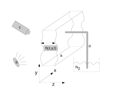
Figure 1: Setup of the experiment. (a) schematic sketch of the free-standing thin film, (b) light source, (c) camera, (d) cooling rod with liquid nitrogen reservoir.

II.2 Flow Description

This publication presents experimental work and subsequent data analysis, thus we do not discuss the equations of motion of the film, but refer to recent work and reviews for the suiting equations in our situation Kruesemann-2012 ; oron1997long ; erneux1993nonlinear . However, we now discuss the observations in order to give the reader an impression about the flow we consider in terms of dynamical systems properties.

We use a point thermal force to drive our system, such that we have two rolls, one on each side of the cooling rod, cf. Fig. 2. The cold rod drives a stable two-eddy convection with a jet of fluid in the center as the driving mechanism and separation at the same time. The deflection of the jet at the lower frame border is sequential and non-deterministic. For the analysis of the large-scale flow, the alternation between the left and the right eddy/vortex was visually tracked, recorded during a long time interval and converted into a binary time series as detailed in section II.3. Further information on this technique is available in our previous works winkler2013exponentially ; winkler2011droplet ; winkler2013mixing .

In an abstract way, our flow can be described by geometry (boundary conditions) and four fixed points: the flow is bounded by the enclosing rectangle, which in the upper region is given by the black film region. Boundary conditions are complicated, in a first step they are assumed no-slip. Then, we have the centers of the convection rolls, which are elliptic fixed points There are two hyperbolic points at the bottom and directly below the lowest part of the ice surrounding the cooling needle and a separatrix running top-down (cf. Fig. 3), whose connection form a separatrix. This description holds on short time scales, for long times, we must consider that the whole system is in a transient state which, however evolves on much larger time scales, such that our considerations are reasonable. A look at corresponding video material will clarify this characterization.

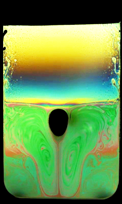
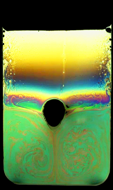
Figure 2: Snapshot of a turbulent convecting thin film. An image of the non-moving film has been subtracted, the frame and frozen center region including the cooling tip are not shown. On the sides, the typical meandering of rising thin/sinking thick film is observed. On the top, a layer of black film has formed which is transported downwards. Thickness can be read from the colors. Left: The convection is not yet fully developed, such that “corner” vortices are observed; they disappear after transients. Right: Turbulent convection has fully developed and thin film is transported and mixed quickly by the convection.

We want to characterize the flow, based on measurements. Key characteristics for mixing and flow in general are stretching or folding of the liquid filaments. We consider respective orbits of fluid elements advected by the two convection rolls, which are stably positioned below the cooling rod. One key question regards the mixing inside the rolls, the other one mixing between the rolls. In contrast to other systems, as e.g. the blinking vortex ottino1989kinematics , the vortices are maintained and mixing happens across the separatrix due to small differences in the middle downward flow. Conceptually, we can use the basic ideas of twist maps, as one common example for reduce dynamical systems showing mixing. I.e. we study the left-right transport, i.e. the mixing between the two rolls.

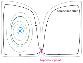
Figure 3: Orbit schematic for the presented experiment (only the right half of the convection zone is shown in detail). The light gray outer line represents the shape of the two convection zones in the experiment. The gray traces represent orbits moving away or towards the center of convection. The elliptic orbits are marked with a light blue circle around the stationary elliptic point (blue cross) in the center of the convection zones. Green marks the limit between converging and diverging orbits.

Below, in Sec.II.3, we explain how typical stretching rates are extracted from the experiment, as described in more detail in winkler2013mixing . We recall the procedure briefly here, in order to be complete. Then, we step to an analysis in terms of symbolic dynamics in that we analyze the series of liquid transported left and right, i.e., we reduce flow to the fluid exchange between the two rolls. This way we have a local measure by the stretching and a more global one by the transport across the separatrix.

II.3 Data Analysis

The captured video data is post-processed to enhance colors and contrast. To analyze the behaviour of domains of the same thickness the video is converted into a binary image where white corresponds to a single color respectively thickness. As the spectrum repeats continually this technique is only valid if the overall thickness deviation is smaller than a full period of the smallest wavelength. Subsequently in each frame all clusters of the same thickness are numbered and consecutively linked through the following frames (Fig. 4). This enables us to track the volume, velocity, deformation rate and angular velocity of the moving fluid. For each cluster the velocity is calculated using the shift of its center of mass per frame. The deformation rate is calculated by determining the change of the scale of the principal components per frame. Similarly the angular velocity is given by the rotation of the principal component. Averaging over all frames then delivers the spatial characteristics of the flow field generated by the cooling tip. The cluster finding algorithm is operating with a linear backwards memory of variable depth. However for now a tracking of one frame backwards is sufficient to maintain connectivity of each cluster through all frames. The memory needs to be limited as merging or dividing clusters would be considered connected, thereby distorting the velocity and deformation rate.

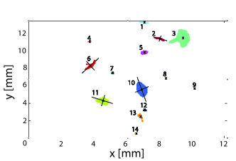
Figure 4: example of the cluster identification for one frame, including center of mass and selected principle components (not to scale).

The intermittency of the mixing film is captured by the probability $P(\Delta x,\Delta t)$: we calculate the distance $\Delta x$ for fixed $\Delta t$ (on logarithmic scale). The result is plotted in Fig. 5. We observe basically ballistic transport for small $\Delta t$, as could be expected because the more chaotic small scales are not resolved, and the large scale transitions are not found by our cluster analysis.

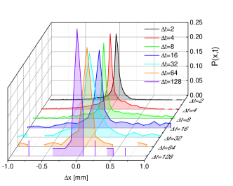
Figure 5: Probability $P(\Delta x,\Delta t)$ for different time scales $\Delta t$(unit: frames, framerate: 100 frames per second). The transport is ballistic over one decade. Larger times are not shown due to the insufficient number of data.

In the generated velocity field (Fig. 6) the fluid is stretched in regions of high velocity and compressed when it enters areas of lower velocity. Due to the shear which is present between layers of different velocity folding happens. These two processes are the main aspects of mixing in a two dimensional fluid. Diffusion processes can be neglected as the Reynolds number is of the order of $10^{3}$.

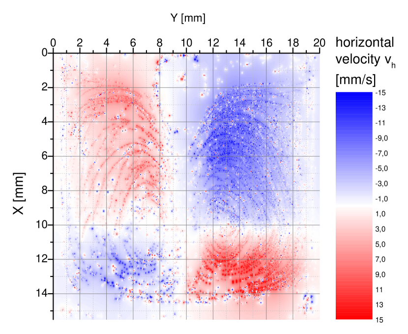
(a) horizontal velocity

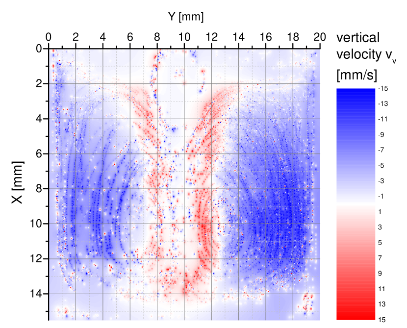
(b) vertical velocity

Figure 6: averaged velocity field of the forced advection. The cooling rod is positioned at approximately $p_{rod}(x,y)=[2\,mm,10\,mm].$

The overall mixing can be characterized within each vortex as an averaging of the stretching rate over the vortex area. The global mixing between the vortices is characterized by the probability of a fluid element to cross the separatrix. This procedure can be seen in the view of effective diffusion, because the averaged turbulent velocity field is a kind of random walker with possibly anomalous and space dependent transition rates, which when averaged yield the diffusion coefficient. The transition from one cell to the other is the minimal setup, as discussed in abel2000exit .

We use a naive approach to analyze our film: take a spot of material of size $\Delta x$, compute its time derivative approximatively from the time evolution as finite difference and use then averaging to determine the macroscopic properties. This is in contrast to studies with particles, where the velocity of relative dispersion is calculated, and only possible because we have already a field at hand. From the clusters of the same thickness, we obtain the eigenvalues $e_{1,2}^{i}$ along the principal axes; they correspond directly to the size of the spot numbered $i$. Averaging the $e^{i}$ over time and filtering yields an estimate for the fields $e_{1,2}(x,y)$. Now we compare that with the definition of the diffusion coefficient:

$$D=\lim_{\Delta t\to 0}\frac{\left<(x(t+\Delta t)-x(t)^{2}\right>}{\Delta t}\;.$$

In our situation the limit cannot be reached, due to sampling and consequently we should use methods like the FSLE Aurell-Boffetta-Crisanti-Paladin-Vulpiani-96 , which are ongoing work. Here we show the results for the finite-size spots with $\Delta t=\Delta_{s}$ fixed to the minimal sampling time. We make of course an error in mixing different spot sizes, which we counteract by choosing homogeneous spots of similar size.

The space–dependent diffusion is then estimated by

$$D_{est}={\frac{\left<x(t+\Delta_{s}t)-x(t)^{2}\right>}{\Delta_{s}}}$$

where averaging over many times ($\sim 10^{6}$) is performed. Of course this is a very rough approach, but we will see that in a certain time range we obtain reasonable results, and can compare this with the enhancement of thinning. This is, however not the full story: for mixing it can be desirable to have faster than normal diffusion, the characterization of a real process involves finite intervals $\Delta t$, $\Delta x$, and the degree of anomaly is given by the scaling $\Delta t\sim\Delta x^{\alpha}$, with $\alpha=2$ for normal diffusion. since we prescribe $\Delta t$ and determine $\Delta x$ accordingly, the full statistical characterization is given by the probability function $P(\Delta x,\Delta t)$, cf. Fig. 5.

So, we characterize mixing within the two rolls by an effective diffusion approach and the mixing between the two rolls by statistics of the crossings of the separatrix in the middle of the setup.

The fluid itself offers no contrast to track the motion of filaments. However, the above described reflection imaging transforms the relative thickness difference of convected filaments into a thickness map whose evolution can be followed and analyzed. Compared to other techniques like seeding beads or injecting ink, which are unpractical due to the resulting perturbation of the thin liquid layer, the thickness tracking is non invasive and precise. A drawback (not important here) is that only a relative instead of an absolute thickness map is available and fine layering of filaments is subject to diffusion, thus limiting the resolution.

In this study we investigate as well on the center stream in between the two stable vortices which is deflected either to the right or to the left at the bottom of the frame. At the cooling rod fluid from both vortices is formed into a center stream. As the convection is bound by the frame the center jet is deflected sequentially to the left or to the right at the bottom hyperbolic point. This gives a relative measure of the amount of fluid mixed m,acroscopically between the left and right eddy. The binary series of transports can then be used to estimate the efficiency of this mechanism by calculating the entropy and stochastic properties.

III Methods and Results

In this section, we present methods and results based on the data obtained as described above. A first subsection treats Lyapunov exponents, estimated by the stretching and folding of small fluid elements. In this sense we only find finite-size values, which characterize the small-scale properties of the flow (and not the infinitesimal ones, as one would need for the true Lyapunov-exponents). Within that subsection we briefly recall and comment on the relation of measures from mixing theory and dynamical systems. In the second subsection results on the estimation of entropies are shown. We estimate the characteristic entropies by the symbolic dynamics approach abel2000exit ; kantz2004nonlinear forming words of a certain length, compute their frequencies as estimators of the probabilities, and eventually obtain an estimate for the entropy production with increasing word length. At the end of this section we compare both measures using known relations.

III.1 Lyapunov Exponents

In dynamical systems theory, Lyapunov exponents (LE) are key quantities for the characterization of systems. an equivalent is the efficiency in mixing theory for fluids. Essentially, in a fluid, the stretch of a fluid filament is important, analogous to the stretching of a phase space element in a dynamical system. In our case, both quantities are identical. Furthermore, the mixing efficiency is nothing but a normalized version of the Lyapunov exponent for an ergodic system, since time and ensemble average need to coincide for the equivalence to hold.

In the following we describe how to estimate mixing efficiency and LEs $\lambda$ starting from the stretch $s$ of a fluid filament along its trajectory, where

$$s=\lim_{\Delta x_{0}\to 0}\frac{\Delta x_{t}}{\Delta x_{0}}\;$$ (2)

for the fluid velocity measured in the Eulerian (i.e. laboratory) frame. $\Delta x_{0}$ denotes the initial separation of two “fluid points“ at time $t=0$, and $\Delta x_{t}$ the corresponding separation at time $t$. To satisfy the limit towards elements $\Delta x_{0}$ of infinitesimal length, the cluster data was filtered to contain only the smallest clusters available. The local stretching rate $\frac{ds}{dt}$ (cf. Fig.7) is measured in a moving reference system (Lagrangian), therefore the velocity of the separating edges of a fluid filament are observed.

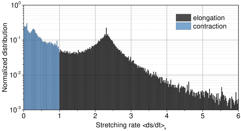
Figure 7: Semi-logarithmic plot of the spatially-averaged stretching distribution. Larger and smaller unity is marked differently for better visibility. The main difference lies in the behaviour for contracting values, which can be zero, i.e. the spot observed vanishes. This is reminiscent of our data analysis, explained above and is not expected for a perfect measurement.

The Lyapunov exponents $\lambda$ describe the typical property of chaotic systems, in particular 2D systems with hyperbolic points: the trajectories of two nearby points diverge exponentially. We can relate that to fluid motion, for details cf. e.g. ott2002chaos ; tel2006chaotic . The exponential divergence for infinitesimally small times is expressed as $\Delta x_{t}\sim{\Delta x_{0}}e^{\lambda t}\;.$ The local Lyapunov exponent is then given as the long time average of the logarithmic stretching rate (cf. Fig. 8):

$$\epsilon_{s}=\frac{D\ln s}{Dt}\;\rightarrow\;\lambda_{l}=\lim_{t\rightarrow\infty}\frac{1}{t}\int\limits_{0}^{t}\epsilon_{s}\mbox{d}t^{\prime}\;,$$ (3)

where we recognize the difference to the stretch (eq.2) in averaging the logarithm or the ratio of the lengths directly. For ergodic systems, time and (phase) space average are identical and we can compute alternatively

$$\left<\lambda\right>_{x,t}=\left<\lim_{\Delta x_{0}\to 0}\lambda_{l}\right>_{x}\;.$$ (4)

with the notation $\left<\,\right>_{x}$ for the space average. We can compute the two Lyapunov exponents from the contraction (-) and elongation (+) of the tracked fluid filaments and obtain as an estimate on the overall mixing properties of the flow:

$$\left<\lambda_{-}\right>_{x,t}=-1.43\;,\left<\lambda_{+}\right>_{x,t}=0.92\;.$$ (5)

If the flow is conservative $\||\lambda_{-}/\lambda_{+}=1\||$, here we find a contraction considerably smaller than $-1/0.92\simeq-1.087$. It is explained by the fact that we do not only measure the stretch, but in addition the general volume loss of a spot of a certain color due to film thinning and diffusion of the thickness map, as explained above, cf. Fig.4; this contributes to the negative LE.

The distribution of the positive and negative LE are quite different. This is explained by the dynamics: elongation -positive LE- takes place mainly in the rapid flow region between the two fixed points (the separatrix). This leads to a very pointed distribution with faster than exponential decay, cf. Fig. 8, black marked part. In contrast to this contraction happens over the whole region of the film with quite different and much slower dynamics. Additionally, the contraction rate data has a lower signal to noise ratio compared to the elongation rate, as the absolute values are smaller and closer to the resolution limit of the setup.

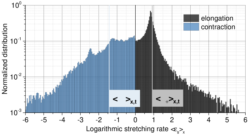
Figure 8: Distribution of the stretching rate $\epsilon_{s}$. The average over time gives the Lyapunov exponents $\left<\lambda_{-}\right>_{x,t}=-1.43\;,\left<\lambda_{+}\right>_{x,t}=0.92$, indicated by the vertical lines. Clearly, the distribution of negative and positive LE ist different.

Before stepping to the estimation of the entropy we want to describe the connection between LE and mixing efficiency, both quantities are closely related:

$$\left<E_{s}\right>=\frac{1}{t}\int\limits_{0}^{t}\frac{\epsilon_{s}}{\sqrt{\vec{D}:\vec{D}}}\mbox{d}t^{\prime}$$ (6)

We see that the difference lies in the nhe normalization. It involves the symmetric part of the velocity gradient $\vec{D}=\frac{1}{2}\left[\nabla\vec{v}+(\nabla\vec{v})^{T}\right]$ (equivalent to the stretching tensor), where $\vec{D}:\vec{D}$ needs to be constant over the pathlines, for this expression to be valid. It is used as a normalization to obtain a stretching efficiency smaller or equal to one. Using this normalization, one can demonstrate ottino1989kinematics that the upper bound of the efficiency for two-dimensional flows is $E_{s,max}=\sqrt{2}/2=0.707$ ottino1989kinematics . Since the stretching tensor is not readily available from the cluster data and is only used as a normalization in Eq. 6 it was not used here and we refer to the unnormalized Lyapunov exponents.

III.2 Entropy

Similar to the Lyapunov exponent the entropy production of a dynamical system is a measure of its chaoticity. Here we compute the Kolmogorov-Sinai entropy $h_{KS}$for the center jet deflection and compare it to $\left<\lambda_{-/+}\right>_{x,t}$ which we obtain from the stretching rates of the fluid filaments. The topological entropy $h$ is the upper limit for average Lyapunov exponent: $h\geq\left<\lambda\right>$ tel2006chaotic and the Pesin formula equates the topological entropy with the sum of all positive Lyapunov exponents: $h=\sum_{i=1}^{n}\lambda_{+,i}>h_{KS}$, and sets the limit for $h_{KS}$ ruelle1989chaotic . More precisely the relation between the topological entropy $h$ and $h_{KS}$ is given via the Variational Principle: $h(T)=\mbox{sup}\left(h(\mu)_{KS}:\mu\in\mathcal{P}_{T}(X)\right)$, where $\mu$ ranges over all T-invariant Borel probability measures on X. Thus $h$ is an upper limit for the KS-entropy. A direct relation between Lyapunov exponents and entropy is available via the information dimension

$$D_{I}=h(\mu)\left(\frac{1}{\left<\lambda_{+}\right>_{x,t}}+\frac{1}{|\left<\lambda_{-}\right>_{x,t}|}\right)$$ (7)

of an ergodic invariant measure $\mu$ of a smooth invertible map with Lyapunov exponents $\left<\lambda_{+}\right>_{x,t}>0>\left<\lambda_{-}\right>_{x,t}$ young1982dimension ; ott2002chaos . $\left<\lambda_{-/+}\right>_{x,t}$: Lyapunov exponents calculated from stretching (+) and contraction (-) rates.

Comparing Eq 7 to the Kaplan-Yorke conjecture frederickson1983liapunov : $D_{L}=1+\left<\lambda_{+}\right>_{x,t}/|\left<\lambda_{-}\right>_{x,t}|$ , with Lyapunov dimension $D_{L}$, suggests that $h(\mu)=\left<\lambda_{+}\right>_{x,t}$ in the case of the natural measure of a 2D smooth invertible map.

Let us now compute the values for the entropy to the degree our data allow with respect to length of the time series and accuracy. First, we need to define a kind of “alphabet” to identify words. Our procedure follows essentially abel2000exit and for more details we refer to that publication. The jet is deflected either into the left or into the right vortex at the bottom of the frame. We analyze the deflection pattern to check for deterministic components, which would lower the mixing efficiency of this fluid transport.

The sequence of left (treated as 0) and right (treated as 1) transports is a binary time series from which one can associate a word of length $n$, out of a finite alphabet: $W_{k}^{n}=(S_{k},S_{k+1},...,S_{k+n-1})$. The block entropies $H_{n}$ are then calculated from the word probability distributions $P(W^{n})$:

$$H_{n}=-\sum_{W^{n}}P(W^{n})\ln\,P(W^{n})$$ (8)

where $W^{n}$ represents the set of all possible words of length n. The entropy per unit time is defined as:

$$\begin{split}h_{n}&=H_{n+1}-H_{n}\\ h_{KS}&=\lim\limits_{n\rightarrow\infty}{h_{n}}\end{split}$$ (9)

In the presented case the practical limit of $h_{KS}$ is given by the finite series of events thus truncating the number of possible words and the possible entropy gain by increasing the word length. $h_{n}$ can be interpreted as the rate of information production, which for a finite signal decreases when the combined length of all possible words $W^{n}$ becomes larger than the signal itself: $\sum_{W^{n}}n>l_{S}$. The mixing efficiency is maximal when the jet deflection is equally distributed for left and right. Therefore, we use a set of equal left/right probability as a benchmark for the measurement data . As expected, the entropy $h_{n}$ remains constant with increasing word length until the finite size limit of the data set is reached, and longer sets hit this limit at higher word lengths, cf. Fig. 9(a).

The entropy $h_{n}$ of the different distributions below this limit is identical, in particular for the data with the same length as the measurement set. Therefore, the deviation in $h_{n}$ of the measurement data when compared to the equally dstributed data sets cannot simply be omitted as a finite size effect. $h_{n}$ of the measurement data is approximately 15-20% below the possible maximum given by the random sequences, which indicates a non-uniform process or deterministic behaviour, cf. Fig. 9(b).

One might assume that the sequence is tilted towards one side and that this preference causes the flow pattern to be more predictive. To check for this property we compared the data set to skewed random distributions which have a lower entropy production due to the higher predictability of the signal. In Fig. 10 random sets with an uneven distribution up to a probability of $P=0.9$ for one direction of the flow are compared. The entropy production of a $77/23$-skewed distribution is comparable to the measurement data. In this case the deflection of the center jet would be directed towards one side approximately 8 out of 10 times. However, the distribution of left and right transports in the measurement data is even which shows that the deterministic components of the signal is not due to a simple asymmetry in the experimental setup.

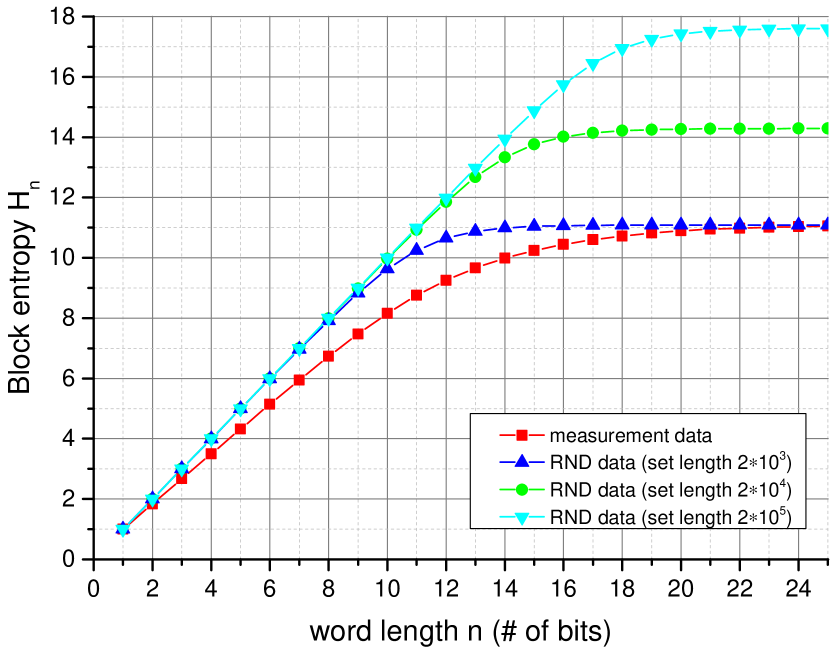
(a) Block entropy $H_{n}$

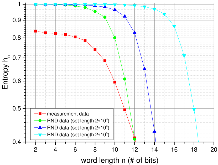
(b) Entropy $h_{n}$

Figure 9: Block entropy $H_{n}$ and entropy $h_{n}$ with increasing word length of the measurement set (set length $2\cdot 10^{3}$), compared to random distributions of variable set length.

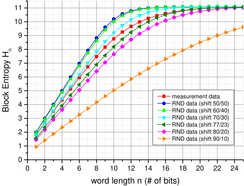
(a) Block entropy $H_{n}$

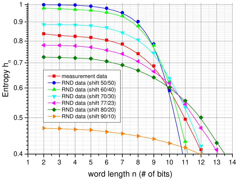
(b) Entropy $h_{n}$

Figure 10: Block entropy $H_{n}$ and entropy $h_{n}$ of the measurement data compared to random distributions with varying skewness. Data set length is constant.

conditional probabilities

Another option to check for deterministic components is to look for recurrent sequences in the signal. Therefore, we calculated the conditional probabilities $P(W^{n}|W^{m})$ with $n=m=1..4$ to look for recurring patterns with a memory of up to 4. This limit applies due to the finite data set size, therefore the total word length $l_{W}=n+m$ for our measurement is restricted to 8. For each word length the conditional probabilities of all possible combinations were calculated giving a matrix of size $n\,\times\,n$. Again we compare to a random signal of the same size as the measurement data set. For a random data set of infinite length one expects an even distribution of conditional probabilities. However, as we compare finite size data sets, the conditional probabilities become nonuniform at higher word lengths as not all combinations are represented equally, cf. Fig. 11(b). The figure displays the deviation from a perfect random distribution, which would show as a 50% gray tile.

The conditional probabilities of the data set deviate substantially from the even distribution the random data provides, cf. Fig. 11(a). The jet is more likely to alternate between left and right transports which is evident by the higher conditional probabilities of alternating binary combinations, ie. $P(W^{n}|1010),P(W^{n}|0101)$. Some combinations with two or more consecutive transfers in the same direction show a higher than average probability, but these are always combined with alternating sequences. Uniform combinations, ie. $P(W^{n}|0000),P(W^{n}|1111)$, are extremely rare events.

The diminished entropy production with increasing word length is caused a preference for alternating transfers which are evidenced by nonuniform conditional probabilities. The signal is more predictable and most common combinations are already covered with lower length words thus the additional words carry less new information.

(a) Measurement data

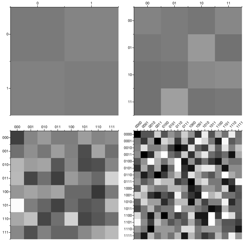
(b) Random distribution

Figure 11: Conditional probabilities for measurement data (a) compared to a random distribution (b). Each tile represents the conditional probability $P(W^{m}|W^{n})$, where $W^{m}$ is plotted on the x-axis and $W^{n}$ is plotted on the y-axis. Word length $l_{W}=1..4$. The grey scale for each plot is centered at the expected probability, i.e. for $l_{W}=2$: $P(W^{m}|W^{n})=0.25$ for all possible combinations. From this value the scale covers $50\%$ deviation, i.e. $l_{W}=2$: black: $P(W^{m}|W^{n})=0.125$, white: $P(W^{m}|W^{n})=0.375$.

Eventually, we compare the results from entropy and LE estimation. For the LE we obtained $\lambda_{+}=0.92$, $\lambda_{-}=-1.43$. For the Shannon entropy we can read off the entropy gain from Fig. 10 (red line and markers) as $h_{KS}=0.82$. Using the Kaplan-Yorke conjecture we should find a coincidence $h\simeq\left<\lambda_{+}\right>$ with a Kaplan-Yorke dimension of 1.92. Given the error sources in the LE estimation and the relatively short time series, we consider this result as a very good coincidence.

IV Discussion and summary

We presented a relatively simple experiment exhibiting complex dynamics, where turbulent mixing reaches out for the nanoscale, at least in one dimension. This renders the flow two–dimensional, however with additional forces acting between the surfaces: disjoining pressure and capillary pressure.

With respect to turbulence, we observe that the relatively low-$Ra$ convection generates a weakly turbulent flow with two prominent rolls. the turbulence mainly can be observed inside the rolls on shorter time scales, whereas transport between the rolls is on a slow scale and shows signs of chaos. To characterize the flow, we take advantage of our measurement capacities, and the color imaging velocimetry (CIV) technique. In addition to the flow field, concluded from Lagrangian trajectories, we obtain local deformation rates which are used to estimate the Lyapunov exponents. With respect to mixing we clearly observe the typical chaotic filamentation. As mentioned in the context of weak turbulence, global mixing on the large scale happens between the left and right convection roll.

We focused on two different methods to quantify the dynamics of the flow: Lyapunov exponents and entropies. Whereas the LE are calculated using small-scale dynamics using CIV, i.e. tracking of small fluid spots, entropies have been calculated using the left-right transport across the separatrix. Qualitatively, these two observations are related by the two “spots” generating the dynamics: the hyperbolic fixed points. They determine the microscopic properties (LE) and as well the transport across the separatrix. Thus, based on dynamical systems principles one expects that both quantities coincide. Given the two different approaches and the very different spatial scales, this coincidence is a formidable cconfirmation of theory.

The presented data is gathered from 8 individual runs of the experiment. Entropy production and conditional probabilities were calculated for the data set and compared to truly random data sets of varying size and skewness. The conditional probabilities show that an alternating pattern of left and right transports is preferred which increases the predictability and lowers the entropy production of the measurement data with respect to equally distributed data. The number of left and right transports in the data is even with a deviation of $2\%$ from the exact left/right randomly equal distribution, which can be accredited to inaccuracy of experimentally obtained data (rod not positioned at the exact center) and limited data set length. Although the entropy production $h_{n}$ is comparable to skewed random distribution with approximately 70/30 shift, these are two unlinked deterministic mechanisms which lead to a decrease of $h_{n}$.

Due to the shortness of the time series, an entropic analysis has errors beond a certain length of the words formed. In order to have a quantitative measure for this length we compare the measurement with numerically determined left/right random sequences without memory. As displayed by the random data sets of varying size a larger data set would yield a higher accuracy in the entropy production rate and conditional probabilitiyes, but the fundamental scaling behaviour remains the same. Thus the statistical evaluation of the measurement data is valid.

Using such kind of numerical validation procedure, we find clearly that the asymmetry found should be attributed to higher-order memory in the data. This is quite plausible, since we are investigating a fluid system, where memory is “built in” for advected particles and so for advected fluid particles, too. The calculated KS-entropy serves as an upper limit to the Lyapunov exponents, which were calculated from the stretching rates. Experimentally, we used color-tracking which focuses on small scales. This area tracking algorithm provides detailed information about the flow field and is adaptable to work on any data of deformable clusters with high enough contrast with respect to their surrounding.

One key question regards the consistence of LE and entropy estimate. We found an astonishingly close result for entropy and LE using Kaplan and Yorkes conjecture. Both agreed within an error of 10%. The values of 0.92 and -1.43 indicate a relatively moderate large-scale mixing which is due to the fact that the setup involves only two main flow regions among which one has to achieve mixing.

However, in practical terms, such nanofluidic devices can be well used as free-standing mixers with very flexible surface properties. The mixing times are then quite fast, since the device dimensions can be miniaturized further. The true advantage lies, in our opinion, in the very good ratio of surface and volume of the film: such a film has an enormous surface, in our setup the ratio was 1:100000, which is probably only achievable with thin films. The free-standing property, finally, allows to avoid problems with solid-liquid interface forces, rather one can focus on a chemically favorite design of the equally treated surfaces.

Generally, we think that with our relatively simple experiment we can touch deep physical questions on the microscopic nature of thin film flows and treat at the same time very practice-oriented topics.

References

- [1] M Abel, L Biferale, M Cencini, M Falcioni, D Vergni, and A Vulpiani. Exit-time approach to -entropy. Physical review letters, 84(26):6002, 2000.
- [2] L.J. Atkins and R.C. Elliott. Investigating thin film interference with a digital camera. American Journal of Physics, 78:1248, 2010.
- [3] E. Aurell, G. Boffetta, A. Crisanti, G. Paladin, and A. Vulpiani. Growth of non-infinitesimal perturbations in turbulence. Phys. Rev. Lett., 77:1262–1265, 1996.
- [4] R Badii and A Politi. Complexity hierarchical structures and scaling in physics, 1997. Cambridge University Press, Cambridge, UK.
- [5] Robert W Batterman and Homer White. Chaos and algorithmic complexity. Foundations of Physics, 26(3):307–336, 1996.
- [6] S. Davey. Enantiomer separation: Selective soap-films. Nature Chemistry, 2010.
- [7] B.V. Derjaguin. Theory of stability of colloids and thin films. Consultants Bureau New York and London, 1989.
- [8] Charles R Doering and John D Gibbon. Applied analysis of the Navier-Stokes equations, volume 12. Cambridge University Press, 1995.
- [9] Thomas Erneux and Stephen H Davis. Nonlinear rupture of free films. Physics of Fluids A: Fluid Dynamics (1989-1993), 5(5):1117–1122, 1993.
- [10] D. Exerowa and P.M. Kruglyakov. Foam and foam films: theory, experiment, application. Elsevier, New York, 1998.
- [11] Paul Frederickson, James L Kaplan, Ellen D Yorke, and James A Yorke. The liapunov dimension of strange attractors. Journal of Differential Equations, 49(2):185–207, 1983.
- [12] J.N. Israelachvili. Intermolecular and surface forces. Academic press London, 1991.
- [13] M.N. Jones, K.J. Mysels, and P.C. Scholten. Stability and some properties of the second black film. Transactions of the Faraday Society, 62:1336–1348, 1966.
- [14] Holger Kantz and Thomas Schreiber. Nonlinear time series analysis, volume 7. Cambridge university press, 2004.
- [15] H. Kellay. Turbulence: Thick puddle made thin. Nature Physics, 7(4):279–280, 2011.
- [16] Henning Krusemann. Lattice Boltzmann Simulation of 2D Thermal Convection , 2012.
- [17] A. Oron, S.H. Davis, and S.G. Bankoff. Long-scale evolution of thin liquid films. Reviews of Modern Physics, 69(3):931–980, 1997.
- [18] Edward Ott. Chaos in dynamical systems. Cambridge university press, 2002.
- [19] JM Ottino. The Kinematics of Mixing. Cambridge Univ Pr, June 1989.
- [20] Eds. Prud’homme R. K., Khan S. A. Foams: Theory, Measurements, and Applications. Dekker, N.Y., 1996.
- [21] G. Reiter. The artistic side of intermolecular forces. Science, 282(5390):888, 1998.
- [22] David Ruelle. Chaotic evolution and strange attractors, volume 1. Cambridge University Press, 1989.
- [23] F. Seychelles, Y. Amarouchene, M. Bessafi, and H. Kellay. Thermal Convection and Emergence of Isolated Vortices in Soap Bubbles. Phys. Rev. Lett., 100(14):144501, 2008.
- [24] S. Stöckle, P. Blecua, H. Möhwald, and R. Krastev. Dynamics of Thinning of Foam Films Stabilized by n-Dodecyl--maltoside. Langmuir, 26 (7):4974–4977, 2010.
- [25] Tamás Tél and Márton Gruiz. Chaotic dynamics: an introduction based on classical mechanics. Cambridge University Press, 2006.
- [26] J. Vermant. Fluid mechanics: When shape matters. Nature, 476(7360):286–287, 2011.
- [27] E. J. W. Verwey and J. T. G. Overbeek. The Theory of the Stability of Lipophobic Colloids. Elsevier, Amsterdam, 1948.
- [28] M. Winkler and M. Abel. Droplet coalescence in 2d thermal convection of a thin film. Journal of Physics Conference Series, 333(1):012018, December 2011.
- [29] M. Winkler and M. Abel. Mixing in thermal convection of very thin free-standing films. Physica Scripta Volume T, 155(1):014020, July 2013.
- [30] M. Winkler, G. Kofod, R. Krastev, S. Stöckle, and M. Abel. Exponentially fast thinning of nanoscale films by turbulent mixing. Physical Review Letters, 110(9):094501, March 2013.
- [31] Lai-Sang Young. Dimension, entropy and lyapunov exponents. Ergodic theory and dynamical systems, 2(01):109–124, 1982.
- [32] P.J. Yunker, T. Still, M.A. Lohr, and AG Yodh. Suppression of the coffee-ring effect by shape-dependent capillary interactions. Nature, 476(7360):308–311, 2011.
- [33] J. Zhang and XL Wu. Velocity intermittency in a buoyancy subrange in a two-dimensional soap film convection experiment. Physical review letters, 94(23):234501, 2005.