High order numerical methods for networks of hyperbolic conservation laws coupled with ODEs and lumped parameter models

Abstract

In this paper we construct high order finite volume schemes on networks of hyperbolic conservation laws with coupling conditions involving ODEs. We consider two generalized Riemann solvers at the junction, one of Toro-Castro type and a solver of Harten, Enquist, Osher, Chakravarthy type. The ODE is treated with a Taylor method or an explicit Runge-Kutta scheme, respectively. Both resulting high order methods conserve quantities exactly if the conservation is part of the coupling conditions. Furthermore we present a technique to incorporate lumped parameter models, which arise from simplifying parts of a network. The high order convergence and the robust capturing of shocks is investigated numerically in several test cases.

1 Introduction

Networks of hyperbolic PDEs arise from the modeling of many different problems, e.g. water and wastewater networks [1, 2, 3], gas pipelines [4, 5, 6], traffic flow [7, 8], simulation of blood flow [9, 10, 11] or cell migration [12]. The description of such networks is based on one dimensional conservation laws along the edges and suitable coupling conditions at the nodes. The simplest type of coupling uses a set of algebraic relations routing the flow between the arcs of the network. In many of the above applications further coupling conditions arise in which an ODE is located in the junction e.g. buffers [13], storage tanks,manholes [4, 3, 2] or the heart [14]. A wide class of such coupling also occurs when so called lumped parameter models are applied to parts of the network [14, 10, 11, 4]. These models arise from simplification of the flow on the edges in regions where a coarser modeling can be afforded.

In all these applications fast and accurate numerical methods are needed. For the one dimensional flow along the edges a huge variety of classical solvers for hyperbolic conservation laws is available [15, 16]. Especially numerical methods of high order accuracy, e.g. WENO, ADER and DG schemes [17, 15, 18], achieve remarkably accurate solutions relative to their computational costs. For the application on networks however mainly first order schemes have been developed. Recently a high order Riemann solver for purely algebraic coupling conditions was presented in [19].

In the present article we introduce two approaches to high order methods for vertices that can involve ODEs in addition to algebraic coupling conditions. The first method follows the Toro-Castro approach of [20, 19]. After solving a classical first order coupling problem linear coupling conditions for the temporal derivatives of the states at the junction are considered. The ODE is incorporated into this procedure by inserting the full Taylor-expansion of its solution into the coupling conditions. The second method adapts the Harten, Enquist, Osher, Chakravarthy approach [20], which solves a series of classical nonlinear Riemann problems. These problems are considered at the supporting points in time of an explicit Runge Kutta scheme, which is used for the discretization of the ODE. In the context of this solver we investigate an efficient high order solver for lumped parameter models. Here we aim to exploit the underlying network structure for the numerical method.

This paper is organized as follows: First we formulate the problem, specify the coupling conditions and define the generalized Riemann problem at a junction. In section 3 we recall the first order solver for such a coupling problem. The high order method of Toro-Castro type is presented in Section 4, the HEOC type solver in section 5. Based on these we describe a modification suited to networks including lumped parameter models. Finally we present convergence studies and several numerical examples in section 7 to show the quality of the schemes presented.

2 Formulation of the problem and coupling conditions

A Network $\mathcal{N}=(\mathcal{E},\mathcal{V})$ consists of a set of edges $\mathcal{E}=\{E_{1},\ldots,E_{\tilde{n}}\}$ which connect the vertices of the set $\mathcal{V}=\{V_{1},\ldots,V_{\tilde{m}}\}$. On each edge $E_{i}$, $i=1,\dots,\tilde{n}$ the quantities $u^{i}(x,t)\in\mathbb{R}^{d_{i}}$ are governed by a hyperbolic conservation law of the form

$$\partial_{t}u^{i}+\partial_{x}f^{i}(u^{i}) =0\$$ (1)

with the flux function $f^{i}:\mathbb{R}^{d_{i}}\rightarrow\mathbb{R}^{d_{i}}$, time $t\in\mathbb{R}^{+}$ and location $x\in\left[0,L_{i}\right]$.

In the following we consider a single vertex $V$ and assume all edges to be oriented outwards, as depicted in Figure LABEL:fig:Edge_orientation_convention.

Figure 1: Edge orientation convention

Starting from this setup, networks of arbitrary shape can be easily constructed by elementary transformations, e.g. [21]. To improve readability we drop the index $j$ for all quantities at the junction, i.e. $w=w^{j}$, and the spatial dependencies of the $u^{i}$s, which are evaluated at $x=0$.

At the vertex $V$ we now assume a coupling of mixed algebraic-ODE type, i.e.

$$\begin{split}\Phi(u^{1}(t),\ldots,u^{n}(t),w)=0\ ,\\ \dot{w}=F(u^{1}(t),\ldots,u^{n}(t),w),\\ u^{i}(t)=u^{i}(0,t)\ .\end{split}$$ (2)

The algebraic coupling conditions are given by the function $\Phi:\bigotimes_{i=1}^{n}\mathbb{R}^{d_{i}}\times\mathbb{R}^{l}\rightarrow\mathbb{R}^{c}$ for $n$ connected edges and the ODE is defined by the flux $F:\bigotimes_{i=1}^{n}\mathbb{R}^{d_{i}}\times\mathbb{R}^{l}\rightarrow\mathbb{R}^{l}$. Coupling conditions of that type arise from the modeling of e.g. storage components as manholes [3] or reservoirs [22], queues [23, 24], as well as from representing parts of complicated networks by so called lumped parameter models [10, 11, 4].

In order to keep the number of coupling conditions constant, the eigenvalues of the Jacobians $\nabla_{u^{i}}f^{i}$ $\lambda^{i}_{l},\ l=1,\dots,d_{i}$ need to be bounded away from zero for all states considered

$$\lambda^{i}_{1}\leq\ldots\leq\lambda^{i}_{d_{i}}\ , |\lambda^{i}_{l}|>\tilde{\epsilon}>0\qquad\forall l=1,\dots,d_{i}\ .$$ (3)

To ensure that the correct number of coupling conditions is provided and that the problem is well posed [25], we require:

$$\det\left(\nabla_{u^{1}}\Phi(u_{g}^{1},\ldots,u_{g}^{n},w_{0})R^{+,1}|\dots|\nabla_{u^{n}}\Phi(u_{g}^{1},\ldots,u_{g}^{n},w_{0})R^{+,n}\right)\neq 0\ ,$$ (4)

where $R^{+,i}=\left[r^{i}_{d_{i}-c_{i}+1}|\dots|r^{i}_{d_{i}}\right]$ denotes the matrix of all eigenvectors of $\nabla_{u^{i}}f^{i}$ which belong to positive eigenvalues.

$$c_{i}=\#\{\lambda^{i}_{j}|\lambda^{i}_{j}>0\}$$ (5)

denotes the number of positive eigenvalues on edge $i$ and $c=\sum_{i=1}^{n}c_{i}$ defines the total number of coupling conditions prescribed by $\Phi$.

3 The generalized Riemann problem at a junction

One central building block for the construction of schemes in the ADER framework is the generalized Riemann problem. In order to develop similar high order methods for networks, a detailed understanding of the generalized Riemann problem at the junction is required. If additionally an ODE is located at the node, we aim to split the problem into two separate ones. On the PDE side we are looking for high order approximations to the Godunov states at the boundaries of the PDE domains, while simultaneously evolving the ODE in the vertex one time step.

In the following we will discuss two variants to tackle this problem. The first is based on the classical ADER approach of Toro-Castro accompanied by a Taylor method for the ODE. The second one utilizes a Harten, Enquist, Osher, Chakravarthy solver for the PDE and a Runge-Kutta scheme for the ODE.

Definition 1

Generalized Riemann problem of order $k$ at a junction:
Consider a algebraic-ODE type coupling (2) of $n$ edges governed by (1). We call such a coupling situation with given initial state of the ODE $w_{0}$ and polynomial Riemann data $u^{i}(x,0)$ of order $k$ a Generalized Riemann problem of order $k$ at the junction

$$\begin{split}\Phi(u^{1}(t),\ldots,u^{n}(t),w(t))&=0\ ,\\ \dot{w}&=F(u^{1}(t),\ldots,u^{n}(t),w(t)),\\ u^{i}(t)&=u^{i}(0,t)\\ u^{i}(x,0)&=\sum\limits_{l=0}^{k-1}p^{i}_{l}\frac{x^{l}}{l!}\\ w(0)&=w_{0}\ .\end{split}$$

Analogously to the classical Riemann problem, the states at the left boundary of the coupled edges $u_{g}^{i}(t)=\lim_{\tau\rightarrow 0+}u^{i}(0,t+\tau)$ are called Godunov states.

3.1 Solving the classical Riemann problem at the junction

Before considering the generalized Riemann problem we investigate the classical Riemann problem at a junction with an ODE, i.e. the setup of definition 1 with $k=1$

$$\Phi(u^{1}(t),\ldots,u^{n}(t),w(t)) =0\ , \dot{w} =F(u^{1}(t),\ldots,u^{n}(t),w(t)),$$

$$u^{i}(t) =u^{i}(0,t) u^{i}(x,0) =p^{i}_{0}$$

$$w(0) =w_{0}\ .$$

In the case without ODE, the Godunov states are constant in time, i.e. $u^{i}_{g}(t)\equiv u^{i}_{g}(0)$ $\forall t\geq 0$. Due to the presence of the ODE the state in the junction can vary over time and thus also the Godunov states $u^{i}_{g}(t)$ change. However for solving the generalized Riemann problem we are only interested in the states at $t\rightarrow 0+$.

Since the solution of the ODE is continuous in time [25] we have $\lim_{t\rightarrow 0+}w(t)=w_{0}$. Knowing the initial state of the ODE, the problem at $t=0+$ reduces to a classical Riemann problem at a junction. This we can solve with the help of the so called Lax-Curves [19, 26].

Solving such a classical Riemann problem at a junction is equivalent to finding a set of states that fulfill the algebraic part of the coupling conditions while being possible Godunov states accessible from the Riemann data on each edge. In order to be such an accessible state they have to lie on the concatenated Lax curves anchored in the right states $u^{i}_{r}=p_{0}^{i}$ [26]:

$$L_{g}^{i}(\xi^{i}_{1},\ldots,\xi^{i}_{c_{i}},u^{i}_{r}) =L_{d_{i}-c_{i}+1}(\xi^{i}_{1},\cdot)\circ\ldots\circ L^{i}_{d_{i}}(\xi^{i}_{c_{i}},u^{i}_{r})\ ,$$

where the number of curves and free parameters $c_{i}$ is given by (5). The operator $\circ$ denotes the concatenation in the last variable, i.e for two functions $g$ and $h$

$$g(\xi_{1},\ldots,\xi_{l},\cdot)\circ h(\xi_{l+1},\ldots,\xi_{m},x) =g(\xi_{1},\ldots,\xi_{l},h(\xi_{l+1},\ldots,\xi_{m},x))\ .$$

Therefore we have to solve the equations

$$\Phi\left(L^{1}_{g}(\xi^{1},u^{1}_{r}),L^{2}_{g}(\xi^{2},u^{2}_{r}),\ldots,L^{n}_{g}(\xi^{n},u^{n}_{r}),w_{0}\right) =0$$ (6)

for the unknowns $\xi^{i}=(\xi^{i}_{1},\ldots,\xi^{i}_{c_{i}})$. The local solvability of this system for states close to $u_{r}$ is assured by condition (4) [26]. Once the parameters $\xi^{i}$ are known, the Godunov states can be determined by evaluating the concatenated Lax-curves

$$u^{i}_{g}(0)=L_{g}^{i}(\xi^{i},u_{r}^{i})\ .$$

Thus the complete set of states at the junction at $t=0+$ is given by $\{u^{1}_{g}(0),\ldots,u^{n}_{g}(0),w_{0}\}$.

4 Generalized Riemann solver of Toro-Castro type

In the ADER framework the Toro-Castro approach provides a procedure to construct a polynomial in time approximating the solution of the generalized Riemann problem at the considered interface. This is achieved by splitting up the problem into one classical non linear Riemann problem and $k-1$ linearized Riemann problems for the temporal derivatives of the Godunov states. An extension of this procedure to junctions without ODEs was presented in [19].

Let a generalized Riemann problem at an ODE junction be given as in definition 1. As a first step we solve the zeroth order classical Riemann problem as described in section 3.1 using the zero order data, i.e. $u_{r}^{i}=p^{i}_{0}$ . Note that once the states at $t=0+$ are known, we can directly evaluate the ODE $\dot{w}(0)=F(u^{1}_{g}(0),\ldots,u^{n}_{g}(0),w(0))$, which already provides some information about the development of $w(t)$.

In a second step we aim to compute the temporal derivatives of the involved states. As in the classical ADER framework, we obtain governing equations for the derivatives by differentiating the conservation laws with respect to $t$ and obtain

$$\partial_{t}(\partial_{t}^{k}{u^{i}})+\nabla f^{i}(u_{g}^{i})\partial_{x}(\partial_{t}^{k}u^{i})+\text{'sources'}=0 k=1,\dots,{k_{max}}\ .$$ (7)

The term ’sources’ encompasses everything that only depends on derivatives of degree $k$ and less. It can be dropped, since it does not immediately act on the Godunov states [15]. These governing equations for the temporal derivatives are linear hyperbolic systems. Therefore the corresponding Lax curves are linear as well. The concatenated Lax curves to a Riemann problem with $\partial_{t}^{k}u_{r}^{i}$ as states on the right hand side have the short form

$$L^{i,k}_{g}(\xi^{i},u_{r})=\partial_{t}^{k}u_{r}^{i}+R^{+,i}\xi_{k}^{i}\ , R^{+,i}=\left[r^{i}_{d_{i}-c_{i}+1}|\ldots|r^{i}_{d_{i}}\right]\ ,$$ (8)

where $r^{i}_{j}$ denotes the eigenvector corresponding to the $j$-th eigenvalue $\lambda_{j}^{i}$ of $\nabla f^{i}(u^{i}_{g})$. Note that (3) still holds as the Jacobian is the same as in the Riemann problem of order zero.

In order to obtain the coupling conditions for the temporal derivatives, we differentiate $\Phi$ with respect to time. The first order derivative of $\Phi$ reads

$$\frac{d}{dt}\Phi(u_{g}^{1},\ldots,u_{g}^{n},w) =0$$

$$\Rightarrow\sum_{l=1}^{n}\nabla_{u_{g}^{l}}\Phi(u_{g}^{1},\ldots,u_{g}^{n},w)\partial_{t}u_{g}^{l}+\nabla_{w}\Phi(u_{g}^{1},\ldots,u_{g}^{n},w)\partial_{t}w =0\ ,$$

where all quantities are evaluated at $t=0$ and $u_{g}^{i}$ denotes the Godunov state at $x=0$ on edge $i$. By inserting the ODE $\partial_{t}w=F(u_{g}^{1},\ldots,u_{g}^{n},w)$ we obtain

$$\nabla_{u}\Phi(u_{g}^{1},\ldots,u_{g}^{n},w)\partial_{t}u_{g}+\nabla_{w}\Phi(u_{g}^{1},\ldots,u_{g}^{n},w)F(u_{g}^{1},\ldots,u_{g}^{n},w) =0$$

$$\nabla_{u}\Phi(u_{g}^{1},\ldots,u_{g}^{n},w)\partial_{t}u+\Psi_{1}(u_{g}^{1},\ldots,u_{g}^{n},w) =0\ .$$ (9)

The function $\Psi_{1}$ only depends on states at $t=0$ and not on any temporal derivative. Thus we have a linear system governing the temporal derivatives of the Godunov states at the junction. Here and in the following we assume the coupling conditions $\Phi$ to be sufficiently differentiable, otherwise we consider the usage of high order schemes not appropriate.

For the derivatives of orders $k\geq 2$ additional terms arise, which we summarize as $\tilde{\Psi}_{k}$

$$\nabla_{u}\Phi(u_{g}^{1},\ldots,u_{g}^{n},w)\partial_{t}^{k}u_{g}+\tilde{\Psi}_{k}(u_{g},\partial_{t}u_{g},\ldots,\partial_{t}^{k-1}u_{g},w,\partial_{t}w,\ldots,\partial_{t}^{k}w)=0\ .$$

Note that these lower order terms can not be dropped as in the classical ADER framework, i.e. equation (7), since we can not expect that it acts delayed in any form. It is easy to see that $\tilde{\Psi}_{k}$ only depends on lower order derivatives of $u_{g}$ but still on all $k$ derivatives of $w$. This we can reduce by using the derivative of the ODE itself

$$\begin{split}\partial_{t}^{k}{w}&=\partial_{t}^{k-1}F(u^{1}_{g}(t),\ldots,u^{n}_{g}(t),w)\\ &=\Xi(u^{1}_{g},\partial_{t}u^{1}_{g},\ldots,\partial_{t}^{k-1}u^{1}_{g},\ldots,u^{n}_{g},\partial_{t}u^{n}_{g},\ldots,\partial_{t}^{k-1}u^{n}_{g},w,\partial_{t}w,\ldots,\partial_{t}^{k-1}w)\ .\end{split}$$ (10)

Thus we end up with a linear equation for $\partial_{t}^{k}u_{g}$ which only requires derivatives of lower order than $k$

$$\nabla_{u}\Phi(u_{g}^{1},\ldots,u_{g}^{n},w)\partial_{t}^{k}u_{g}+\Psi_{k}(u_{g},\partial_{t}u_{g},\ldots,\partial_{t}^{k-1}u_{g},w,\partial_{t}w,\ldots,\partial_{t}^{k-1}w)=0\ .$$ (11)

Finally we can use this expression to obtain all the temporal derivatives of $u_{g}$ iteratively, by starting with the first order equation (9) and successively solving (11) in increasing order of $k$.

To solve each of these systems (11), we proceed as in the zeroth order case. The temporal derivatives of $u_{g}$ are governed by a linear conservation law (7) and coupled by a set of linear coupling conditions (11). Thus we insert the concatenated linear Lax-curves (8) with the free parameter $\xi^{i}_{k}$

$$\sum_{i=1}^{n}\nabla_{u^{i}}\Phi(u_{g}^{1},\ldots,u_{g}^{n},w)\left(R^{+,i}\xi_{k}^{i}+\partial_{t}^{k}u^{i}_{r}\right)+\Psi_{k} =0$$

$$\Rightarrow\sum_{i=1}^{n}\nabla_{u^{i}}\Phi(u_{g}^{1},\ldots,u_{g}^{n},w)R^{+,i}\xi_{k}^{i}+\sum_{i=1}^{n}\nabla_{u^{i}}\Phi(u_{g}^{1},\ldots,u_{g}^{n},w)\partial_{t}^{k}u^{i}_{r}+\Psi_{k} =0\ .$$

By introducing the notations

$$a_{i} =\nabla_{u^{i}}\Phi(u_{g}^{1},\ldots,u_{g}^{n},w)R^{+,i}\ , A =\left(a_{1}|a_{2}|\ldots|a_{n}\right)\ ,$$

$$\xi_{k} =\begin{pmatrix}\xi_{k}^{1}&\xi_{k}^{2}&\ldots&\xi_{k}^{n}\end{pmatrix}^{T}\ , \partial_{t}^{k}u_{r} =\begin{pmatrix}\partial_{t}^{k}u_{r}^{1}&\partial_{t}^{k}u_{r}^{2}&\ldots&\partial_{t}^{k}u_{r}^{n}\end{pmatrix}^{T}\ ,$$

this linear system can be written as

$$A\xi_{k}+\nabla_{u}\Phi(u_{g}^{1},\ldots,u_{g}^{n},w)\partial_{t}^{k}u_{r}+\Psi_{k} =0\ .$$ (12)

The matrix $A$ is exactly the one in (4) considered for the well-posedness of the coupling conditions. Since we have $\det A\neq 0$, we can solve for the unknowns $\xi_{k}$

$$\xi_{k} =A^{-1}\left(-\nabla_{u}\Phi(u_{g}^{1},\ldots,u_{g}^{n},w)\partial_{t}^{k}u_{r}-\Psi_{k}\right)\ .$$

In order to evaluate this expression, the temporal derivatives of the states within the edges $\partial_{t}^{k}u_{r}$ are needed. Analogous to the classical ADER approach we start with a WENO reconstruction of the spatial initial data. Since we are at the boundary of a domain, we have to use an one-sided reconstruction of type [27] to obtain spatial derivatives $\partial_{x}^{k}u_{r}$ at the junction. These we can transform into temporal derivatives $\partial_{t}^{k}u_{r}$ using the Cauchy-Kowalewski or Lax-Wendroff procedure [15, 27].

Note that carrying out the Cauchy-Kowalewski procedure on the basis of the zeroth order Godunov state is not strictly necessary, but does not cause any additional computational costs either. It is however necessary to make the scheme revert to the classical Toro-Titarev ADER scheme for one on one coupling, as we showed in [19]. Once the values of $\xi_{k}$ are determined, we can evaluate the Lax-curves (8) to obtain the temporal derivatives of the Godunov states $\partial_{t}^{k}u_{g}$. With these we can directly build a polynomial approximation of $u_{g}(t)$ at the interfaces of the junction.

An approximation to the states of the ODE can now be constructed easily. Since for the computation of $\partial_{t}^{k}u_{g}$ we already determined all the derivatives of $w$ using equation (10), we just combine these to a Taylor series approximating $w(t)$.

The scheme derived from the Toro-Castro type solver for the generalized Riemann problem at the junction with ODE can be summarized as follows:

1. Obtain GRP data at the junction via one-sided polynomial reconstruction.

2. Solve the zeroth order Riemann problem at the junction, as described in section 3.1.

3. Apply the Cauchy-Kowalewski procedure to obtain temporal polynomials as input data.

4. Solve the generalized Riemann problem at the junction, as described above.

5. Approximate the fluxes across cell interfaces at the junction using the temporal derivatives of the Godunov states.

6. Update the state $w$ in the junction by applying a Taylor scheme of order $k$.

7. Fill the ghost cells at the junction if needed.

8. Run a high order finite volume scheme e.g. ADER to compute the fluxes across interior cell interfaces.

A detailed description how to fill the ghost cells, if needed, is given in [19].

At this point we note that the above procedure requires, besides the Cauchy-Kowalevsky procedure, the derivatives up to order $k$ of the ODE as well as those of the coupling conditions.

5 Generalized Riemann solver at an ODE junction Harten, Enquist, Osher, Chakravarthy type

A popular alternative to the Toro-Castro approach for solving generalized Riemann problems is the Harten, Enquist, Osher, Chakravarthy solver [20]. Instead of solving the linear governing equations for the derivatives, it uses several classical Riemann problems at different points in time to achieve a high order approximation of the flux. Here we present a HEOC type solver for junctions, which is accompanied by a Runge-Kutta scheme for the ODE.

In the classical HEOC approach, the solution of a generalized Riemann problem is approximated by the solutions of a sequence of classical Riemann problems. First we fix a quadrature rule according to the desired order of the scheme. Then the classical Riemann problem at $t=0$ is solved. Based on its solution the spatial data on each side of the interface can be flipped into the time domain using the Cauchy-Kowalevsky procedure. These polynomials can be evaluated at the supporting points of the given quadrature rule, such that a series of classical Riemann problems arises. Their solutions serve as approximation of the states at the interface at these points in time. This information can be inserted into the quadrature rule to obtain a high order approximation of the fluxes at the interface. In Figure 2 a schematic representation of this procedure is shown.

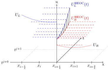
Figure 2: HEOC schematic.

In the following we adapt this approach to generalized Riemann problems at junctions with ODEs. Before considering the fluxes of the PDE, we start with the numerical method for the ODE. Here we choose an explicit Runge-Kutta scheme which is at least accurate of order $k$. Usually the coefficients of RK-schemes are given in form of a Butcher array

$$\bar{B} =\left(\begin{array}[]{c|c}\bar{c}&\bar{A}\\ \hline\cr&\bar{b}\end{array}\right)\ ,$$

such that for an ODE $\dot{w}=F(t,w)$ the update formula reads

$$w_{n+1} =y_{n}+\Delta t\sum_{j=1}^{s}\bar{b}_{j}k_{j}\ , k_{i} =F(t_{n}+\bar{c}_{i}\Delta t,w_{n}+\Delta t\sum_{j=1}^{i-1}\bar{a}_{ij}k_{j})\ .$$ (13)

At this point we note that each RK-scheme of order $k$ naturally provides a quadrature formula of order $k$ with the supporting points $c_{i}\Delta t$, such that

$$\int_{0}^{\Delta t}\tilde{F}(\tau)d\tau=\Delta t\sum_{j=1}^{s}\bar{b}_{j}\tilde{F}(t_{n}+\bar{c}_{i}\Delta t)+\mathcal{O}(\Delta t^{k+1})\ .$$

In the following we will use exactly these intermediate time levels $t_{l}=c_{l}\Delta t$ to set up the HEOC coupling procedure.

Before considering higher order terms we have to solve the classical Riemann problem at $t=0$,

$$\Phi(p^{1}_{0},\ldots,p^{n}_{0},w_{0})=0\ .$$

Following the procedure described in 3.1 we obtain the values of Godunov states at $t=0$, i.e. $u^{1}_{g}(0),\ldots u^{n}_{g}(0)$. Using these values we can transform the spatial data from a one-sided polynomial reconstruction into temporal data via Cauchy-Kowalevsky procedure. Thus for each connected edge we obtain a temporal polynomial of the form

$$u^{i}_{r}(t) =\sum\limits_{l=0}^{k_{\max}-1}p^{i,\text{time}}_{l}\frac{t^{l}}{l!}\$$

as input data for the generalized Riemann problem at the junction. With these values available, we now aim to solve the classical Riemann problems at the time levels $t_{l}$

$$\Phi(u^{1}_{g}(t_{l}),\ldots,u^{n}_{g}(t_{l}),w(t_{l})) =0\ .$$ (14)

In order to apply the technique of section 3.1 we have to provide some approximation for the value of $w(t_{l})$. This is naturally provided by the RK-scheme as in the second formula of (13)

$$w_{l} =w_{0}+\Delta t\sum\limits_{i=1}^{l-1}\bar{a}_{l,i}k_{i}\ .$$ (15)

As in the classical RK methods, the value $w_{l}$ is not necessarily an approximation of very high order, but chosen in such a way that in the final update the desired order is obtained. Note that for the evaluation of the stages $k_{i}=F(t_{i},u_{g}^{1}(t_{i}),\ldots,u_{g}^{n}(t_{i}),w_{i})$ $i=1,\dots,l-1$ values of $w_{i}$ and $u_{g}(t_{i})$ are needed. But since we have chosen an explicit RK-scheme, only data from the previous $l-1$ stages is used.

Inserting (15) into (14) we obtain

$$\Phi(u^{1}_{g}(t_{l}),\ldots,u^{n}_{g}(t_{l}),w_{l}) =0\$$

and can solve this classical Riemann problem for the Godunov states at $t_{l}$.

Once all Riemann problems are solved successively, we can compose the solutions to determine the fluxes of the conservation laws and to update the ODE

$$f^{i}_{-\frac{1}{2}} =\sum\limits_{l=1}^{k}\bar{b}_{l}f^{i}(u^{i}_{g}(t_{l}))\ , w(t+\Delta t) =w(t)+\Delta t\sum\limits_{l=1}^{k}\bar{b}_{l}k_{l}\ .$$ (16)

The coefficients $b_{l}$ in both formulas are those of the RK-scheme (13) and the stages $k_{l}$ have been already computed for the formula (15). The complete scheme can be summarized as

1. Obtain GRP data at the junction via one-sided polynomial reconstruction.

2. Solve the zeroth order Riemann problem at the junction, as described in section 3.1.

3. Apply the Cauchy-Kowalewski procedure to obtain temporal polynomials as input data.

4. Solve the classical Riemann problems at the times $t_{l}$ as described above.

5. Approximate the fluxes across cell interfaces at the junction using the Godunov states at the time levels $t_{l}$.

6. Update the state $w$ in the junction by applying the RK-scheme of order $k$.

7. Run a high order finite volume scheme to compute the fluxes across interior cell interfaces.

One advantage of this approach is that neither the derivatives of the coupling conditions nor those of the ODE are needed. Thus the only symbolic manipulation necessary is the CK procedure, which is required for ADERs scheme inside the domain anyway. Furthermore we can solve the ODE with some classical RK-scheme, which is helpful especially for complicated or large ODEs e.g. those that arise from lumped parameter models.

The main disadvantage of this approach is the higher computational costs, since several nonlinear Riemann problems have to be solved instead of just one nonlinear and a couple of linear ones. Furthermore we do not have enough information at the interfaces to fill possible ghost cells at the computational boundary. Thus for the reconstruction in the interior of the domain but close to the boundary we use a reconstruction with variable stencil lengths [27].

5.1 Conservation of quantities

In many applications and their corresponding models some quantities are conserved in the complete network, e.g. the total mass [24, 2, 6, 10]. This is not only established via the conservation laws on the edges, but also due to a careful choice of the coupling conditions and the ODE in the junction.

Since the conservation is guaranteed to be exact in the interior of the edges by the numerical scheme, it is desirable that also the coupling procedure is conservative. The first order junction solver in section 3.1 is conservative, since the same Godunov states are used in the coupling conditions as well as for the computation of the fluxes across the interfaces. If the ODE is updated by an explicit Euler scheme, its update relies on the same values as the coupling condition. Clearly at the junction the conservation is only guaranteed up to the precision of the numerical method used to solve the nonlinear system arising from the coupling conditions.

In case of no ODE in the junction it has been proven in [19] that the Toro-Castro approach also conserves the selected quantities. This proof can be easily modified such that it fits the current setting. We just have to take care that the ODE is updated with exactly the same numerical values as those arising in the coupling procedure. Therefore it is mandatory to use a Taylor scheme for the ODE.

For the HEOC approach at any intermediate time level $t_{l}$ a classical Riemann Problem at a junction is considered. If now some quantity is conserved in the underlying system, at each of these Riemann problems the fluxes of the resulting Godunov states and the flux of the ODE balance exactly. Since we choose the identical $\bar{b}_{l}$s for the flux integration and the RK-scheme (16), this also holds for the final updates in the PDEs and the ODE.

5.2 Source-terms

In many applications the conservation law (1) is replaced by a balance law via introducing source terms. These usually do not affect the coupling procedure [2]. If we have a numerical scheme at hand that is capable to treat the source terms properly and include the sources into the Cauchy-Kowalevsky -procedure, all the above methods can be applied. Since the lower order terms in (7) are dropped, the sources do neither change the Lax curves nor the governing equations of the higher order derivatives.

6 Lumped Parameter Models

In a lot of real world applications the dimensions of the network exceed the affordable computational effort, e.g. capillaries in the circulatory system. At the same time a detailed description of the flow is only needed in certain areas of the network. Therefore it is often convenient to describe some parts of the network by simpler models. A wide class of such reduced models are the so called lumped parameter models, which are used to describe e.g. the human circulatory system [10, 11] or gas networks [4].

In this section we explain a process to construct high order schemes for hybrid models of networks containing hyperbolic conservation laws and lumped parameter models. To have access to such a process in an algorithmic framework is especially of interest in the context of dynamical switching between highly resolved and reduced models [4].

Consider one edge in the network of length $L$ with a conservation law

$$\partial_{t}u(t,x)+\partial_{x}\left(f(u(t,x))\right)=0\ .$$

Following the approach proposed in [11], a lumped parameter model is obtained by averaging over the whole spatial domain, i.e.

$$\partial_{t}\left(\underbrace{\frac{1}{L}\int_{0}^{L}u(t,x)d_{x}}_{=:U}\right) +\frac{1}{L}\left[f(\underbrace{u(t,L)}_{=:U_{g}^{r}})-f(\underbrace{u(t,0)}_{=:U_{g}^{l}})\right]=0$$ (17)

$$\Rightarrow U^{\prime} =F(U,U_{g}^{l},U_{g}^{r})\ .$$

Thus the averaged state $U$ is governed by a simple ODE with the unknown Godunov states at the left and right boundary $U_{g}^{l}$ and $U_{g}^{r}$. If such an edge is connected to a node in the network, these values will be determined when solving the associated coupling conditions. The coupling procedure from section 3.1 remains unchanged by the averaging process, but the Lax curve have now to be anchored at the only accessible state $U$. This implies, if complete sections of the network are simplified to lumped parameter models in the above manner, that the PDEs are not coupled to a simple ODE but to a differential algebraic equation (DAE). The components of the lumped region can be summarized as follows

$$w^{\prime} =F(w,u_{g})$$ ODE part, originates from lumped edges and ODE parts already present in vertices, (18)

$$\Phi(u_{g},w) =0$$ Algebraic constraints stem from the coupling conditions of the vertices, (19)

$$u_{g}-L(w,\xi) =0$$ Lax curve condition to connect the Godunov states with the internal states.

Note that here $w$ contains the averaged states of all lumped edges in a connected area and all possible ODE states in the junctions of this region.

From a numerical point of view the algebraic constraints (19) do enforce the usage of an appropriate solver of DAEs in the junction, e.g. modified RK schemes [28]. In the following however we want to present a technique to construct a high order solver using the underlying network structure of the LPM.

Since the lumped areas might be very large or vary in time, due to switching between the models, we base the following procedure on the HEOC approach. As in section 5 we first apply polynomial reconstruction to obtain spatial data on the PDE-edges. For each vertex in the lumped parts of the network we solve the following zeroth order coupling problem as (6)

$$\Phi(u^{1}_{g},\ldots,u^{i}_{g},w_{0})=0 u^{i}_{r}=\begin{cases}p^{i}_{0}&\text{edge is equipped with a PDE}\\ U^{i}_{0}&\text{edge model is lumped}\end{cases}\quad.$$ with

This yields the Godunov states on the PDE edges at $t=0$, which are used to flip the data into time by Cauchy-Kowalevsky procedure, providing polynomials $u^{i,\text{time}}(t)$. We repeat this step for each stage $l$ of the RK-scheme in the HEOC approach and for each vertex in the lumped network, i.e. we solve the zeroth order coupling problem at $t_{l}=c_{l}\Delta t$,

$$\Phi(u^{1}_{g},\ldots,u^{i}_{g},w_{l})=0 u^{i}_{r} =\begin{cases}u^{i,\text{time}}(t_{l})&\text{If the edge in question is a PDE}\\ U^{i}_{l}&\text{if the edge in question is lumped}\end{cases}\quad.$$ with

The states $U^{i}_{l}$ are known from the previous stage of the RK-scheme and the new ones are obtained by

$$U^{i}_{l+1}=U_{0}+\Delta t\sum\limits_{i}^{l}\bar{a}_{l+1,i}k^{U}_{i}\ , w^{j}_{l+1}=w_{0}+\Delta t\sum\limits_{i}^{l}\bar{a}_{l+1,i}k^{w}_{i}\ ,$$

where $k_{i}^{U}$ and $k_{i}^{w}$ are the components of the intermediate values $k_{i}$ for the lumped edges or the ODEs in the junctions respectively.

With this procedure we can keep the full network structure, such that we can easily select any part of this network and switch between the simplified and the more accurate model. The scheme can be summarized by the following steps

1. Obtain GRP data at the junction via one-sided polynomial reconstruction.

2. Solve the zeroth order Riemann problem at the junction, as described in section 3.1.

3. Apply the Cauchy-Kowalewski procedure to obtain temporal polynomials as input data.

4. Compute each stage of the RK-scheme as described above.

5. Approximate the fluxes across cell interfaces at the junction using the Godunov states at the time levels $t_{l}$.

6. Update the state $w$ in the junction by applying the RK-scheme of order $k$.

7. Run a high order finite volume scheme to compute the fluxes across interior cell interfaces.

6.1 Source-terms in lumped parameter models

Source terms can be treated in a straight forward way, since they do not affect the coupling procedure. Only when particular steady states should be preserved, the averaging process in (17) has to be adapted accordingly. In case of a balance law we obtain

$$\partial_{t}u(t,x)+\partial_{x}\left(f(u(t,x))\right) =S(u(t,x))$$

$$\Rightarrow\partial_{t}U+\frac{1}{L}\left[f(U_{g}^{r})-f(U_{g}^{l})\right] =\frac{1}{L}\int_{0}^{L}S(u(t,x))\approx\tilde{S}(U)\$$

For example in the case of the shallow water equations (21) a huge variety of well-balanced numerical schemes has been developed in order to incorporate the bottom elevation in a suitable manner e.g. [29, 30, 31]. In this particular situation the approximation made to obtain $\tilde{S}$ reads as

$$\frac{1}{L}\int_{0}^{L}-gh\partial_{x}b \approx-g\bar{h}\frac{b(L)-b(0)}{L}\ ,$$ (20)

where $h$ denotes the water level, $b$ the bottom elevation and $g$ the gravitational acceleration.

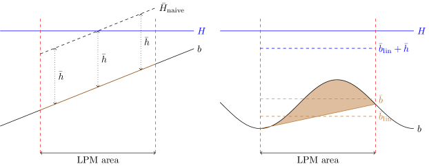
Figure 3: Problems arising from naive lumping. Left: Scheme can become very unbalanced. Right: Conservation of mass violated.

As illustrated in figure 3 an independent treatment of flux an source can not lead to a method preserving steady states. Therefore we have to apply a reconstruction technique to the values $U$, which follows the bottom topography. This so called hydrostatic reconstruction [30] is a well known tool in this context. Thus whenever bottom elevation is considered we will apply the hydrostatic reconstruction on lumped edges in order to capture the ’lake at rest’ correctly.

A further detail concerning this particular steady state is also depicted in figure 3. If an initial condition for the PDE model is provided on the network, the initial conditions of the lumped parameter model are obtained by the averaging process in (17). Since in (20) the bottom elevation is linearized, possible errors have to be compensated in the initial values of $U$. In the following we will just add the missing amount of water artificially to the initial states of the LPM model by modifying the reconstruction to

$$U =\frac{1}{L}\int_{0}^{L}u(x)dx+\left(\frac{1}{L}\int_{0}^{L}b(x)dx-\frac{1}{2}(b(L)+b(0))\right)\ .$$

7 Numerical Examples

In this section we investigate the above presented numerical methods in different test cases. As conservation law along the edges we choose the shallow water equations

$$\begin{aligned} \partial_{t}h+\partial_{x}q&=0\\ \partial_{t}q+\partial_{x}\left(\frac{q^{2}}{h}+\frac{1}{2}gh^{2}\right)&=0\ .\end{aligned}$$ (21)

$h$ denotes the depth of the water and $q$ is the discharge in $x$ direction. $g=9.81$ is the gravitational acceleration.

As coupling conditions in the junctions we consider two different sets of equations. The first one is the so called ’equal heights’ coupling, which reads for $n$ connected edges

$$\begin{split}\sum_{i=1}^{n}q_{i}&=0\ ,\\ h_{1}-h_{i}&=0\quad 2\leq i\leq n\ .\end{split}$$ (22)

The first equation states the conservation of mass at the junction. The remaining $n-1$ equations force all heights at the junction to be at the same level.

The second set of coupling conditions involve an ODE at the junction. Here we consider a storage tank or manhole at the coupling point, which is modeled by

$$\dot{h}_{m} =\frac{Q_{m}}{A_{m}}$$

$$\dot{Q}_{m} =\frac{gA_{m}}{h_{m}}\left(\frac{1}{2g}\frac{q_{1}^{2}}{h_{1}^{2}}+h_{1}-\left(\frac{1}{2g}\frac{Q_{m}^{2}}{A_{m}^{2}}+h_{m}\right)\right)\ .$$ (23)

The two states are the vertical water level in the tank $h_{m}$ and the discharge $Q_{m}$ flowing into the volume. The constant $A_{m}$ is the horizontal cross sectional area of the storage tank. It is important that this model is always accompanied by the following set of coupling conditions

$$\begin{aligned} \sum_{i=1}^{n}q_{i}+Q_{m}&=0\ ,\\ \frac{1}{2g}\frac{q_{1}^{2}}{h_{1}^{2}}+h_{1}-\left(\frac{1}{2g}\frac{q_{i}^{2}}{h_{i}^{2}}+h_{i}\right)&=0\qquad 2\leq i\leq n\ .\end{aligned}$$

The first equation again ensures the conservation of total mass in the coupled system. The following $n-1$ equations state the equality of the so called hydraulic heads or energy levels. As this name indicates these conditions provide the conservation of the total energy at the junction in case of smooth solutions [6, 2]. The total energy in the coupled system is conserved due to equation (23) in the storage model [2]. Here we further note that (23) does not depend on the choice of the related edge since all hydraulic heads coincide.

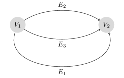
Figure 4: Split circle network.

In the following convergence studies, we use a simple network consisting of three edges and two nodes, as shown in Figure 4. All edges are of the same length $L=25$ and in both nodes a storage tank with $A_{m}=1$ is placed. The initial data used for convergence studies needs not only to be smooth along the edges, but also has to satisfy the coupling conditions and its temporal derivatives up to the order of the schemes to be investigated. In the following we choose lake at rest like states at the junctions and a sufficiently smooth transition between their two water levels. This can be achieved by $q_{i}(x,0)=0$ $i=1,2,3$ and polynomial states of degree $15$ for $h_{i}$ which are determined by the constraints

$$h_{i}(0,0)=2\ ,\quad\partial_{x}^{k}h_{i}(0,0)=0\ , h_{i}(L,0)=3\ ,\quad\partial_{x}^{k}h_{i}(L,0)=0\ ,\quad k=1,\dots,7\ .$$

The initial states of the ODEs are also at rest, i.e. $w^{1}(0)=(2,0)^{T}$ and $w^{2}(0)=(3,0)^{T}$.

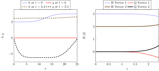
Figure 5: Initial Data and solution for the convergence studies 7.1 and 7.2. PDE states on the edges to the left, ODE states in the vertices on the right side.

In Figure 5 we show initial states as well as the reference solution for the PDEs on the left side, on the right hand side are the states of the ODEs in the nodes for $t\in[0,2.4]$. The computation of the reference solution was performed by a scheme of order $8$ on a grid of $800$ cells per edge.

In all numerical examples the time step $\Delta t$ is synchronized in the complete network according to a CFL number $0.95$. The stability bounds of the ODEs are always less restrictive than those of the PDEs.

7.1 Convergence study Toro-Castro

The first convergence tests we perform for the Toro-Castro solver which is described in section 4. In Figure 6 the $L^{1}$ and the $L^{\infty}$-error at $t=2.4$ are plotted against the reciprocal of the cell width $\Delta x$. Furthermore the $L^{2}$-errors of the involved ODEs are shown.

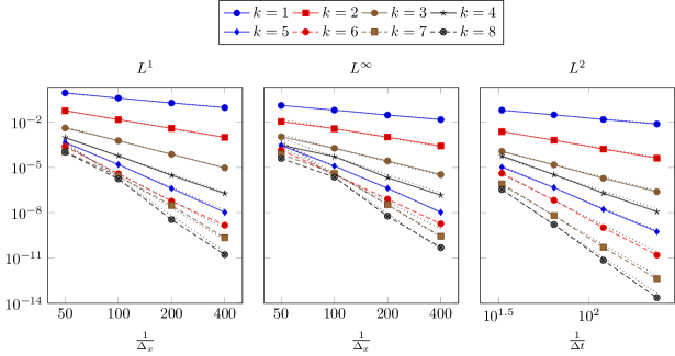
Figure 6: Convergence study 7.1: Splitcircle TT solver in $L^{1}$ and $L^{\infty}$ norm for the edges, $L^{2}$ norm for the ODEs.

Additionally for selected orders $k$ the errors and rates of convergence are given in Table 1.

	$k=2$		$k=4$		$k=5$		$k=6$		$k=8$
PDE $L^{1}$ norm
N	$L^{1}$	$O_{L^{1}}$	$L^{1}$	$O_{L^{1}}$	$L^{1}$	$O_{L^{1}}$	$L^{1}$	$O_{L^{1}}$	$L^{1}$	$O_{L^{1}}$
50	5.51e-02		9.32e-04		4.34e-04		2.37e-04		1.02e-04
100	1.44e-02	1.94	5.71e-05	4.03	1.52e-05	4.83	3.81e-06	5.96	1.71e-06	5.89
200	3.79e-03	1.92	2.95e-06	4.28	4.04e-07	5.24	5.77e-08	6.04	3.45e-09	8.96
400	9.61e-04	1.98	1.86e-07	3.98	1.05e-08	5.27	1.46e-09	5.31	1.67e-11	7.69
PDE $L^{\infty}$ norm
N	$L^{\infty}$	$O_{L^{\infty}}$	$L^{\infty}$	$O_{L^{\infty}}$	$L^{\infty}$	$O_{L^{\infty}}$	$L^{\infty}$	$O_{L^{\infty}}$	$L^{\infty}$	$O_{L^{\infty}}$
50	1.06e-02		2.89e-04		2.77e-04		1.38e-04		3.85e-05
100	3.59e-03	1.56	5.13e-05	2.50	1.21e-05	4.51	3.43e-06	5.34	2.23e-06	4.11
200	1.01e-03	1.83	2.06e-06	4.64	4.17e-07	4.86	7.81e-08	5.45	5.85e-09	8.57
400	2.58e-04	1.96	1.43e-07	3.85	1.05e-08	5.30	1.83e-09	5.42	4.90e-11	6.90
ODE $L^{2}$ norm
N	$L^{2}$	$O_{L^{2}}$	$L^{2}$	$O_{L^{2}}$	$L^{2}$	$O_{L^{2}}$	$L^{2}$	$O_{L^{2}}$	$L^{2}$	$O_{L^{2}}$
33	2.31e-03		5.62e-05		1.02e-05		4.02e-06		3.35e-07
64	6.22e-04	1.98	3.27e-06	4.30	4.53e-07	4.70	6.64e-08	6.19	1.63e-09	8.05
120	1.60e-04	2.16	1.94e-07	4.50	1.67e-08	5.25	1.02e-09	6.64	7.02e-12	8.66
237	4.01e-05	2.04	1.17e-08	4.13	5.53e-10	5.01	1.56e-11	6.14	2.35e-14	8.37

Table 1: Convergence study 7.1: Convergence rates splitcircle with TT solver.

All numerical solutions converge with the expected order.

7.2 Convergence study Harten, Enquist, Osher, Chakravarthy

For the HEOC-coupling procedure we repeat the same test for schemes up to order $k=6$. The $L^{1}$- and $L^{\infty}$ errors for the PDEs and the $L^{2}$-errors of the ODEs are shown in in Figure 7. The precise values and the corresponding convergence rates are presented in Table 2.

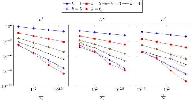
Figure 7: Convergence study 7.2: Splitcircle HEOC solver in $L^{1}$ and $L^{\infty}$ norm for the edges, $L^{2}$ norm for the ODEs.

	$k=2$		$k=4$		$k=5$		$k=6$
PDE $L^{1}$ norm
N	$L^{1}$	$O_{L^{1}}$	$L^{1}$	$O_{L^{1}}$	$L^{1}$	$O_{L^{1}}$	$L^{1}$	$O_{L^{1}}$
50	4.39e-02		6.80e-04		1.38e-04		1.94e-04
100	1.13e-02	1.95	5.21e-05	3.71	5.09e-06	4.76	3.48e-06	5.80
200	3.03e-03	1.90	2.97e-06	4.13	1.48e-07	5.10	1.74e-08	7.64
400	7.69e-04	1.98	2.02e-07	3.88	3.63e-09	5.35	3.18e-10	5.78
PDE $L^{\infty}$ norm
N	$L^{\infty}$	$O_{L^{\infty}}$	$L^{\infty}$	$O_{L^{\infty}}$	$L^{\infty}$	$O_{L^{\infty}}$	$L^{\infty}$	$O_{L^{\infty}}$
50	1.05e-02		3.49e-04		6.87e-05		1.40e-04
100	3.22e-03	1.70	4.59e-05	2.93	5.97e-06	3.52	9.02e-06	3.96
200	8.73e-04	1.88	1.62e-06	4.83	1.77e-07	5.08	2.65e-08	8.41
400	2.22e-04	1.98	1.20e-07	3.76	3.52e-09	5.65	1.50e-09	4.14
ODE $L^{2}$ norm
N	$L^{2}$	$O_{L^{2}}$	$L^{2}$	$O_{L^{2}}$	$L^{2}$	$O_{L^{2}}$	$L^{2}$	$O_{L^{2}}$
33	2.86e-03		1.06e-05		7.86e-06		6.32e-06
64	8.16e-04	1.89	1.25e-06	3.24	2.79e-07	5.04	3.85e-07	4.22
120	2.13e-04	2.13	2.90e-07	2.32	9.12e-09	5.44	1.23e-09	9.14
237	5.40e-05	2.02	2.08e-08	3.87	2.63e-10	5.21	8.86e-12	7.25

Table 2: Convergence study 7.2: Convergence rates Splitcircle HEOC solver.

The errors are within the same range as those of the Toro-Castro method and all solutions converge with the predicted order.

7.3 Convergence study Lumped Parameter Model

The final convergence test addresses lumped parameter models.

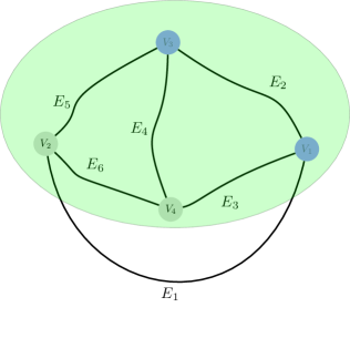
Figure 8: Diamond network. The blue vertices $V_{1}$ and $V_{3}$ are energy conserving manholes, i.e. ODE vertices, the rest algebraic equal height coupling vertices. The green area is lumped resulting in a network of one remaining Edge $E_{1}$ and an LPM vertex with a state of 14 components.

Therefore we consider a network consisting of six edges and four vertices as depicted in Figure 8. In the two junctions $V_{2}$ and $V_{4}$ equal height coupling is applied, while in $V_{1}$ and $V_{3}$ two manholes with $A_{m}=1$ are located. The lumping of section 6 is applied to the whole network except $E_{1}$, i.e. the green colored region.

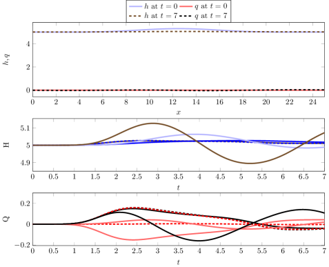
Figure 9: Convergence study Diamond LPM 7.3, initial data and solutions: From top to bottom: PDE initial data on $E_{1}$, ODE components of height type and ODE components of impulse type.

As initial conditions we choose water at rest $q_{i}(x,0)\equiv 0$ $i=1,\dots,6$ with the constant water level $h_{i}(x,0)\equiv 0$, $i=2,\dots,6$ , except for the first edge. There we take as data a polynomial of degree $14$ such that

$$h_{1}(0,0) =5\ , h_{1}(\frac{L}{2},0)=5.3\ , h_{1}(L,0) =5\ ,$$

$$\partial_{x}^{k}h_{1}(0,0) =0\ , \partial_{x}^{k}h_{1}(L,0) =0\quad\forall k=1,\dots,6$$

hold. In Figure 9 initial data and solutions are shown. For edge $E_{1}$ only the solution at $t=0$ and $t=7$ are plotted, whereas the states of all ODEs are shown on the full time interval $[0,7]$.

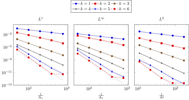
Figure 10: Convergence study diamond LPM 7.3, $L^{1}$ and $L^{\infty}$ norm for the edge, $L^{2}$ norm for the ODE.

	$k=2$		$k=4$		$k=5$		$k=6$
PDE $L^{1}$ norm
N	$L^{1}$	$O_{L^{1}}$	$L^{1}$	$O_{L^{1}}$	$L^{1}$	$O_{L^{1}}$	$L^{1}$	$O_{L^{1}}$
50	2.51e-02		3.37e-05		1.20e-05		2.47e-06
100	6.56e-03	1.94	2.37e-06	3.83	2.06e-07	5.87	3.38e-08	6.19
200	1.54e-03	2.09	1.47e-07	4.00	4.31e-09	5.58	3.79e-10	6.48
400	3.79e-04	2.02	8.95e-09	4.04	1.06e-10	5.34	4.76e-12	6.32
800	7.19e-05	2.40	5.48e-10	4.03	4.47e-12	4.57	3.75e-12	0.34
PDE $L^{\infty}$ norm
N	$L^{\infty}$	$O_{L^{\infty}}$	$L^{\infty}$	$O_{L^{\infty}}$	$L^{\infty}$	$O_{L^{\infty}}$	$L^{\infty}$	$O_{L^{\infty}}$
50	4.82e-03		5.07e-06		1.89e-06		2.69e-07
100	1.32e-03	1.87	3.36e-07	3.91	3.09e-08	5.93	6.03e-09	5.48
200	4.47e-04	1.56	2.25e-08	3.90	7.85e-10	5.30	7.67e-11	6.30
400	1.39e-04	1.69	1.34e-09	4.08	1.52e-11	5.69	9.12e-13	6.39
800	2.89e-05	2.26	8.13e-11	4.04	8.79e-13	4.12	4.85e-13	0.91
ODE $L^{2}$ norm
N	$L^{2}$	$O_{L^{2}}$	$L^{2}$	$O_{L^{2}}$	$L^{2}$	$O_{L^{2}}$	$L^{2}$	$O_{L^{2}}$
109	1.27e-03		3.45e-07		7.49e-09		3.56e-09
213	3.14e-04	2.09	2.50e-08	3.92	5.00e-10	4.04	4.10e-11	6.66
425	7.80e-05	2.02	1.62e-09	3.96	1.52e-11	5.06	4.64e-13	6.49
845	1.94e-05	2.02	1.03e-10	4.02	3.55e-13	5.47	3.24e-14	3.87
1686	4.85e-06	2.01	6.45e-12	4.00	2.31e-14	3.95	3.07e-14	0.08

Table 3: Convergence study diamond LPM 7.3: convergence rates.

The error plots are shown in Figure 10, with the corresponding data in Table 3. The solutions in all components involved converge with the designed order.

7.4 Capturing of shock waves

In regions of smooth states the advantages of higher order methods are clearly indicated by the order of convergence. This does not hold for discontinuous solutions. In the following example we want to investigate the stability and accuracy of high order methods near shock waves.

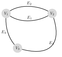
Figure 11: Modified splitcircle.

Therefore we consider a modified split circle network as depicted in Figure 11. In all the nodes the coupling conditions for a storage tank with $A_{m}=1$ are applied. As initial conditions we choose the constant water levels With the following initial data:

$$h^{1}(x,0) =h^{2}(x,0)=h^{4}(x,0)=5\ , h^{3}(x,0) =6$$

and $q^{i}(x,0)\equiv 0$ $i=1,\dots,4$. Using this setup instead of reusing the normal split circle with Riemann initial data ensures a clean Riemann problem at the junction without the interference of intermediary states.

The evolution of the states in the ODE of vertex $V_{1}$ is depicted in figure Figure 12. When zooming in, we can see that the $6$-th order scheme on the coarse grid of $50$ cells is closer to the reference solution computed on a grid of $200$ cells compared to the first order scheme. Even though the initial data is non smooth, which reduces the order of convergence to one, the solution benefits from the high order treatment.

In Figure 13 the solutions along edges $E_{1}$ and $E_{2}$ are shown. We observe that the shock emerging from the vertex profits greatly in sharpness from a higher order scheme as well. At $t=4$ the shock emerging from $V_{2}$ into $E_{4}$ after passing through $E_{1}$ and $E_{2}$ is shown in Figure 14. Again the solution of the $6$-th order scheme is much better than its first order counterpart.

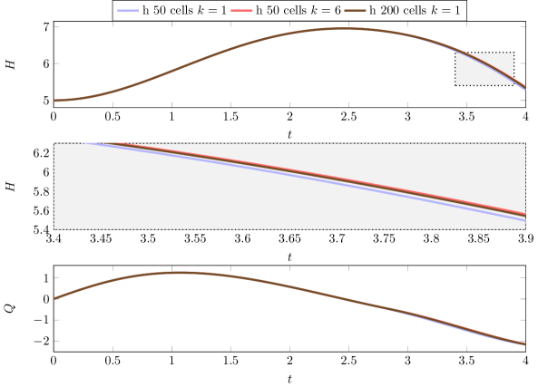
Figure 12: Schock investigation 7.4: Solution of the ODE in $V_{1}$ over time.

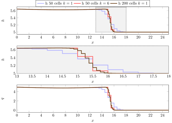
Figure 13: Schock investigation 7.4: Solution of the PDE on $E_{1}$/$E_{2}$ at $t=2$.

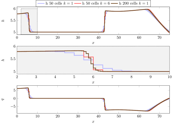
Figure 14: Schock investigation 7.4: Solution of the PDE on $E_{4}$ at $t=4$.

7.5 Shocks and lumped parameter models

In this test we consider a larger network of $32$ edges and $24$ nodes.

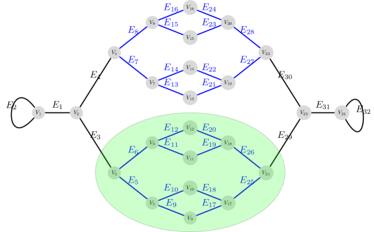
Figure 15: Split and join network with lumping of the green area.

As shown in Figure 15, the network is of a tree like structure, inspired by the human circulatory system e.g. [9]. The first four edges $E_{1},E_{2},E_{3},E_{4}$ and the last four $E_{29},E_{30},E_{31},E_{32}$ have a length of $L=25$, for all remaining edges we choose $L=2.5$. In the nodes equal height coupling conditions (22) are used. In order to investigate the influence of parameter lumping on the solution we model the lower half of the network by an ODE as described in Section 6.

As initial conditions we choose water at rest on all edges. On $E_{1}$ we impose the following Riemann Problem

$$h^{1}(0,x) =\begin{cases}3&x<18.5\\ 2&\text{else}\end{cases} q^{1}(0,x) =0\ ,$$

whereas the remaining edges continue these constant states

$$u^{2}(0,x) \equiv(3,0)^{T}\ , u^{i}(0,x) \equiv(2,0)^{T}\quad\forall i\geq 3\ .$$

Due to the symmetric nature of this setting and without applying the lumping to the lower part of the network, the solution in some branches of the network coincide . In this case we have the following identities

$$u^{3} =u^{4}\ ,$$

$$u^{5}=u^{6} =u^{7}=u^{8}\ ,$$

$$u^{9}=u^{10}=u^{11}=u^{12} =u^{13}=u^{14}=u^{15}=u^{16}\ ,$$

$$u^{17}=u^{18}=u^{19}=u^{20} =u^{21}=u^{22}=u^{23}=u^{24}\ ,$$

$$u^{25}=u^{26} =u^{27}=u^{28}\ ,$$

$$u^{29} =u^{30}\ .$$

Therefore it suffices to look at one edge of each group and we can directly compare the solutions of the lumped part of the network to its PDE counterparts.

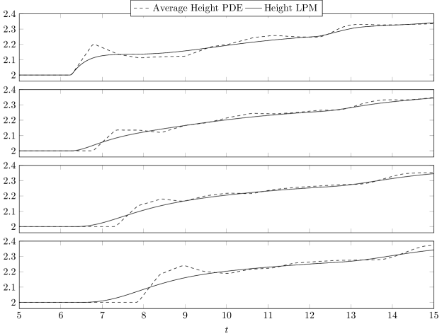
Figure 16: Shocks and LPM 7.5: Height components of the LPM model over time compared to the averaged solution of the full PDE simulation. From top to bottom: $E_{8}$, $E_{16}$, $E_{24}$ and $E_{28}$.

Figure 17: Shocks and LPM 7.5: Impulse components of the LPM model over time compared to the averaged solution of the full PDE simulation. From top to bottom: $E_{8}$, $E_{16}$, $E_{24}$ and $E_{28}$.

In Figure 16 we show the heights $H$ in the LPM vertex and the averaged heights on a corresponding edge located on the upper half of the network. Analogously the momentum components can be seen in Figure 17.

Due to the very coarse spatial resolution the states of the LPM model can not resolve the incoming shock wave accurately. Despite this strong diffusion caused by the model, the ODE captures the general behavior of the flow.

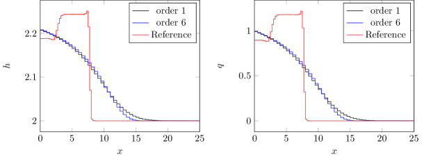
Figure 18: Shocks and LPM 7.5: Solution on $E_{29}$ after the LPM vertex compared to the reference solution on $E_{30}$.

The correct capturing of the wave speed can be observed in Figure 18. Here the solution on the edges $E_{29}$ and $E_{30}$ are shown. This provides a comparison between the shock wave, that has passed the lumped branch of the network and wave transported by the PDE model. Clearly the solution of the PDE model can resolve much finer structures.

7.5.1 Sources in Lumped Parameter Models

To demonstrate the necessity of hydrostatic reconstruction in LPM models, we simulate the following initial value problem consisting of shallow water equations on a split circle network with bottom elevation. $E_{2}$ and the two vertices are turned into a LPM. We use bottom profiles of linear, polynomial and trigonometrical type:

$$b_{1}(x) =0.3\frac{x}{25} b_{2}(x) =0.3\left(\frac{x}{25}+\left(\frac{x}{25}-\frac{1}{2}\right)^{2}-\frac{1}{4}\right) b_{3}(x) =0.3\left(\frac{x}{25}+\sin(\pi\frac{x}{25})\right)$$

$$H_{1}(x) =3+\mathbf{1}_{[\frac{1}{4}25,\frac{3}{4}25]}(x) H_{2}(x) \equiv 3 H_{3}(x) \equiv 3$$

$$\rho_{1}(x) =H_{1}(x)-b_{1}(x) \rho_{2}(x) =H_{2}(x)-b_{2}(x) \rho_{3}(x) =H_{3}(x)-b_{3}(x)$$

The results of the simulations are shown in figure 19 and 20. The solutions on the PDE edges are shown at $t=0.3$, the state of the ODE over the complete time interval. In the interior of the domain we can observe the asymptotically well balancedness of ADER schemes as reported in [20], the slightly stronger oscillations at the vertices are caused by the higher sensitivity of the coupling conditions amplifying the unavoidable errors stemming from the one sided polynomial reconstruction. The big oscillations however are avoided as expected.

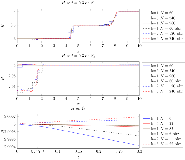
Figure 19: Well balanced LPM 7.5.1: $H$ on $E_{1}$.

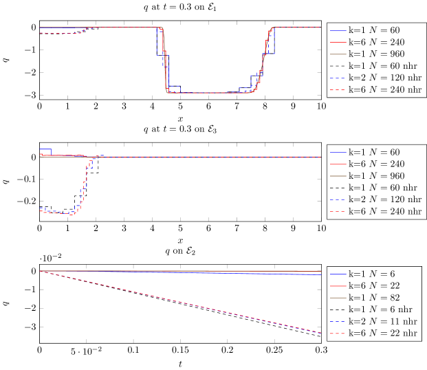
Figure 20: Well balanced LPM 7.5.1: $q$ on $E_{1}$.

8 Conclusion

High order GRP solvers for ODE vertices and LPM models of Toro-Castro and Harten, Enquist, Osher, Chakravarthy type are introduced in this work. Extensive tests showed that they indeed exhibit the high order of convergence they were designed for. Numerical examples showed that these technique can indeed be used to build very accurate and stable numerical methods for networks of conservation laws including vertices with ODEs and lumped parameter models. Especially the solver of Harten, Enquist, Osher, Chakravarthy type is a vast improvement in terms of applicability over the Toro-Castro approach introduced in [19].

References

- [1] M. Herty, M. Seaïd, Assessment of coupling conditions in water way intersections, International Journal for Numerical Methods in Fluids.
- [2] R. Borsche, A. Klar, Flooding in urban drainage systems: coupling hyperbolic conservation laws for sewer systems and surface flow, Internat. J. Numer. Methods Fluids 76 (11) (2014) 789–810.
- [3] R. Borsche, R. M. Colombo, M. Garavello, On the coupling of systems of hyperbolic conservation laws with ordinary differential equations, Nonlinearity 23 (11) (2010) 2749–2770.
- [4] P. Bales, O. Kolb, J. Lang, Hierarchical modelling and model adaptivity for gas flow on networks, in: G. Allen, J. Nabrzyski, E. Seidel, G. van Albada, J. Dongarra, P. Sloot (Eds.), Computational Science – ICCS 2009, Vol. 5544 of Lecture Notes in Computer Science, Springer Berlin Heidelberg, 2009, pp. 337–346.
- [5] J. Brouwer, I. Gasser, M. Herty, Gas Pipeline Models Revisited: Model Hierarchies, Nonisothermal Models, and Simulations of Networks, Multiscale Modeling & Simulation 9 (2) (2011) 601–623.
- [6] G. A. Reigstad, T. Flåtten, N. Erland Haugen, T. Ytrehus, Coupling constants and the generalized Riemann problem for isothermal junction flow, J. Hyperbolic Differ. Equ. 12 (1) (2015) 37–59.
- [7] G. M. Coclite, M. Garavello, B. Piccoli, Traffic flow on a road network, SIAM journal on mathematical analysis 36 (6) (2005) 1862–1886.
- [8] R. Borsche, A. Klar, S. Kühn, A. Meurer, Coupling traffic flow networks to pedestrian motion, Math. Models Methods Appl. Sci. 24 (2) (2014) 359–380.
- [9] L. O. Müller, E. F. Toro, A global multiscale mathematical model for the human circulation with emphasis on the venous system, International journal for numerical methods in biomedical engineering.
- [10] M. Á. Fernández, V. Milišić, A. Quarteroni, Analysis of a geometrical multiscale blood flow model based on the coupling of ODEs and hyperbolic PDEs, Multiscale Model. Simul. 4 (1) (2005) 215–236 (electronic).
- [11] V. Milišić, A. Quarteroni, Analysis of lumped parameter models for blood flow simulations and their relation with 1D models, M2AN Math. Model. Numer. Anal. 38 (4) (2004) 613–632.
- [12] G. Bretti, R. Natalini, M. Ribot, A hyperbolic model of chemotaxis on a network: a numerical study, ESAIM: Mathematical Modelling and Numerical Analysis 48 (2014) 231–258.
- [13] M. Herty, A. Klar, B. Piccoli, Existence of solutions for supply chain models based on partial differential equations, SIAM J. Math. Anal. 39 (1) (2007) 160–173.
- [14] L. O. Müller, E. F. Toro, A global multiscale mathematical model for the human circulation with emphasis on the venous system, International Journal for Numerical Methods in Biomedical Engineering 30 (7) (2014) 681–725.
- [15] E. F. Toro, Riemann solvers and numerical methods for fluid dynamics: a practical introduction, Springer, 2009.
- [16] R. J. LeVeque, Finite volume methods for hyperbolic problems, Cambridge University Press, Cambridge; New York, 2002.
- [17] G.-S. JIANG, C.-W. SHU, Efficient implementation of weighted eno schemes, JOURNAL OF COMPUTATIONAL PHYSICS 126 (1996) 202–228.
- [18] J. S. Hesthaven, T. Warburton, Nodal discontinuous Galerkin methods: algorithms, analysis, and applications, no. 54 in Texts in applied mathematics, Springer, New York, 2008.
- [19] R. Borsche, J. Kall, Ader schemes and high order coupling on networks of hyperbolic conservation laws, Journal of Computational Physics.
- [20] C. Castro, E. Toro, Solvers for the high-order riemann problem for hyperbolic balance laws, Journal of Computational Physics 227 (4) (2008) 2481–2513.
- [21] R. M. Colombo, G. Guerra, M. Herty, V. Schleper, Optimal control in networks of pipes and canals, SIAM Journal on Control and Optimization 48 (3) (2009) 2032–2050.
- [22] P. Domschke, O. Kolb, J. Lang, Adjoint-based error control for the simulation and optimization of gas and water supply networks, Appl. Math. Comput. 259 (2015) 1003–1018.
- [23] P. Degond, S. Göttlich, M. Herty, A. Klar, A network model for supply chains with multiple policies, Multiscale Model. Simul. 6 (3) (2007) 820–837.
- [24] S. Göttlich, A. Klar, Modeling and optimization of scalar flows on networks, in: Modelling and optimisation of flows on networks, Vol. 2062 of Lecture Notes in Math., Springer, Heidelberg, 2013, pp. 395–461.
- [25] R. Borsche, R. M. Colombo, M. Garavello, Mixed systems: Odes–balance laws, Journal of Differential Equations.
- [26] R. M. Colombo, M. Garavello, On the cauchy problem for the p-system at a junction, SIAM Journal on Mathematical Analysis 39 (5) (2008) 1456–1471.
- [27] S. Tan, C.-W. Shu, Inverse lax-wendroff procedure for numerical boundary conditions of conservation laws, Journal of Computational Physics 229 (21) (2010) 8144–8166.
- [28] E. Hairer, G. Wanner, Solving ordinary differential equations. II, Vol. 14 of Springer Series in Computational Mathematics, Springer-Verlag, Berlin, 2010, stiff and differential-algebraic problems, Second revised edition, paperback.
- [29] A. Bermudez, M. E. Vazquez, Upwind methods for hyperbolic conservation laws with source terms, Computers & Fluids 23 (8) (1994) 1049 – 1071.
- [30] E. Audusse, F. Bouchut, M.-O. Bristeau, R. Klein, B. Perthame, A Fast and Stable Well-Balanced Scheme with Hydrostatic Reconstruction for Shallow Water Flows, SIAM Journal on Scientific Computing 25 (6) (2004) 2050–2065.
- [31] A. Canestrelli, A. Siviglia, M. Dumbser, E. F. Toro, Well-balanced high-order centred schemes for non-conservative hyperbolic systems. applications to shallow water equations with fixed and mobile bed, Advances in Water Resources 32 (6) (2009) 834 – 844.