Associativity of the operator product expansion

Abstract

We consider a recursive scheme for defining the coefficients in the operator product expansion (OPE) of an arbitrary number of composite operators in the context of perturbative, Euclidean quantum field theory in four dimensions. Our iterative scheme is consistent with previous definitions of OPE coefficients via the flow equation method, or methods based on Feynman diagrams. It allows us to prove that a strong version of the “associativity” condition holds for the OPE to arbitrary orders in perturbation theory. Such a condition was previously proposed in an axiomatic setting in [1] and has interesting conceptual consequences: 1) One can characterise perturbations of quantum field theories abstractly in a sort of “Hochschild-like” cohomology setting, 2) one can prove a “coherence theorem” analogous to that in an ordinary algebra: The OPE coefficients for a product of two composite operators uniquely determine those for $n$ composite operators. We concretely prove our main results for the Euclidean $\varphi^{4}_{4}$ quantum field theory, covering also the massless case. Our methods are rather general, however, and would also apply to other, more involved, theories such as Yang-Mills theories.

1 Introduction

There exist many different approaches to quantum field theory. Many of these attempt to isolate within quantum field theory a kind of algebraic skeleton, which, in a sense depending on the particular framework, defines the theory and dictates its properties. The earliest manifestation of this kind of framework is that of local quantum physics due to Haag and Kastler [2] which is based on nets of local algebras of operators. A framework to isolate the algebraic core of many 2-dimensional conformal field theories is the theory of vertex operator algebras [3, 4]. The main idea of this framework is to formalise the properties of the operator product expansion (OPE) in such theories in order to build an algebraic structure capable of describing many interesting models in two dimensions.

Since the OPE ought to exist in any local quantum field theory in any dimension [5], it seems reasonable to define a quantum field theory by it, or more precisely, to attempt to build a self-consistent algebraic structure out of the OPE that can define a quantum field theory. The OPE is the statement that given a complete set of local operators ${\mathcal{O}}_{A_{i}}$, and given any sufficiently well-behaved quantum state $\Psi$, one has

$$\langle{\mathcal{O}}_{A_{1}}(x_{1})\cdots{\mathcal{O}}_{A_{N}}(x_{N})\rangle_{\Psi}\sim\sum_{B}\mathcal{C}_{A_{1}\ldots A_{N}}^{B}(x_{1},\ldots,x_{N})\ \langle{\mathcal{O}}_{B}(x_{N})\rangle_{\Psi}\,.$$ (1.1)

Here, $\mathcal{C}_{A_{1}\ldots A_{N}}^{B}$ are functions (or rather distributions), called OPE coefficients, and the symbol $``\sim"$ indicates that the relation is expected to hold asymptotically at short distances, in the sense that the difference between the left and right hand side of (1.1) vanishes if $x_{i}\to x_{N}$ for all $i\leq N$. In models of perturbative quantum field theory, such as the Euclidean $\varphi_{4}^{4}$-theory, the OPE was found to be not only asymptotic, but even convergent, in the sense that the sum over $B$ in (1.1) converges even for any finite separation of $x_{1},\ldots,x_{N}$ [6, 7].

These results strongly suggest that it should indeed be possible to view the OPE coefficients as defining the algebraic skeleton of the theory, and the 1-point functions $\langle{\mathcal{O}}_{B}(x_{N})\rangle_{\Psi}$ as carrying all the information about the state. The theory, then, should be defined by the OPE coefficients, whereas specific physical setups should be described by the collection of all 1-point functions, much in the way as a classical field theory is defined by a partial differential equation, and specific physical setups are described by boundary- or initial conditions for determining a given solution. (As an aside, let us point out that this viewpoint is, in fact, not only remarkably close to standard applications of the OPE in deep inelastic scattering, but also very attractive in curved spacetimes [8, 9], because it is much less clear there what physically preferred states would be in general.)

Of course, in order to define a concrete field theory, one must have a way to determine the OPE coefficients in the first place. The traditional way in Lagrangian field theory is to go back to correlation functions and proceed e.g. by the well-known (perturbative) methods described in [10, 11]. This is not really satisfactory if one wants, as we do, to view the OPE coefficients as the primary objects defining the theory, and not Lagrangians or correlation functions. In order to get around this, one clearly needs extra information on the OPE coefficients. One central property (formalised e.g. in the setting [1]) is a kind of associativity (also called “factorisation" or “consistency") condition, which can be motivated heuristically as follows: Consider an operator product ${\mathcal{O}}_{A_{1}}(x_{1}){\mathcal{O}}_{A_{2}}(x_{2}){\mathcal{O}}_{A_{3}}(x_{3})$, where $x_{i}\in\mathbb{R}^{4}$, and assume that $x_{2}$ is closer to $x_{1}$ than to $x_{3}$, i.e.

$$0<\frac{|x_{1}-x_{2}|}{|x_{2}-x_{3}|}\,<1\,.$$ (1.2)

Since the OPE is by its very nature a short distance expansion, one may hope to be able to perform the OPE of only the product ${\mathcal{O}}_{A_{1}}(x_{1}){\mathcal{O}}_{A_{2}}(x_{2})$ around the point $x_{2}$ first, leaving ${\mathcal{O}}_{A_{3}}(x_{3})$ as a “spectator". Such an expansion would have the form

$$\begin{split}\langle{\mathcal{O}}_{A_{1}}(x_{1}){\mathcal{O}}_{A_{2}}(x_{2}){\mathcal{O}}_{A_{3}}(x_{3})\rangle&\sim\sum_{B}\mathcal{C}_{A_{1}A_{2}}^{B}(x_{1},x_{2})\langle{\mathcal{O}}_{B}(x_{2}){\mathcal{O}}_{A_{3}}(x_{3})\rangle\\ &\sim\sum_{B,C}\mathcal{C}_{A_{1}A_{2}}^{B}(x_{1},x_{2})\,\mathcal{C}_{BA_{3}}^{C}(x_{2},x_{3})\langle{\mathcal{O}}_{C}(x_{3})\rangle\,,\end{split}$$ (1.3)

where we performed a second OPE in the second line. Comparison with eq.(1.1) yields an associativity condition

$$\mathcal{C}_{A_{1}A_{2}A_{3}}^{B}(x_{1},x_{2},x_{3})=\sum_{C}\mathcal{C}_{A_{1}A_{2}}^{C}(x_{1},x_{2})\,\mathcal{C}_{CA_{3}}^{B}(x_{2},x_{3})\,.$$ (1.4)

This condition puts strong restrictions on the OPE coefficients of the theory. To see this, assume also that

$$0<\frac{|x_{2}-x_{3}|}{|x_{1}-x_{3}|}\,<1\,.$$ (1.5)

We can repeat the argument above and arrive at the relation

$$\mathcal{C}_{A_{1}A_{2}A_{3}}^{B}(x_{1},x_{2},x_{3})=\sum_{C}\mathcal{C}_{A_{2}A_{3}}^{C}(x_{2},x_{3})\,\mathcal{C}_{A_{1}C}^{B}(x_{1},x_{3})\,.$$ (1.6)

The requirement of consistency of the alternative expansion schemes (1.4) and (1.6) on the domain $0<|x_{1}-x_{2}|<|x_{2}-x_{3}|<|x_{1}-x_{3}|$ yields

$$\sum_{C}\mathcal{C}_{A_{1}A_{2}}^{C}(x_{1},x_{2})\,\mathcal{C}_{CA_{3}}^{B}(x_{2},x_{3})=\sum_{C}\mathcal{C}_{A_{2}A_{3}}^{C}(x_{2},x_{3})\,\mathcal{C}_{A_{1}C}^{B}(x_{1},x_{3})\,,$$ (1.7)

which encodes highly non-trivial relations between the OPE coefficients. It was shown in [1] that these have various consequences:

• Multipoint OPE coefficients $\mathcal{C}_{A_{1}\ldots A_{N}}^{B}$ are uniquely determined in terms of the two-point coefficients $\mathcal{C}_{A_{1}A_{2}}^{B}$.

• Deformations (=perturbations) of OPE coefficients can be characterised as a cohomology of Hochschild type.

• OPE coefficients can be viewed as a (non-conformal, higher dimensional) version of vertex operator algebras.

The formal “derivation" of the associativity condition presented above is, of course, far from rigorous: For one thing, we have introduced the OPE as an asymptotic expansion, but in (1.2) and (1.5) we demanded finite separation of the points $x_{1},x_{2},x_{3}$. Furthermore, it is not obvious in what sense, if at all, the partial OPE performed in (1.3) holds. Lastly, we have implicitly exchanged the order of two infinite series in the step from (1.3) to (1.4) without any justification. Nevertheless, it is possible to see in some non-trivial examples of field theories such as in the massless Thirring model [12], or in the context of 2 dimensional conformal field theories [13] that the strong form of the associativity condition (1.7) in fact holds. Unfortunately, the arguments presented in these works are very specific to the peculiar properties of such models, giving no hint whatsoever what the situation might be e.g. for perturbatively defined models in Lagrangian field theory.

In the present paper we show that associativity of the OPE indeed holds to all orders in the perturbative Euclidean $\varphi_{4}^{4}$-theory. In fact, we even prove a generalisation of eq.(1.4) to more than three fields:

Theorem 1.

Denote by $[A]$ the dimension of the composite field ${\mathcal{O}}_{A}$. At any perturbation order $r\in\mathbb{N}$ in Euclidean $\varphi_{4}^{4}$-theory, there exist constants $c,K>0$ such that

$$\begin{split}\Big{|}\mathcal{C}_{A_{1}\ldots A_{N}}^{B}(x_{1},\ldots,x_{N})&-\sum_{[C]\leq D}\mathcal{C}_{A_{1}\ldots A_{M}}^{C}(x_{1},\ldots,x_{M})\,\mathcal{C}_{CA_{M+1}\ldots A_{N}}^{B}(x_{M},x_{M+1},\ldots,x_{N})\Big{|}_{r\text{-th order}}\\ &\leq K\cdot\xi^{\frac{D+1}{2}}\cdot\left(\frac{D+2}{\sqrt{\xi}-{\xi}}\right)^{c\cdot(\sum_{i}[A_{i}]+[B])}\cdot\frac{\max\limits_{1\leq i\leq N}(\frac{1}{m},|x_{i}-x_{N}|)^{[B]+1}}{\min\limits_{1\leq i<j\leq N}|x_{i}-x_{j}|^{\sum_{j}[A_{j}]+1}}\end{split}$$ (1.8)

holds for any $x_{1},\ldots,x_{N}$ such that

$$\xi:=\frac{\max_{1\leq i\leq M}|x_{i}-x_{M}|}{\min_{M<j\leq N}|x_{j}-x_{M}|}<1\,,$$ (1.9)

where $c=c(r)$ and $K=K(r,A_{1},\ldots,A_{N},B)$ do not depend on $D$. Since the r.h.s. of (1.8) vanishes in the limit $D\to\infty$, the bound implies that the associativity property

$$\mathcal{C}_{A_{1}\ldots A_{N}}^{B}(x_{1},\ldots,x_{N})=\sum_{[C]\leq D}\mathcal{C}_{A_{1}\ldots A_{M}}^{C}(x_{1},\ldots,x_{M})\,\mathcal{C}_{CA_{M+1}\ldots A_{N}}^{B}(x_{M},\ldots,x_{N})$$ (1.10)

holds up to any perturbation order on the domain defined by (1.9).

Remark:

A much weaker version of associativity was previously derived in [14]. There, it was shown that eq.(1.10) indeed holds up to any perturbation order, but only on the smaller domain

$$0<\frac{\max_{1\leq i\leq M}|x_{i}-x_{M}|}{\min_{j>M}|x_{j}-x_{M}|}<\varepsilon$$ (1.11)

for some constant $0<\varepsilon\ll 1$ which moreover decreases with the perturbation order. The weaker version is not suited in order to derive (1.7). Furthermore, the weaker version gives the misleading impression that associativity breaks down altogether beyond perturbation theory.

This result suggests that a quantum field theory can be defined by a set of OPE coefficients satisfying (1.10) on the domain (1.9), together with other simple straightforward, and reasonable requirements, see section 2 (for more details see [1] and also [15, 16] for curved spacetimes).

Even though, thanks to the above theorem, we may now feel much more confident that this viewpoint on QFT is correct, it does not tell us how to actually find QFTs, i.e., how to find actual solutions to the consistency requirements (1.10). Here a further independent idea is needed. This idea is to investigate how, given one solution to the consistency relations (e.g. the Gaussian free field), one can deform this solution to another one. As we recall below, one can nicely formulate an abstract deformation (=perturbation) theory of the algebraic structure based on (1.10) wherein perturbations are characterised as elements of some Hochschild type cohomology ring. However, this still does not give a good practical way of actually finding perturbations (to all orders in some small parameter, or even finite ones). Instead, we are going to rely on a recently found recursion formula for perturbative OPE coefficients [17]. This recursion formula is derived from the differential equation (a caret $\hat{\cdot}$ denotes omission)

$$\begin{split}&\partial_{g}\,\mathcal{C}_{A_{1}\ldots A_{N}}^{B}(x_{1},\ldots,x_{N})=-\int{\rm d}^{4}y\,\Big{[}\mathcal{C}_{{\mathfrak{L}}A_{1}\ldots A_{N}}^{B}(y,x_{1},\ldots,x_{N})\\ &-\sum_{i=1}^{N}\sum_{[D]\leq[A_{i}]}\!\!\!\mathcal{C}_{{\mathfrak{L}}A_{i}}^{D}(y,x_{i})\mathcal{C}_{A_{1}\ldots\widehat{A_{i}}D\ldots A_{N}}^{B}(x_{1},\ldots,x_{N})-\!\!\!\!\sum_{[D]<[B]}\!\!\mathcal{C}_{A_{1}\ldots A_{N}}^{D}(x_{1},\ldots,x_{N})\mathcal{C}_{{\mathfrak{L}}D}^{B}(y,x_{N})\Big{]}\,,\end{split}$$ (1.12)

for the change of an OPE coefficient if we change the action of the theory by a term of the form $g{\mathcal{O}}_{{\mathfrak{L}}}$ (where $g{\mathcal{O}}_{{\mathfrak{L}}}$ would be $g\varphi^{4}$ in our model). It is this relation, together with the well-known formulae for the OPE coefficients of the free theory ($g=0$), which is used in this paper to construct the coefficients of the interacting theory order by order in $g$, and to prove theorem 1. The bottom line is that this recursion formula (or the differential equation), together with the consistency relation (1.10) completely determine the OPE coefficients of a theory – hence the theory itself – and that these conditions are mutually consistent with each other.

This paper is organised as follows: We put our results into the context of axiomatic approaches in section 2. Section 3 contains the main results of the paper, which are then proved for the case of massive fields in section 4. The generalisation of the proof to massless fields can be found in section 5, followed by our conclusions in section 6. Some technical estimates are moved to an appendix.

2 General framework for QFT and remarks

Before delving into the derivation of the main results of this paper, we would like to explain the wider context provided by a specific proposal for the structure of QFT [1].

OPE algebras:

This framework is intended to formalise the properties of the OPE. In order to avoid writing many indices, one associates local fields $O_{A}$ in the theory with vectors $|v_{A}\rangle$ in some abstract vector space called $V$. The space $V$ is assumed to be graded in various ways which reflect the possibility to classify the different composite quantum fields in the theory by their spin, dimension, Bose/Fermi character, dimension etc. Thus, for example, if $V_{D}$ is the space of all fields of a fixed dimension $D$, then

$$V=\bigoplus_{D}V_{D}\,.$$ (2.13)

The infinite sum in this decomposition is understood without any closure taken. In other words, a vector $|v\rangle$ in $V$ has only non-zero components in a finite number of the direct summands in the decomposition (2.13). Typically the set of possible $D$-values is discrete and each $\dim V_{D}<\infty$.

On the vector space $V$, we assume the existence of an anti-linear, involutive operation called $\star:V\to V$ which should be thought of as taking the hermitian adjoint of the quantum fields. We also assume the existence of a linear grading map $\gamma:V\to V$ with the property $\gamma^{2}=id$. The vectors corresponding to eigenvalue $+1$ are to be thought of as "bosonic", while those corresponding to eigenvalue $-1$ are to be thought of as "fermionic".

So far, we have only defined a list of objects—in fact a linear space—that we think of as labelling the various composite quantum fields of the theory. The dynamical content and quantum nature of the given theory is next incorporated in the OPE associated with the quantum fields. This is a hierarchy denoted

$$\mathcal{C}=\bigg{(}\mathcal{C}(-,-),\mathcal{C}(-,-,-),\mathcal{C}(-,-,-,-),\dots\bigg{)}\,,$$ (2.14)

where each $(x_{1},\dots,x_{N})\mapsto\mathcal{C}(x_{1},\dots,x_{N})$ is a function on the "configuration space"

$$M_{N}:=\{(x_{1},\dots,x_{N})\in({\mathbb{R}}^{4})^{N}\mid x_{i}\neq x_{j}\quad\text{for all $1\leq i<j\leq N$}\}\,,$$ (2.15)

taking values in the linear maps

$$\mathcal{C}(x_{1},\dots,x_{N}):V\otimes\cdots\otimes V\to V\,,$$ (2.16)

where there are $N$ tensor factors of $V$. (The range of $\mathcal{C}(x_{1},\dots,x_{N})$ is actually in the closure $V^{**}$ of $V$ but we do not distinguish this in our notation.) The components of these maps in a basis of $V$ correspond to the OPE coefficients mentioned in the previous section. For one point, we set $\mathcal{C}(x_{1})=id:V\to V$, where $id$ is the identity map.

In order to have any chance of imposing stringent consistency conditions of the nature described in section 1, the maps $\mathcal{C}(-,\dots,-)$ must be real analytic functions on $M_{N}$, in the sense that their components $\mathcal{C}_{A_{1}\ldots A_{N}}^{B}(x_{1},\ldots,x_{N}):=\langle v_{B}|\mathcal{C}(x_{1},\ldots,x_{N})|v_{A_{1}}\otimes\ldots\otimes v_{A_{N}}\rangle$ are ordinary real analytic functions on $M_{N}$ with values in ${\mathbb{C}}$. The basic properties of quantum field theory are then expressed as the following further conditions on the OPE coefficients:

C1) Hermitian conjugation:

Denoting by $\star:V\to V$ the anti-linear map given by the star operation, we have $[\star,\gamma]=0$ and

$$\overline{\mathcal{C}(x_{1},\dots,x_{N})}=\star\,\mathcal{C}(x_{1},\dots,x_{N})\,\star^{\otimes N}$$ (2.17)

where $\star^{\otimes N}:=\star\otimes\cdots\otimes\star$ is the $N$-fold tensor product of the map $\star$, and where $\bar{\cdot}$ denotes complex conjugation.

C2) Euclidean invariance:

For a suitable representation $R$ of ${\rm Spin}(4)$ on $V$ and $a\in{\mathbb{R}}^{4}$, $g\in{\rm Spin}(4)$, we require

$$\mathcal{C}(gx_{1}+a,\dots,gx_{N}+a)=R^{*}(g)\,\mathcal{C}(x_{1},\dots,x_{N})\,R(g)^{\otimes N}\,,$$ (2.18)

where $R(g)^{\otimes N}$ stands for the $N$-fold tensor product $R(g)\otimes\dots\otimes R(g)$.

C3) Bosonic nature:

The OPE-coefficients are themselves "bosonic" in the sense that

$$\mathcal{C}(x_{1},\dots,x_{N})=\gamma\,\mathcal{C}(x_{1},\dots,x_{N})\,\gamma^{\otimes N}$$ (2.19)

where $\gamma^{\otimes N}$ is again a shorthand for the $n$-fold tensor product $\gamma\otimes\dots\otimes\gamma$.

C4) (Anti-)symmetry:

Let $\tau_{i-1,i}=(i-1\,\,i)$ be the permutation exchanging the $(i-1)$-th and the $i$-th object, which we define to act on $V\otimes\dots\otimes V$ by exchanging the corresponding tensor factors. Then we have

$$\mathcal{C}(x_{1},\dots,x_{i-1},x_{i},\dots,x_{N})\,\tau_{i-1,i}=\mathcal{C}(x_{1},\dots,x_{i},x_{i-1},\dots,x_{N})\,(-1)^{F_{i-1}F_{i}}$$ (2.21)

$$F_{i}:=\frac{1}{2}\,id^{\otimes(i-1)}\otimes(id-\gamma)\otimes id^{\otimes(N-i)}\,.$$

for all $1<i<N$. Here, the last factor is designed so that bosonic fields have symmetric OPE coefficients, and fermionic fields have anti-symmetric OPE-coefficients. The last point $x_{N}$ and the $N$-th tensor factor in $V\otimes\dots\otimes V$ do not behave in the same way under permutations, and the formula has to be slightly altered. See [1, eq.(3.38)] for the corresponding formula.

C5) Scaling:

Let ${\rm dim}:V\to V$ be the “dimension counting operator”, defined to act by multiplication with $D\in{\mathbb{R}}_{+}$ in each of the subspaces $V_{D}$ in the decomposition (2.13) of $V$ or, put differently, $\dim|v_{A}\rangle=[A]\cdot|v_{A}\rangle$. Then we require that ${\bf 1}\in V$ is the unique element up to rescaling with dimension $\dim({\bf 1})=0$, and that $[\dim,\gamma]=0$.

Furthermore, we require that, for any $\delta>0$ and any $(x_{1},\ldots,x_{n})\in M_{n}$,

$$\lim_{\epsilon\downarrow 0}\epsilon^{[A_{1}]+\ldots+[A_{N}]-[B]+\delta}\,\mathcal{C}_{A_{1}\ldots A_{N}}^{B}(\epsilon x_{1},\ldots,\epsilon x_{N})=0\,.$$ (2.22)

C6) Identity element:

We postulate that there exists a unique element ${\bf 1}$ of $V$ of dimension $[{\bf 1}]=0$, with the properties ${\bf 1}^{\star}={\bf 1},\gamma({\bf 1})={\bf 1}$, such that

$$\mathcal{C}(x_{1},\dots,x_{N})|v_{1}\otimes\cdots{\bf 1}\otimes\cdots v_{N-1}\rangle=\mathcal{C}(x_{1},\dots\widehat{x_{i}},\dots x_{N})|v_{1}\otimes\cdots\otimes v_{N-1}\rangle\,.$$ (2.23)

where ${\bf 1}$ is in the $i$-th tensor position, with $i\leq N-1$. When ${\bf 1}$ is in the $N$-th tensor position, the analogous requirement takes a slightly more complicated form (see [1, chapter 3]).

C7) Factorisation:

$$\mathcal{C}(x_{1},\ldots,x_{N})=\mathcal{C}(x_{M},\ldots,x_{N})(\mathcal{C}(x_{1},\ldots,x_{M})\otimes id^{\otimes(N-M)})$$ (2.24)

on the domain

$$\frac{\max_{1\leq i\leq M}|x_{i}-x_{M}|}{\min_{M<j\leq N}|x_{j}-x_{M}|}<1\,.$$ (2.25)

Note that this condition is an “index free" restatement of (1.10), the main result of our paper in the context of perturbation theory.

Definition 1.

A quantum field theory is defined as a pair consisting of an infinite dimensional vector space $V$ with decomposition (2.13) and maps $\star,\gamma,\dim$ with the properties described above, together with a hierarchy of OPE coefficients $\mathcal{C}:=(\mathcal{C}(-,-),\mathcal{C}(-,-,-),\dots)$ satisfying properties C1)–C7).

It is natural to identify quantum field theories if they only differ by a redefinition of the fields. Informally, a field redefinition means that one changes ones definition of the quantum fields of the theory from ${\mathcal{O}}_{A}(x)$ to $\widehat{\mathcal{O}}_{A}(x)=\sum_{B}Z_{A}^{B}{\mathcal{O}}_{B}(x)$, where $Z_{A}^{B}$ is some matrix on field space. The OPE coefficients of the redefined fields differ from the original ones accordingly by factors of this matrix. We formalise this in the following definition:

Definition 2.

Let $(V,\mathcal{C})$ and $(\widehat{V},\widehat{\mathcal{C}})$ be two quantum field theories. If there exists an invertible linear map $Z:V\to\widehat{V}$ with the properties

$$Z\,R(g)=\hat{R}(g)\,Z\,,\quad Z\,\gamma=\hat{\gamma}\,Z\,,\quad Z\,\star=\hat{\star}\,Z\,,\quad Z({\bf 1})=\widehat{\bf 1}\,,\quad\widehat{\dim}\,Z\geq Z\,\dim\,,$$ (2.26)

together with

$$\mathcal{C}(x_{1},\dots,x_{N})=Z^{-1}\,\widehat{\mathcal{C}}(x_{1},\dots,x_{N})\,Z^{\otimes N}$$ (2.27)

for all $N$, where $Z^{\otimes N}=Z\otimes\dots\otimes Z$, then the two quantum field theories are said to be equivalent, and $Z$ is said to be a field redefinition.

The main result of our paper, Thm. 1, leads to the following conclusion:

Corollary 1.

The OPE in perturbative Euclidean $\varphi_{4}^{4}$-theory satisfies axioms C1)-C7) in the sense of formal perturbation series in $g$, i.e. at each fixed order in $g$.

Proof.

The symmetry requirements C1)-C4) and the identity axiom C6) are quite easily checked: They can be explicitly checked in the free theory, and one verifies directly that they are preserved by the recursion formula (1.12), which we use to define perturbative OPE coefficients. The scaling requirement C5) follows e.g. from the bounds proven in [17]. By far the most non-trivial challenge is to prove C7) (factorisation). This is the content of thm.1 of the present paper. ∎

Vertex algebras:

Another corollary of theorem 1 is that perturbation theory defines an analog of a vertex operator algebra: First, define vertex operators $Y(x,v):V\to V$ as the endomorphism of $V$ whose matrix elements are given by

$$\langle v_{C}|Y(x,v_{A})|v_{B}\rangle:=\mathcal{C}_{AB}^{C}(x,0)$$ (2.28)

for any $x\neq 0$. The relation (1.7), which is a consequence of our main theorem, may now be written as

$$Y(v,x)Y(w,y)=Y(Y(v,x-y)w,y)\,,$$ (2.29)

where the spacetime arguments are required to satisfy $|x|>|y|>|x-y|>0$ and where $v,w$ are elements of $V$. An almost identical quadratic relation first appeared in the study of conformal field theories in two dimensions, where it is one of the crucial properties (called “locality condition") of the vertex operator algebras [4]. It should be stressed, however, that in our context, where conformal symmetry is not required, the condition above is really a highly non-trivial statement on the convergence of the infinite sums implicit in eq.(2.29), whereas the same equality in the CFT context is understood in terms of formal power series.

Abstract perturbation theory:

The constraint imposed by the factorisation condition C5) at the three point level can be rewritten as

$$\begin{split}\mathcal{C}(x_{2},x_{3})\Big{(}\mathcal{C}(x_{1},x_{2})\otimes id\Big{)}&-\mathcal{C}(x_{1},x_{3})\Big{(}id\otimes\mathcal{C}(x_{2},x_{3})\Big{)}=0\\ &\text{ for }0<|x_{1}-x_{2}|<|x_{2}-x_{3}|<|x_{1}-x_{3}|,\end{split}$$ (2.30)

which is just an “index free" version of eq.(1.7). Although we will not use this in the present paper, all higher constraints can be derived from this one, see [1]. In the very abstract general framework of an OPE algebra, we may ask the question when it is possible to find a 1-parameter deformation $\mathcal{C}(x_{1},x_{2};g)$ of these coefficients by a parameter $g$ so that the associativity condition continues to hold, at least in the sense of formal power series in $g$. (Actually, the analogues of the symmetry condition (2.21), the scaling condition (2.22), the hermitian conjugation, the Euclidean invariance, and the unit axiom should hold as well for the perturbation. However, these conditions are much more trivial in nature than (2.30), because the conditions are linear in $\mathcal{C}(x_{1},x_{2})$. These conditions could therefore easily be included in our discussion, but would distract from the main point.)

One can show that such perturbations can be characterised in a cohomological framework. To set up this framework, we consider the non-empty, open domains of $({\mathbb{R}}^{4})^{N}$ defined by

$${\cal F}_{N}=\{(x_{1},\dots,x_{N})\in M_{N};\,\,\,r_{1\,i-1}<r_{i-1\,i}<r_{i-2\,i}<\dots<r_{1i},\,\,\,1<i\leq N\}\subset M_{N}\,,$$ (2.31)

where $r_{ij}:=|x_{i}-x_{j}|$. We define $\Omega^{N}(V)$ to be the set of all real analytic functions $f_{N}$ on the domain ${\cal F}_{N}$ that are valued in the linear maps

$$f_{N}(x_{1},\dots,x_{N}):V\otimes\dots\otimes V\to V,\quad(x_{1},\dots,x_{N})\in{\cal F}_{N}\,.$$ (2.32)

We next introduce a boundary operator $b:\Omega^{N}(V)\to\Omega^{N+1}(V)$ by the formula

$$(bf_{N})(x_{1},\dots,x_{N+1}):=\mathcal{C}_{0}(x_{1},x_{N+1})(id\otimes f_{N}(x_{2},\dots,x_{N+1}))$$ (2.33)

$$+\sum_{i=1}^{N}(-1)^{i}f_{N}(x_{1},\dots,\widehat{x}_{i},\dots,x_{N+1})(id^{\otimes(i-1)}\otimes\mathcal{C}_{0}(x_{i},x_{i+1})\otimes id^{\otimes(N-i)})$$

$$+(-1)^{N+1}\,\mathcal{C}_{0}(x_{N},x_{N+1})(f_{N}(x_{1},\dots,x_{N})\otimes id)\,.$$

Here $\mathcal{C}_{0}(x_{1},x_{2})$ is the OPE-coefficient of the undeformed theory defined by $g=0$, and a caret means omission. The definition of $b$ involves a composition of $\mathcal{C}_{0}$ with $f_{N}$, and hence, when expressed in a basis of $V$, implicitly involves an infinite summation over the basis elements of $V$. We must therefore assume here (and in similar formulas in the following) that these sums converge on the set of points $(x_{1},\dots,x_{N+1})$ in the domain ${\cal F}_{N+1}$. We shall then say that $bf_{N}$ exists, and we collect such $f_{N}$ in the domain of $b$,

$${\rm dom}(b)=\bigoplus_{N\geq 1}\{f_{N}\in\Omega^{N}(V)\mid\text{$bf_{N}$ exists and is in $\Omega^{N+1}(V)$}\}\,.$$ (2.34)

When we write $bf_{N}$, it is understood that $f_{N}\in\Omega^{N}(V)$ is in the domain of $b$. One can show:

Lemma 1.

The map $b$ is a differential, i.e., $b^{2}f_{N}=0$ for $f_{N}$ in the domain of $b$ such that $bf_{N}$ is also in the domain of $b$.

Let us define the kernel $Z^{N}(V,\mathcal{C})$ of $b$ on $\Omega^{N}(V)$ as the linear space of all $f_{N}\in\Omega^{N}(V)\cap{\rm dom}(b)$ such that $bf_{N}=0$. Similarly, define the range $B^{N}(V,\mathcal{C})$ in $\Omega^{N}(V)$ to be the linear space of all $f_{N}=bf_{N-1}$ such that $f_{N-1}\in\Omega^{N-1}(V)\cap{\rm dom}(b)$ and such that $f_{N}$ is in ${\rm dom}(b)$. By the above lemma, we can then define a cohomology ring associated with the differential $b$ as

$$H^{N}(V;\mathcal{C})=\frac{Z^{N}(V;\mathcal{C})}{B^{N}(V;\mathcal{C})}:=\frac{\{{\rm ker}\,b:\Omega^{N}(V)\to\Omega^{N+1}(V)\}\cap{\rm dom}(b)}{\{{\rm ran}\,b:\Omega^{N-1}(V)\to\Omega^{N}(V)\}\cap{\rm dom}(b)}\,.$$ (2.35)

As we will now see, the problem of finding a 1-parameter family of perturbations $\mathcal{C}(x_{1},x_{2};g)$ such that our associativity condition (2.30) continues to hold for $\mathcal{C}(x_{1},x_{2};g)$ to all orders in $g$ can be elegantly and compactly formulated in terms of this ring. If we let

$$\mathcal{C}_{i}(x_{1},x_{2})=\frac{1}{i!}\,\frac{d^{i}}{dg^{i}}\mathcal{C}(x_{1},x_{2};g)\Bigg{|}_{g=0}\,,$$ (2.36)

then we note that the first order associativity condition,

$$\mathcal{C}_{0}(x_{2},x_{3})\Big{(}\mathcal{C}_{1}(x_{1},x_{2})\otimes id\Big{)}-\mathcal{C}_{0}(x_{1},x_{3})\Big{(}id\otimes\mathcal{C}_{1}(x_{2},x_{3})\Big{)}+$$

$$\mathcal{C}_{1}(x_{2},x_{3})\Big{(}\mathcal{C}_{0}(x_{1},x_{2})\otimes id\Big{)}-\mathcal{C}_{1}(x_{1},x_{3})\Big{(}id\otimes\mathcal{C}_{0}(x_{2},x_{3})\Big{)}=0\,\,,$$ (2.37)

valid for $(x_{1},x_{2},x_{3})\in{\cal F}_{3}$, is equivalent to the statement that

$$b\mathcal{C}_{1}=0\,,$$ (2.38)

where here and in the following, $b$ is defined in terms of the unperturbed OPE-coefficient $\mathcal{C}_{0}$. Thus, $\mathcal{C}_{1}$ has to be an element of $Z^{2}(V;\mathcal{C}_{0})$. Let $Z(g):V\to V$ be a $g$-dependent field redefinition in the sense of defn. 2, and suppose that $\mathcal{C}(x_{1},x_{2})$ and $\mathcal{C}(x_{1},x_{2};g)$ are connected by the field redefinition. To first order, this means that

$$\mathcal{C}_{1}(x_{1},x_{2})=-Z_{1}\mathcal{C}_{0}(x_{1},x_{2})+\mathcal{C}_{0}(x_{1},x_{2})(Z_{1}\otimes id+id\otimes Z_{1})\,,$$ (2.39)

or equivalently, that $bZ_{1}=\mathcal{C}_{1}$, where $Z_{i}=\frac{1}{i!}\,\frac{d^{i}}{dg^{i}}Z(g)|_{g=0}$. Thus, the first order deformations of $\mathcal{C}_{0}$ modulo the trivial ones defined by eq. (2.39) are given by the classes in $H^{2}(V;\mathcal{C}_{0})$. The associativity condition for the $i$-th order perturbation (assuming that all perturbations up to order $i-1$ exist) can be written as the following condition for $(x_{1},x_{2},x_{3})\in{\cal F}_{3}$:

$$\mathcal{C}_{0}(x_{2},x_{3})\Big{(}\mathcal{C}_{j}(x_{1},x_{2})\otimes id\Big{)}-\mathcal{C}_{j}(x_{1},x_{3})\Big{(}id\otimes\mathcal{C}_{0}(x_{2},x_{3})\Big{)}+$$ (2.40)

$$\mathcal{C}_{j}(x_{2},x_{3})\Big{(}\mathcal{C}_{0}(x_{1},x_{2})\otimes id\Big{)}-\mathcal{C}_{0}(x_{1},x_{3})\Big{(}id\otimes\mathcal{C}_{j}(x_{2},x_{3})\Big{)}=w_{i}(x_{1},x_{2},x_{3})\,,$$

where $w_{i}\in\Omega^{3}(V)$ is defined by

$$w_{i}(x_{1},x_{2},x_{3}):=-\sum_{j=1}^{i-1}\mathcal{C}_{i-j}(x_{1},x_{3})(id\otimes\mathcal{C}_{j}(x_{2},x_{3}))-\mathcal{C}_{i-j}(x_{2},x_{3})(\mathcal{C}_{j}(x_{1},x_{2})\otimes id)\,.$$ (2.41)

We assume here that all infinite sums implicit in this expression converge on ${\cal F}_{3}$. This equation may be written alternatively as

$$b\mathcal{C}_{i}=w_{i}\,.$$ (2.42)

We would like to define the $i$-th order perturbation by solving this linear equation for $\mathcal{C}_{i}$. Clearly, a necessary condition for there to exist a solution is that $bw_{i}=0$ or $w_{i}\in Z^{3}(V,\mathcal{C}_{0})$, and this can indeed be shown to be the case. If a solution to eq. (2.42) exists, i.e. if $w_{i}\in B^{3}(V,\mathcal{C}_{0})$, then any other solution will differ from this one by a solution to the corresponding "homogeneous" equation. Trivial solutions to the homogeneous equation of the form $bZ_{i}$ again correspond to an $i$-th order field redefinition and are not to be counted as genuine perturbations. In summary, the perturbation series can be continued at $i$-th order if $[w_{i}]$ is the trivial class in $H^{3}(V;\mathcal{C}_{0})$, so $[w_{i}]$ represents a potential $i$-th order obstruction to continue the perturbation series. If there is no obstruction, then the space of non-trivial $i$-th order perturbations is given by $H^{2}(V;\mathcal{C}_{0})$. In particular, if we knew e.g. that $H^{2}(V;\mathcal{C}_{0})\neq 0$ while $H^{3}(V;\mathcal{C}_{0})=0$, then perturbations could be defined to arbitrary orders in $g$.

The relationship of this abstract framework with the results of the present paper is the following:

Corollary 2.

Let $\mathcal{C}_{0}$ be the OPE coefficients of a free, scalar Euclidean quantum field theory, and let $\mathcal{C}_{j},j>0$ be their perturbations, as defined by the recursion formula (1.12). Then

1. $\mathcal{C}_{1}$ is a non-trivial element of $H^{2}(V;\mathcal{C}_{0})$, and

2. all higher obstructions $[w_{i}]\in H^{3}(V;\mathcal{C}_{0})$ vanish.

Proof.

Non-triviality of $\mathcal{C}_{1}$ follows from the fact that the recursion formula (1.12) can not be written as a mere redefinition of the composite fields. The second point, i.e. vanishing of obstructions $[w_{i}]\in H^{3}(V;\mathcal{C}_{0})$, follows directly from the main result of the present paper, thm.1, because it is equivalent to associativity order-by-order in $g$. ∎

3 The Associativity Theorem

In the present section we are going to state our other main results, which will imply the bound stated in thm. 1 within perturbative Euclidean $\varphi^{4}$-theory in four dimensions with classical action

$$S=\int{\rm d}^{4}x\left(\frac{1}{2}(\partial\varphi)^{2}+\frac{m^{2}}{2}\varphi^{2}+\frac{g}{4!}\varphi^{4}\right)\,.$$ (3.43)

Throughout the present section we will restrict attention to the massive case $m^{2}>0$. The generalisation of our proof to massless fields is discussed afterwards in section 5.

We write the composite operators of our model explicitly as

$${\mathcal{O}}_{A}=\partial^{\alpha_{1}}\varphi\cdots\partial^{\alpha_{n}}\varphi,\quad A=(\alpha_{1},\ldots,\alpha_{n}),\quad\alpha_{i}\in\mathbb{N}^{4}\,,$$ (3.44)

which means that the corresponding dimension of the field ${\mathcal{O}}_{A}$ is given by

$$[A]=\sum_{i=1}^{n}(1+|\alpha_{i}|)\,,\qquad\text{ where }|\alpha|=\sum_{\mu=1}^{4}|\alpha_{\mu}|\text{ for }\alpha\in\mathbb{N}^{4}\,.$$ (3.45)

Let us denote the (formal) perturbation series for OPE coefficients by

$$\mathcal{C}_{A_{1}\ldots A_{N}}^{B}(x_{1},\ldots,x_{N})=:\sum_{r=0}^{\infty}(\mathcal{C}_{r})_{A_{1}\ldots A_{N}}^{B}(x_{1},\ldots,x_{N})\cdot g^{r}\,,$$ (3.46)

where the perturbative OPE coefficients $(\mathcal{C}_{r})_{A_{1}\ldots A_{N}}^{B}$ are defined recursively through eq.(1.12). Further, denote by

$$\begin{split}&(R_{r}^{D})_{A_{1}\ldots A_{M};A_{M+1}\ldots A_{N}}^{B}(x_{1},\ldots,x_{N}):=\\ &(\mathcal{C}_{r})_{A_{1}\ldots A_{N}}^{B}(x_{1},\ldots,x_{N})-\sum_{s+t=r}\sum_{{[C]\leq D}}(\mathcal{C}_{s})_{A_{1}\ldots A_{M}}^{C}(x_{1},\ldots,x_{M})\,(\mathcal{C}_{t})_{CA_{M+1}\ldots A_{N}}^{B}(x_{M},\ldots,x_{N})\end{split}$$ (3.47)

the remainder of the associativity condition at $r$-th perturbation order and truncated at operators ${\mathcal{O}}_{C}$ of dimension $[C]=D$. Our strategy is to establish the bound (1.8) by an induction which is based on the recursion formula (1.12). In order to obtain the sharp bound (1.8), we will have to formulate our induction hypothesis not in terms of the remainder functions $(R_{r}^{D})_{A_{1}\ldots A_{M};A_{M+1}\ldots A_{N}}^{B}$, but in terms of much more general objects, containing multiple summations over products of OPE coefficients (see definition 4 below). These more general expressions are most conveniently organised in terms of decorated rooted trees. Before we can state our main inductive bound, we therefore have to introduce some additional notation.

First, we agree on a vocabulary for rooted trees $T$, which is summarised in the following glossary (cf. [18, chapter 3.2.2]):

Symbol	Definition
$\mathcal{V}(T)$	Vertices of the tree $T$.
$\mathcal{L}(T)$	Leaves of $T$, i.e. vertices of degree 1 (the degree of a vertex is the number of edges adjacent to it).
$\mathcal{R}(T)$	The root of $T$, $\mathcal{R}\in\mathcal{V}$.
$\mathcal{I}(T)$	Internal vertices of $T$, i.e. non-leaf vertices.
$\mathcal{I}_{\mathcal{R}}(T)$	Internal vertices of $T$ without the root, i.e. $\mathcal{I}_{\mathcal{R}}:=\mathcal{I}\setminus\mathcal{R}$ .
$\mathcal{B}(T)$	The set of branches of $T$. A branch $b\in\mathcal{B}$ is a path connecting a leaf to the root, where we use the convention that leaves and root are not part of the branch, i.e. $\mathcal{B}\subset\mathcal{I}_{\mathcal{R}}$.
$\operatorname{ch}(v)$	The children of a vertex $v\in\mathcal{V}$ are the vertices adjacent to $v$ which are further from the root.
$\operatorname{pa}(v)$	The parent of a vertex $v\in\mathcal{V}$ is the vertex adjacent to $v$ which is closer to the root.
$\operatorname{sb}(v)$	The siblings of a vertex $v\in\mathcal{V}$ are the children of the parent of $v$ not including $v$ itself, i.e. $\operatorname{sb}(v):=\operatorname{ch}(\operatorname{pa}(v))\setminus\{v\}$.
$\operatorname{de}(v)$	The descendents of a vertex $v\in\mathcal{V}$ are the vertices on the paths from $v$ to the leaves.
$\operatorname{an}(v)$	The ancestors of a vertex $v\in\mathcal{V}$ are the vertices on the path from $v$ to the root.

Next, we add decorations to these trees:

Definition 3 (Weighted trees).

Let $\vec{x}=(x_{1},\ldots,x_{N})\in\mathbb{R}^{4N}$ and $\vec{A}=(A_{1},\ldots,A_{n})$, where $A_{i}\in\mathbb{N}^{4n_{i}}$ are multi-indices and where $n\geq N$. We define $\mathcal{T}(\vec{x};\vec{A})$ to be the set of rooted trees $T$ with the following properties:

1. $T$ has $n$ vertices and $N$ leaves.

2. Vertices in $\mathcal{I}_{\mathcal{R}}$ have degree larger than $2$.

3. To each vertex $v\in\mathcal{V}(T)$ we associate a pair $(x_{v},A_{v})$ called the weight of $v$, where $x_{v}\in\mathbb{R}^{4}$ is a four-vector and $A_{v}\in\mathbb{N}^{4n_{v}}$ a multi index, such that

   • if $v\in\mathcal{I}(T)$, then $x_{v}\in\{x_{w}:w\in\operatorname{ch}(v)\}$, i.e. $x_{v}$ has to be equal to one of the four-vectors associated to the children of $v$. To the leaves $v\in\mathcal{L}(T)$ we associate bijectively the vectors $(x_{1},\ldots,x_{N})$, i.e. $(x_{v})_{v\in\mathcal{L}}=\vec{x}$.

   • $(A_{v})_{v\in\mathcal{V}(T)}=\vec{A}$, i.e. the mapping between multi-indices and vertices is one-to-one.

See fig.1 for an example of three such trees.

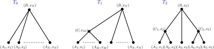
Figure 1: Example of weighted trees $T_{0}\in\mathcal{T}((A_{1},\ldots,A_{N},B);(x_{1},\ldots,x_{N}))$, $T_{1}\in\mathcal{T}((A_{1},\ldots,A_{N},B,C);(x_{1},\ldots,x_{N}))$ and $T_{2}\in\mathcal{T}((A_{1},\ldots,A_{5},B,C_{1},C_{2});(x_{1},\ldots,x_{5}))$.

With this notation in place, we can now give a compact definition of the objects appearing in our induction hypothesis:

Definition 4 (Contractions of OPE coefficients).

Given a tree $T\in\mathcal{T}(\vec{x};\vec{A})$, we define

$$({\mathcal{P}}_{r})(T):=\prod_{v\in\mathcal{I}(T)}\sum_{\sum\limits_{u\in\mathcal{I}(T)}r_{u}=r}(\mathcal{C}_{r_{v}})_{(A_{e})_{e\in\operatorname{ch}(v)}}^{A_{v}}((x_{e})_{e\in\operatorname{ch}(v)};x_{v})\,.$$ (3.48)

The argument behind the semicolon in the OPE coefficients specifies the reference point, i.e.

$$\mathcal{C}_{A_{1}\ldots A_{N}}^{B}(x_{1},\ldots,x_{N};x_{1})=\mathcal{C}_{A_{2}\ldots A_{N}A_{1}}^{B}(x_{2},\ldots,x_{N},x_{1})$$ (3.49)

for example.

Examples:

For the weighted trees depicted in fig.1, the definition yields

$$({\mathcal{P}}_{r})(T_{0}) =(\mathcal{C}_{r})_{A_{1}A_{2}\ldots A_{N}}^{B}(x_{1},x_{2},\ldots,x_{N})$$ (3.50)

$$({\mathcal{P}}_{r})(T_{1}) =\sum_{r_{1}+r_{2}=r}(\mathcal{C}_{r_{1}})_{A_{1}\ldots A_{M}}^{C}(x_{1},\ldots,x_{M})\ (\mathcal{C}_{r_{2}})_{CA_{M+1}\ldots A_{N}}^{B}(x_{M},\ldots,x_{N})$$ (3.51)

$$({\mathcal{P}}_{r})(T_{2}) =\sum_{r_{1}+r_{2}+r_{3}=r}(\mathcal{C}_{r_{1}})_{A_{1}A_{2}}^{C_{1}}(x_{1},x_{2})\ (\mathcal{C}_{r_{2}})_{A_{4}A_{5}}^{C_{2}}(x_{4},x_{5})\ (\mathcal{C}_{r_{3}})_{C_{1}A_{3}C_{2}}^{B}(x_{2},x_{3},x_{5})\,.$$ (3.52)

We are now ready to state our second main theorem, which directly implies theorem 1.

Theorem 2.

Up to any perturbation order $r\in\mathbb{N}$, OPE coefficients of massive Euclidean $\varphi_{4}^{4}$-theory satisfy the following two properties:

1. Given a tree $T\in\mathcal{T}(\vec{x};\vec{A})$ and given a collection of integers $(D_{i})_{i\in\mathcal{I}_{\mathcal{R}}}$, fix any branch $b\in\mathcal{B}(T)$ in the tree such that $x_{v}=x_{w}$ for all $v,w\in b(T)$ and define the shorthand $\mathfrak{D}_{T}:=\sum_{v\in\mathcal{L}\cup\mathcal{R}(T)}[A_{v}]$. For any choice of constants $\varepsilon\in(0,2^{-(\mathfrak{D}_{T}+4r+3)}]$ and $\delta_{v}\in(0,1)$, one has the bound

   $$\begin{split}\Big{|}\prod_{i\in\mathcal{I}_{\mathcal{R}}(T)}\sum_{[A_{i}]=D_{i}}({\mathcal{P}}_{r})(T)\Big{|}\leq&\ \frac{\max\limits_{i\in\operatorname{ch}(\mathcal{R})}|x_{i}-x_{\mathcal{R}}|^{[A_{\mathcal{R}}]}}{\prod\limits_{i\in\mathcal{L}}\min\limits_{j\in\operatorname{sb}(i)}|x_{i}-x_{j}|^{[A_{i}]}}\ \prod\limits_{i\in\mathcal{I}_{\mathcal{R}}}\xi_{i}^{D_{i}}\\ \times&\ K\ \bigg{(}\frac{(1+\varepsilon)^{\sum_{w\in b}[A_{w}]}}{\varepsilon^{\sum_{v\in\mathcal{V}\setminus b}[A_{v}]}}\cdot\prod_{w\in b}(D_{w}+1)^{\mathfrak{D}_{T}}\bigg{)}^{8^{r+1}}\\ \times&\prod\limits_{v\in\mathcal{I}}\left(\frac{\sup_{i\in\operatorname{ch}(v)}(|x_{i}-x_{v}|,1/m)}{m^{\theta(\Delta_{v})}\min\limits_{i\neq j\in\operatorname{ch}(v)}|x_{i}-x_{j}|^{1+\theta(\Delta_{v})}}\right)^{\delta_{v}}\end{split}$$ (3.53)

   where the constant $K>0$ depends neither on the integers $D_{i}$ nor on $\varepsilon$ or the $\delta_{v}$, where

   $$\xi_{i}(T):=\frac{\max_{e\in\operatorname{ch}(i)}|x_{e}-x_{i}|}{\min_{e\in\operatorname{sb}(i)}|x_{e}-x_{i}|}\,,$$ (3.54)

   where $\theta$ is the Heaviside step function and where $\Delta_{v}:=\sum_{e\in\operatorname{ch}(v)}[A_{e}]-[A_{v}]$.

2. For any $\xi<1$ one has

   $$\lim_{D\to\infty}(R_{r}^{D})_{A_{1}\ldots A_{M};A_{M+1}\ldots A_{N}}^{B}(x_{1},\ldots,x_{N})=0\,,$$ (3.55)

   where $\xi$ is defined as in eq.(1.11).

Remark:

Before we come to the proof of the theorem, let us take a moment to have a closer look at the result in order to get a better intuition for the complicated expression (3.53). The origin of the various terms in the bound (3.53) can be roughly understood as follows:

1. The first line reflects the behaviour one would expect from naive power counting if one assumes that an OPE coefficient behaves as $\mathcal{C}_{A_{1}\ldots A_{N}}^{B}(x_{1},\ldots,x_{N})\sim\max|x_{i}-x_{N}|^{[B]}/\prod_{i}\min|x_{i}-x_{j}|^{\sum[A_{i}]}$.

2. The second line captures all combinatorial factors, in particular those caused by the summations over multi indices $[C_{i}]=D_{i}$ associated to the internal vertices of the tree $T$ and those arising in perturbation theory. Note that only this second line depends on the perturbation order $r$.

3. In the last line, the factors including the Heaviside function are a relict of the exponential decay of the massive propagator. These factors are needed in the induction in order to avoid infrared divergences. Finally, the factor $(\sup_{i\in\operatorname{ch}(v)}(|x_{i}-x_{v}|,1/m)/\min\limits_{i\neq j\in\operatorname{ch}(v))}|x_{i}-x_{j}|)^{\delta_{i}}$ in the last line reflects the fact that naive power counting only holds up to logarithms once we proceed to higher orders in perturbation theory. We note also that the bound diverges if we set the mass $m$ to zero.

Proof of theorem 1.

As mentioned in the introduction, theorem 1 can be derived straightforwardly from theorem 2. To see this, note that eq.(3.55) implies

$$\begin{split}&(R_{r}^{D})_{A_{1}\ldots A_{M};A_{M+1}\ldots A_{N}}^{B}(x_{1},\ldots,x_{N})\\ &=\sum_{{r_{1}+r_{2}=r}}\sum_{[C]>D}(\mathcal{C}_{r_{1}})_{A_{1}\ldots A_{M}}^{C}(x_{1},\ldots,x_{M})\ (\mathcal{C}_{r_{2}})_{CA_{M+1}\ldots A_{N}}^{B}(x_{M},\ldots,x_{N})=\sum_{[C]>D}({\mathcal{P}}_{r})(T_{1})\end{split}$$ (3.56)

where $T_{1}\in\mathcal{T}((A_{1},\ldots,A_{N},B,C);(x_{1},\ldots,x_{N}))$ is the tree depicted in fig.1. We can now use the bound (3.53) to estimate the right hand side. The infinite sum can be bounded using the inequality

$$\sum_{d>D}\left(\xi(1+\varepsilon)^{8^{r+1}}\right)^{d}(d+1)^{8^{r+1}\mathfrak{D}_{T}}\leq\left(\xi(1+\varepsilon)^{8^{r+1}}\right)^{D+1}\left(\frac{D+2}{1-\xi(1+\varepsilon)^{8^{r+1}}}\right)^{8^{r+1}\mathfrak{D}_{T}+1}\!\!\!(8^{r+1}\mathfrak{D}_{T})!\,,$$ (3.57)

where $\mathfrak{D}_{T}=\sum_{i=1}^{N}[A_{i}]+[B]$ and where we chose $\varepsilon$ small enough such that $(1+\varepsilon)^{8^{r+1}}\xi<1$. In particular, we are free to choose for example $(1+\varepsilon)^{8^{r+1}}=1/\sqrt{\xi}$. After simple algebraic manipulation and absorbing some factors into the constant $K$, we arrive at (1.8). ∎

The reader may wonder at this stage why we derive the rather complicated bounds (3.53) on the objects $({\mathcal{P}}_{r})(T)$ if we are eventually only interested in the simpler bound (1.8). The reason for this apparent detour lies in the fact that the bound (1.8) itself is not suited for the induction we are using. Roughly speaking, the main technical problem with an induction based on the remainder $(R_{r}^{D})_{A_{1}\ldots A_{M};A_{M+1}\ldots A_{N}}^{B}$ comes from the fact that one wants to avoid making relatively rough estimates for the summations over multi-indices appearing in the recursion formula (1.12). As an example, one would have to use estimates like

$$\Big{|}\sum_{[C]\leq D}(\mathcal{C}_{s})_{A_{1}\ldots A_{M}}^{C}(R_{t}^{D})_{\varphi^{4}C;A_{M+1}\ldots A_{N}}^{B}\Big{|}\leq\sum_{[C]\leq D}\Big{|}(\mathcal{C}_{s})_{A_{1}\ldots A_{M}}^{C}\Big{|}\cdot\Big{|}(R_{t}^{D})_{\varphi^{4}C;A_{M+1}\ldots A_{N}}^{B}\Big{|}\,.$$ (3.58)

As it turns out, such estimates lead to unwanted combinatoric factors of the form $c^{D}$ for some constant $c>1$, which accumulate for every iteration of the recursion formula. As a result, one is led to an associativity condition that gets weaker as the perturbation order increases (similar to the result derived in [14], see also the remark below theorem 1). Our solution to this problem is to estimate the objects $\prod_{i\in\mathcal{I}_{\mathcal{R}}(T)}\sum_{[A_{i}]=D_{i}}({\mathcal{P}}_{r})(T)$, which include multiple sums over multi-indices $A_{i}$ and which thereby allow us to avoid weak estimates of the type (3.58), i.e. we never have to “pull the modulus inside the sum". The formulation in terms of rooted trees is further convenient in order to keep track of the various terms generated by the recursion formula (1.12), and in particular in order to verify cancellations of divergent terms in the recursion as discussed in more detail in the next section.

4 Proof of theorem 2

In the present section we are going to present the proof of theorem 2, which proceeds by induction in the perturbation order $r$. Before we get to the details of this rather long line of arguments, let us give a brief overview of the general strategy and the main steps followed in this section.

Induction start (sec. 4.1):

Theorem 2 makes two claims, namely the bound (3.53) and the convergence property (3.55). Thus, our aim is to prove both these properties for $r=0$, i.e. within the free theory. In this simple case, we can treat the problem explicitly using mainly Wick’s Theorem. Namely, we can write down an explicit representation for the zeroth order OPE coefficients [see eq.(4.60)], and we then generalise this representation to the objects of interest $({\mathcal{P}}_{r})(T)$ [see lemma 2]. With this representation at hand, we can a) derive the claimed bounds (3.53) [see subsection 4.1.1] and we can b) check for convergence of the associativity condition [see subsection 4.1.2].

Induction step (sec. 4.2):

Our aim is again to prove the bound (3.53) and the convergence property (3.55), but now at perturbation order $r+1$, under the assumption that both these properties hold up to order $r$. Our main ingredient here is the recursion formula (1.12), which implies a corresponding recursion formula for the objects of interest $({\mathcal{P}}_{r})(T)$ [see eq.(4.91)]. This formula allows us to establish bounds on $({\mathcal{P}}_{r+1})(T)$ in terms of an integral over objects at order $r$, for which we can use the inductive bound by assumption [see subsection 4.2.1]. In order to verify the bound (3.53) at order $r+1$, it then remains to estimate this integral.

Here some care has to be taken, since the individual terms under the integral generated by the recursion formula are in fact divergent. One has to make use of cancellations between such terms in the potentially dangerous integration regions, which can be nicely organised with the help of our tree notation. Thus, we decompose $\mathbb{R}^{4}$ into various intermediate-, short- and large-distance regions, and we consider the integral over these regions separately. The cancellations between divergent terms then can be seen to follow from the associativity condition (3.55) at order $r$, and the bound (3.53) can be verified in each region by rather straightforward computations.

Finally, to prove the convergence property (3.55) at order $r+1$, we once again use the recursion formula in order to express the associativity remainder at order $r+1$ in terms of an integral over quantities at order $r$. Then, using the bound (3.53) at order $r+1$ that we have just verified, we can exchange the order of the integral with the limit $D\to\infty$, which leads to a vanishing integrand, and thus to a vanishing remainder as claimed [see subsection 4.2.2].

4.1 Induction start: The free theory

Our aim in this section is to verify the two hypotheses of theorem 2, i.e. the bound (3.53) and the convergence property (3.55), for free quantum fields. This will be achieved by giving an explicit representation for the objects $({\mathcal{P}}_{0})(T)$, which is obtained with the help of Wick’s Theorem.

To derive this representation, let us start with the simplest possible trees, i.e. let $T_{0}\in\mathcal{T}(\vec{x};\vec{A})$ be any tree whose only internal vertex is the root (such as $T_{0}$ in fig.1). Recall from our example in eq.(3.50) that the corresponding expression $({\mathcal{P}}_{0})(T_{0})$ is simply a single OPE coefficient. For concreteness, we write the multi indices $A_{v}\in\mathbb{N}^{4n_{v}}$ associated to the vertices $v\in\mathcal{V}(T)$ explicitly as,

$$A_{v}=(\alpha_{v,1},\ldots,\alpha_{v,n_{v}})\quad,{\mathcal{O}}_{A_{v}}=\partial^{\alpha_{v,1}}\varphi\cdots\partial^{\alpha_{v,n_{v}}}\varphi\quad,\alpha_{v,i}\in\mathbb{N}^{4}\,.$$ (4.59)

Wick’s Theorem then implies the convenient representation (this follows from the standard definition of OPE coefficients for a free scalar field, see e.g. [17, eq. (2.56)])

$$({\mathcal{P}}_{0})(T_{0})=(\mathcal{C}_{0})_{(A_{v})_{v\in\mathcal{L}(T_{0})}}^{A_{\mathcal{R}}}((x_{v})_{v\in\mathcal{L}(T_{0})};x_{\mathcal{R}(T_{0})})=\sum_{\sigma\in\mathfrak{M}(\mathcal{V}(T_{0}))}\prod_{[(v,i),(w,j)]\in\sigma}\Sigma_{(v,i),(w,j)}$$ (4.60)

where the $\sum_{v\in\mathcal{V}}n_{v}\times\sum_{v\in\mathcal{V}}n_{v}$-matrix ${\Sigma}$ is defined as

$${\Sigma}_{(v,i)(w,j)}:=\begin{cases}\partial_{x_{v}}^{\alpha_{v,i}}\partial_{x_{w}}^{\alpha_{w,j}}\Delta(x_{v}-x_{w})&\text{ for }v,w\neq\mathcal{R},v\neq w\\ \frac{\partial^{\alpha_{v,i}}_{x_{v}}(x_{v}-x_{\mathcal{R}})^{\alpha_{w,j}}}{\alpha_{w,j}!}&\text{ for }v\neq\mathcal{R},w=\mathcal{R}\\ 0&\text{ for }v=w\,,\end{cases}$$ (4.61)

where

$$\Delta(x):=\frac{1}{(2\pi)^{2}}\int\frac{{\rm e}^{ipx}}{p^{2}+m^{2}}\,{\rm d}^{4}p$$ (4.62)

is the Euclidean propagator, and where $\mathfrak{M}(\mathcal{V}(T_{0}))$ is the set of perfect matchings on the vertices $\{(v,i)_{v\in\mathcal{V}(T_{0})}^{i\in\{1,\ldots,n_{v}\}}\}$. A perfect matching on a vertex set $I$ is a set of edges such that each vertex in $I$ is incident to exactly one edge. Figure 2 illustrates in a simple example how to obtain the r.h.s. of eq.(4.60) from a given tree $T_{0}$.

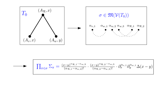
Figure 2: From trees to OPE coefficients: Given a tree $T_{0}$ [top left] with multi-index labels $A_{v}=(\alpha_{v,1}),A_{w}=(\alpha_{w,1},\alpha_{w,2},\alpha_{w,3})$ and $A_{\mathcal{R}}=(\alpha_{\mathcal{R},1},\alpha_{\mathcal{R},2})$, we obtain perfect matchings $\sigma\in\mathfrak{M}(\mathcal{V}(T_{0}))$ [top right] by decomposing the indices $(\alpha_{v,1},\alpha_{w,1},\alpha_{w,2},\alpha_{w,3},\alpha_{\mathcal{R},1},\alpha_{\mathcal{R},2})$ into pairs. The contribution to the OPE coefficient $({\mathcal{P}}_{0})(T_{0})=(\mathcal{C}_{0})_{A_{w}A_{v}}^{A_{\mathcal{R}}}(y,x)$ corresponding to a perfect matching $\sigma$ is given according to eq.(4.61) by explicit expressions involving the propagator $\Delta$ [bottom].

We now want to extend this representation to more complicated trees $T$. As a warm up, let us first consider trees $T_{1}$ with only one internal vertex $u$ besides the root, $\mathcal{I}_{\mathcal{R}}=\{u\}$, such as the tree displayed in fig.1. As mentioned earlier in (3.51), trees of this type correspond to a product of two OPE coefficients, $(\mathcal{C}_{0})_{(A_{v})_{v\in\operatorname{ch}(u)}}^{A_{u}}(\mathcal{C}_{0})_{(A_{v})_{v\in\operatorname{ch}(\mathcal{R})}}^{A_{\mathcal{R}}}$. Using the representation (4.60), we can express this product in terms of two weighted perfect matchings:

$$\sum_{[A_{u}]=D}({\mathcal{P}}_{0})(T_{1})=\sum_{[A_{u}]=D}\Big{(}\sum_{\sigma_{1}\in\mathfrak{M}(\mathcal{V}(T_{1}^{1}))}\prod_{\pi_{1}\in\sigma_{1}}\Sigma_{\pi_{1}}\Big{)}\,\cdot\,\Big{(}\sum_{\sigma_{2}\in\mathfrak{M}(\mathcal{V}(T_{1}^{2}))}\prod_{\pi_{2}\in\sigma_{2}}\Sigma_{\pi_{2}}\Big{)}$$ (4.63)

Here we write $T_{1}^{a}$ for the tree which is obtained from $T_{1}$ by deleting all vertices and edges above the internal vertex $u\in\mathcal{I}_{\mathcal{R}}$, and $T_{1}^{b}$ for the tree which results from $T_{1}$ by deleting all vertices and edges below $u\in\mathcal{I}_{\mathcal{R}}$, see fig.3.

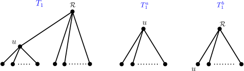
Figure 3: The decomposition of a tree $T_{1}$ into subtrees $T_{1}^{a},T_{1}^{b}$ without internal vertices.

Equation (4.63) can be simplified in various ways. Firstly, we note that the internal vertex $u\in\mathcal{I}_{\mathcal{R}}$ appears in both matchings, which we can highlight by writing the above equation as follows:

$$\sum_{[A_{u}]=D}({\mathcal{P}}_{0})(T_{1})=\sum_{\begin{subarray}{c}\sigma_{1}\in\mathfrak{M}(\mathcal{V}(T_{1}^{a}))\\ \sigma_{2}\in\mathfrak{M}(\mathcal{V}(T_{1}^{b}))\end{subarray}}\prod_{\begin{subarray}{c}[(v,i),(w,j)]\in\sigma_{1}\cup\sigma_{2}\\ v,w\neq u\end{subarray}}\Sigma_{(v,i),(w,j)}\sum_{[A_{u}]=D}\prod_{\begin{subarray}{c}[(v,i),(u,k)]\in\sigma_{1}\\ [(u,k),(w,j)]\in\sigma_{2}\end{subarray}}\Sigma_{(v,i),(u,k)}\cdot\Sigma_{(u,k),(w,j)}$$ (4.64)

The product on the very right, which contains all matchings involving the internal $u$-vertex, can then be written as

$$\begin{split}&\sum_{|\alpha_{u,k}|=d}\Sigma_{(v,i)(u,k)}\cdot\Sigma_{(u,k)(w,j)}\\ &=\begin{cases}\sum\limits_{|\alpha_{u,k}|=d}\frac{\partial^{\alpha_{v,i}}_{x_{v}}(x_{v}-x_{u})^{\alpha_{u,k}}}{\alpha_{u,k}!}\,\partial^{\alpha_{u,k}}_{x_{u}}\partial^{\alpha_{w,j}}_{x_{w}}\Delta(x_{u}-x_{w})={\mathbb{T}}_{x_{v}\to x_{u}}^{d-|\alpha_{v,i}|}\Sigma_{(v,i)(w,j)}&w\neq\mathcal{R}\\ \sum\limits_{|\alpha_{u,k}|=d}\frac{\partial^{\alpha_{v,i}}_{x_{v}}(x_{v}-x_{u})^{\alpha_{u,k}}}{\alpha_{u,k}!}\,\frac{\partial^{\alpha_{u,k}}_{x_{u}}(x_{u}-x_{\mathcal{R}})^{\alpha_{w,j}}}{\alpha_{w,j}!}={\mathbb{T}}_{x_{v}\to x_{u}}^{d-|\alpha_{v,i}|}\Sigma_{(v,i)(w,j)}&w=\mathcal{R}\end{cases}\end{split}$$ (4.65)

where ${\mathbb{T}}^{d}$ is the Taylor expansion operator

$${\mathbb{T}}_{x\to y}^{d}f(x):=\begin{cases}\sum_{|v|=d}\frac{(x-y)^{v}}{v!}\,\partial^{v}_{y}f(y)&\text{ for }d\geq 0\\ 0&\text{ for }d<0\,.\end{cases}$$ (4.66)

We can further simplify eq.(4.64) by expressing the summation over the matchings $\sigma_{1},\sigma_{2}$ in terms of matchings $\sigma\in\mathfrak{M}(\mathcal{L}\cup\mathcal{R}(T_{1}))$. This is achieved by merging the two matchings at the $(u,k)$ vertices, as shown in fig.4.

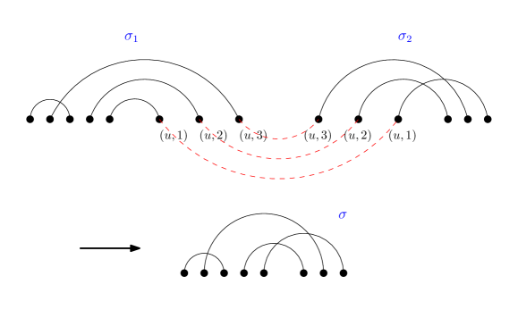
Figure 4: Given two perfect matchings $\sigma_{1}\in\mathfrak{M}(\mathcal{V}(T_{1}^{a})),\sigma_{2}\in\mathfrak{M}(\mathcal{V}(T_{1}^{b}))$ [top] we obtain a matching $\sigma\in\mathfrak{M}(\mathcal{L}\cup\mathcal{R}(T_{1}))$ [bottom] by merging the vertices corresponding to the internal vertex $u\in\mathcal{I}_{\mathcal{R}}(T_{1})$ as indicated by the dashed red lines.

Note however that this mapping $(\sigma_{1},\sigma_{2})\to\sigma$ is not one to one: Exchanging two vertices $(u,k)$ and $(u,k^{\prime})$ yields the same matching $\sigma$. For a given $\sigma$, we therefore pick up a symmetry factor $|I(\sigma)|!$, where (recall that $\operatorname{de}(u)$ denotes the descendants of $u$)

$$I(\sigma):=\{[(v,i)(w,j)]\in\sigma\,:\,v\in\operatorname{de}(u),w\notin\operatorname{de}(u)\}$$ (4.67)

is the set of merged edges, i.e. those adjacent to a $u$-vertex in the original matchings $\sigma_{1},\sigma_{2}$. The matching procedure thus leads to the formula

$$\sum_{[A_{u}]=D}({\mathcal{P}}_{0})(T_{1})=\sum_{\sigma\in\mathfrak{M}(\mathcal{L}\cup\mathcal{R}(T_{1}))}|I(\sigma)|!\sum_{\vec{d}\in\mathcal{D}(\sigma)}\prod_{\pi=[(v,i)(w,j)]\in\sigma}\begin{cases}{\mathbb{T}}_{x_{v}\to x_{u}}^{d_{\pi}-|\alpha_{v,i}|}\Sigma_{\pi}&\text{ if }\pi\in I(\sigma),v\in\operatorname{ch}(u)\\ \Sigma_{\pi}&\text{ if }\pi\notin I(\sigma)\end{cases}$$ (4.68)

where we summarised the possible assignments of the Taylor expansion degrees to the merged lines in the definition

$$\mathcal{D}(\sigma)=\{\vec{d}=(d_{\pi})_{\pi\in I(\sigma)}\,:\,d_{\pi}\in\mathbb{N},\sum_{\pi\in I(\sigma)}(d_{\pi}+1)=D\}\,.$$ (4.69)

We can generalise this strategy to the expression $({\mathcal{P}}_{0})(T)$ for more complicated trees $T$. For this purpose, let us first define the sets

$${I}_{u}(\sigma):=\{[(v,i)(w,j)]\in\sigma\,:\,v\in\operatorname{de}(u),w\notin\operatorname{de}(u)\}$$ (4.70)

for any $u\in\mathcal{I}_{\mathcal{R}}$, which contain all edges which are merged by connecting two $u$-vertices. Further, define

$$\mathcal{D}(\sigma)=\{\vec{d}=(d^{u}_{\pi})^{u\in\mathcal{I}_{\mathcal{R}}}_{\pi\in I_{u}(\sigma)}\,:\,d^{u}_{\pi}\in\mathbb{N},\sum_{\pi\in I_{u}(\sigma)}(d^{u}_{\pi}+1)=D_{u}\}\,,$$ (4.71)

which is the set of all assignments of the Taylor expansion degrees to the merged edges. We then have the compact formula:

Lemma 2.

Let $T\in\mathcal{T}(\vec{x};\vec{A})$. Then

$$\prod_{u\in\mathcal{I}_{\mathcal{R}}(T)}\sum_{[A_{u}]=D_{u}}({\mathcal{P}}_{0})(T)=\sum_{\sigma\in\mathfrak{M}(\mathcal{L}\cup\mathcal{R}(T))}\prod_{u\in\mathcal{I}_{\mathcal{R}}(T)}|I_{u}(\sigma)|!\sum_{\vec{d}\in\mathcal{D}(\sigma)}\prod_{\pi\in\sigma}M_{\pi}(\vec{d})$$ (4.72)

where the matrix $M(\vec{d})$ is given by (recall that by $\operatorname{an}(v)$ we denote ancestors of $v$)

$$M_{\pi=[(v,i)(w,j)]}(\vec{d})=\prod_{u\in\operatorname{an}(v)\setminus\operatorname{an}(w)}{\mathbb{T}}_{x_{v}\to x_{u}}^{d_{\pi}^{u}-|\alpha_{v,i}|}\,\prod_{s\in\operatorname{an}(w)\setminus\operatorname{an}(v)}{\mathbb{T}}_{x_{w}\to x_{s}}^{d_{\pi}^{s}-|\alpha_{w,j}|}\quad\Sigma_{\pi}$$ (4.73)

The product over the vertices $u,s$ in eq.(4.73) is ordered from leaf to root, i.e. every vertex is to the left of its ancestors.

Proof.

The proof works by induction in the number of internal vertices $|\mathcal{I}_{\mathcal{R}}(T)|$. In the simple examples above we have already dealt with the cases $|\mathcal{I}_{\mathcal{R}}(T_{0})|=0$ and $|\mathcal{I}_{\mathcal{R}}(T_{1})|=1$, so the induction start has already been taken care of. The induction step works as follows: Assuming that lemma 2 holds for all trees $T^{\prime}\in\mathcal{T}(\vec{x};\vec{A})$ with up to $n$ internal vertices, $|\mathcal{I}_{\mathcal{R}}(T^{\prime})|\leq n$, we have to show that the lemma also holds for trees $T$ with $n+1$ internal vertices, i.e. for $|\mathcal{I}_{\mathcal{R}}(T)|=n+1$.

The idea of the proof is analogous to the simple example with one internal vertex discussed above: Fix any internal vertex $u\in\mathcal{I}_{\mathcal{R}}(T)$ and denote by $T^{a}$ the tree obtained from $T$ by deleting all vertices and edges above the vertex $u$, and by $T^{b}$ the tree obtained from $T$ by deleting all vertices and edges below $u$. Since both $T^{a}$ and $T^{b}$ have at most $n$ internal vertices, we can use the induction hypothesis in order to express $({\mathcal{P}}_{0})(T)$ as a product of the form

$$\begin{split}\prod_{s\in\mathcal{I}_{\mathcal{R}}(T)}\sum_{[A_{s}]=D_{s}}({\mathcal{P}}_{0})(T)=\sum_{[A_{u}]=D_{u}}&\sum_{\sigma_{a}\in\mathfrak{M}(\mathcal{L}\cup\mathcal{R}(T^{a}))}\prod_{s\in\mathcal{I}_{\mathcal{R}}(T^{a})}|I_{s}(\sigma_{a})|!\sum_{\vec{d}_{a}\in\mathcal{D}(\sigma_{a})}\prod_{\pi_{a}\in\sigma_{a}}M_{\pi_{a}}(\vec{d}_{a})\\ \times&\sum_{\sigma_{b}\in\mathfrak{M}(\mathcal{L}\cup\mathcal{R}(T^{b}))}\prod_{s\in\mathcal{I}_{\mathcal{R}}(T^{b})}|I_{s}(\sigma_{b})|!\sum_{\vec{d}_{b}\in\mathcal{D}(\sigma_{b})}\prod_{\pi_{b}\in\sigma_{b}}M_{\pi_{b}}(\vec{d}_{b})\end{split}$$ (4.74)

From here on we can essentially repeat the discussion following eq.(4.63): We distinguish matchings in $\sigma_{a}$ and $\sigma_{b}$ containing the vertex $u$, and those that do not. For the former, we obtain products of the form $M_{(v,i),(u,k)}(\vec{d}_{a})M_{(u,k),(w,j)}(\vec{d}_{b})$, which can be simplified using eq.(4.65):

$$\sum_{|\alpha_{u,k}|=d_{\pi}^{u}}M_{(v,i),(u,k)}(\vec{d}_{a})\cdot M_{(u,k),(w,j)}(\vec{d}_{b})=M_{(v,i)(w,j)}(\vec{d})$$ (4.75)

Expressing the matchings $\sigma_{a},\sigma_{b}$ in terms of matchings $\sigma\in\mathfrak{M}(\mathcal{L}\cup\mathcal{R}(T))$ by merging the $u$-vertices as before (see fig.4 and the corresponding discussion), we pick up a factor $|I_{u}(\sigma)|!$ and thereby arrive at the representation (4.72) as claimed. ∎

4.1.1 Proof of the bound (3.53) for $r=0$:

Lemma 2 provides a compact expression for the objects of interest in our proof of theorem 2. Next we would like to derive an upper bound for the r.h.s. of eq.(4.72). This is achieved with the help of the following lemma:

Lemma 3.

Let $M(\vec{d})$ be the matrix defined in eq.(4.73), let $b\in\mathcal{B}(T)$ be the branch of $T$ fixed in theorem 2, let $\pi=[(v,i)(w,j)]\in\sigma$ and define the shorthand

$$\chi_{u}:=\xi_{u}\times\begin{cases}(1+\varepsilon)&\text{ for }u\in b(T)\\ 1/\varepsilon^{2}&\text{ for }u\notin b(T)\,.\end{cases}$$ (4.76)

where $\varepsilon\in(0,2^{-\mathfrak{D}_{T}-3})$ with $\mathfrak{D}_{T}$ as defined in theorem 2. For any $\delta\geq 0$ one has the bounds

$$|M_{\pi}(\vec{d})|\leq\begin{cases}\frac{(|\alpha_{v,i}|+|\alpha_{w,j}|+\delta)!\,\prod\limits_{u\in P_{\pi}}\theta(d_{\pi}^{u}-d_{\pi}^{\operatorname{ch}(u)\cap P_{\pi}})\chi_{u}^{d_{\pi}^{u}+1}}{(\varepsilon^{2}\min\limits_{u\in\operatorname{sb}(v)}|x_{u}-x_{v}|)^{1+|\alpha_{v,i}|}(\varepsilon^{2}\min\limits_{u\in\operatorname{sb}(w)}|x_{u}-x_{w}|)^{1+|\alpha_{w,j}|}\ m^{\delta}(\varepsilon^{2}|x_{e}-x_{f}|)^{\delta}}&\text{for }v,w\neq\mathcal{R}\\ \frac{\max_{u\in\operatorname{ch}(\mathcal{R})}|x_{u}-x_{\mathcal{R}}|^{|\alpha_{w,j}|+1}}{\min_{u\in\operatorname{sb}(v)}|x_{u}-x_{v}|^{|\alpha_{v,i}|+1}}\prod_{u\in P_{\pi}}\theta(d_{\pi}^{u}-d_{\pi}^{\operatorname{ch}(u)\cap P_{\pi}})\cdot\xi_{u}^{d_{\pi}^{u}}&\text{for }w=\mathcal{R}\end{cases}$$ (4.77)

where we use the shorthand $P_{\pi}:=(\operatorname{an}(v)\setminus\operatorname{an}(w))\cup(\operatorname{an}(w)\setminus\operatorname{an}(v))$ and where $e$ is the vertex closest to the root in the set $\operatorname{an}(v)\setminus\operatorname{an}(w)$ (ancestors of $v$ which are not an ancestor of $w$), and similarly for $f$ with the roles of $v$ and $w$ exchanged.

The straightforward but tedious proof of this lemma can be found in appendix A.2. Using lemma 2 we can bound the l.h.s. of (3.53) for $r=0$.

$$\Big{|}\prod_{u\in\mathcal{I}_{\mathcal{R}}(T)}\sum_{[A_{u}]=D_{u}}({\mathcal{P}}_{0})(T)\Big{|}\leq\sum_{\sigma\in\mathfrak{M}(\mathcal{L}\cup\mathcal{R})}\prod_{u\in\mathcal{I}_{\mathcal{R}}}|I_{u}(\sigma)|!\sum_{\vec{d}\in\mathcal{D}(\sigma)}\prod_{\pi\in\sigma}\,|M_{\pi}(\vec{d})|$$ (4.78)

We would like to bound the product of matrix entries on the r.h.s. of this inequality with the help of lemma 3. For this purpose, we first note that the product of combinatoric factors can be simplified using $\sum_{\pi\in I_{u}(\sigma)}(d_{\pi}^{u}+1)=D_{u}$ and using

$$\prod_{\pi\in\sigma}(|\alpha_{v,i}|+|\alpha_{w,j}|+\delta)!\leq(\sum_{v\in\mathcal{L}}[A_{v}])!\,.$$ (4.79)

A rather non-trivial point concerns the factors $m^{\delta}|x_{e}-x_{f}|^{\delta}$ in the bound (4.77). How many of these factors do we obtain in the product over $\pi\in\sigma$? Note that, on account of the $\theta$-functions, our bound (4.77) on the matrix elements $M_{\pi}$ vanishes if $\vec{d}\in\mathcal{D}(\sigma)$ contains two elements $d_{\pi}^{e}<d_{\pi}^{f}$ such that $e$ is closer to the root of $T$ than $f$. Pick a vertex $u\in\mathcal{I}(T)$. If we have $\Delta(u)>0$ at that vertex, then there has to be at least one pair $[(v,i)(w,j)]=\pi\in\sigma$ such that $v,w\in\operatorname{de}(u)$ for the product of matrix elements not to vanish, since otherwise we would have a pair $d_{\pi}^{u}<d_{\pi}^{\operatorname{ch}(u)}$. From lemma 3 we know that in this case, since clearly $v,w\neq\mathcal{R}$, we have the freedom to generate an additional power of $1/(m\cdot\min_{e,e^{\prime}\in\operatorname{ch}(u)}|x_{e}-x_{e^{\prime}}|)^{\delta_{u}}$. Repeating this argument at every internal vertex of $T$, we arrive at the bound

$$\prod_{\pi\in\sigma}\,|M_{\pi}(\vec{d})|\leq\frac{\max\limits_{u\in\operatorname{ch}(\mathcal{R})}|x_{u}-x_{\mathcal{R}}|^{[A_{\mathcal{R}}]}\,(\sum\limits_{v\in\mathcal{L}}[A_{v}])!\,\varepsilon^{-2\sum_{v\in\mathcal{V}\setminus b(T)}[A_{v}]}(1+\varepsilon)^{\sum_{w\in b(T)}[A_{w}]}}{\prod\limits_{v\in\mathcal{L}}\min\limits_{u\in\operatorname{sb}(v)}|x_{u}-x_{v}|^{[A_{v}]}\prod\limits_{u\in\mathcal{I}}(m\cdot\min\limits_{i,j\in\operatorname{ch}(u)}|x_{i}-x_{j}|)^{\theta(\Delta_{u})\cdot\delta_{u}}}\prod_{i\in\mathcal{I}_{\mathcal{R}}}\xi^{D_{i}}_{i}\,.$$ (4.80)

Substituting the bound (4.80) into (4.78) and using also the estimate

$$\prod_{u\in\mathcal{I}_{\mathcal{R}}}|I_{u}(\sigma)|!\leq\textbf{n}!^{{|\mathcal{I}_{\mathcal{R}}|}}$$ (4.81)

where $\textbf{n}:=\sum_{v\in\mathcal{L}\cup\mathcal{R}}n_{v}\leq\mathfrak{D}_{T}$ with $n_{v}$ as defined in (4.59), as well as

$$|\mathfrak{M}(\mathcal{L}\cup\mathcal{R})|=(\textbf{n}-1)!!\leq\textbf{n}!$$ (4.82)

and

$$|\mathcal{D}(\sigma)|\leq\prod_{u\in\mathcal{I}_{\mathcal{R}}}(D_{u}+1)^{\textbf{n}}\leq 2^{\textbf{n}\sum_{v\in\mathcal{I}_{\mathcal{R}}\setminus b}D_{v}}\prod_{u\in b(T)}(D_{u}+1)^{\textbf{n}}\leq\varepsilon^{-\sum_{v\in\mathcal{V}\setminus b}[A_{v}]}\prod_{u\in b(T)}(D_{u}+1)^{\mathfrak{D}_{T}}\,,$$ (4.83)

to bound the summations over $\sigma\in\mathfrak{M}(\mathcal{L}\cup\mathcal{R})$ and over $\vec{d}\in\mathcal{D}(\sigma)$ in (4.78), we finally arrive at a bound for the quantities of interest:

$$\begin{split}\Big{|}\prod_{u\in\mathcal{I}_{\mathcal{R}}(T)}\sum_{[A_{u}]=D_{u}}({\mathcal{P}}_{0})(T)\Big{|}&\leq\frac{\max\limits_{u\in\operatorname{ch}(\mathcal{R})}|x_{u}-x_{\mathcal{R}}|^{[A_{\mathcal{R}}]}}{\prod\limits_{v\in\mathcal{L}}\min\limits_{u\in\operatorname{sb}(v)}|x_{u}-x_{v}|^{[A_{v}]}\prod\limits_{u\in\mathcal{I}}(m\cdot\min\limits_{i,j\in\operatorname{ch}(u)}|x_{i}-x_{j}|)^{\theta(\Delta_{u})\cdot\delta_{u}}}\prod_{u\in\mathcal{I}_{\mathcal{R}}}\xi^{D_{u}}_{u}\\ &\times\textbf{n}!^{|\mathcal{I}_{\mathcal{R}}|+1}\cdot(\sum_{v\in\mathcal{L}}[A_{v}])!\,\varepsilon^{-3\sum_{v\in\mathcal{V}\setminus b(T)}[A_{v}]}\,\prod_{w\in b}(D_{w}+1)^{\mathfrak{D}_{T}}(1+\varepsilon)^{[A_{w}]}\end{split}$$ (4.84)

This inequality indeed implies the bound (3.53) for the free field ($r=0$) if we choose the constant $K$ such that $K\geq\textbf{n}!^{|\mathcal{I}_{\mathcal{R}}|+1}\cdot(\sum_{v\in\mathcal{L}}[A_{v}])!$.

4.1.2 Proof of the convergence relation (3.55) for $r=0$:

To complete the induction start, it remains to be shown that the convergence property (3.55) holds for the free theory, i.e. we need to show that (suppressing for the moment the dependence on the coordinates $x_{i}$)

$$\lim_{D\to\infty}(R_{0}^{D})_{A_{1}\ldots A_{M};A_{M+1}\ldots A_{N}}^{B}=(\mathcal{C}_{0})_{A_{1}\ldots A_{N}}^{B}-\sum_{[C]=0}^{\infty}(\mathcal{C}_{0})_{A_{1}\ldots A_{M}}^{C}(\mathcal{C}_{0})_{CA_{M+1}\ldots A_{N}}^{B}=0$$ (4.85)

on the domain $\xi<1$ defined by (1.11). In terms of our tree notation, we can write the associativity remainder as

$$(R_{0}^{D})_{A_{1}\ldots A_{M};A_{M+1}\ldots A_{N}}^{B}=({\mathcal{P}}_{0})(T_{0})-\sum_{d\leq D}\sum_{[C]=d}({\mathcal{P}}_{0})(T_{1})\,,$$ (4.86)

where $T_{0}\in\mathcal{T}((A_{1},\ldots,A_{N},B);(x_{1},\ldots,x_{N}))$ and $T_{1}\in\mathcal{T}((A_{1},\ldots,A_{N},B,C);(x_{1},\ldots,x_{N}))$ are the trees shown in figure 1. Using the bound (4.84) for the r.h.s. of this equation, one can verify that the sum over $d$ is absolutely convergent on the domain $\xi<1$ in the limit $D\to\infty$ [see the discussion following eq.(3.56)].

Thus, it remains to show that the limit in eq.(4.85) is indeed zero. To see this, we recall equation (4.68), which we can write in the limit $D\to\infty$ and for $\xi<1$ as (using the Leibniz rule to pull Taylor expansions out of the product)

$$\sum_{[C]=0}^{\infty}(\mathcal{C}_{0})_{A_{1}\ldots A_{M}}^{C}\,(\mathcal{C}_{0})_{CA_{M+1}\ldots A_{N}}^{B}=\sum_{\sigma\in\mathfrak{M}(\mathcal{L}\cup\mathcal{R}(T_{1}))}\prod_{\pi\in\sigma\setminus I(\sigma)}\Sigma_{\pi}\sum_{d=0}^{\infty}{\mathbb{T}}_{(x_{1},\ldots,x_{M})\to(x_{M},\ldots,x_{M})}^{d}\prod_{\pi^{\prime}\in I(\sigma)}\Sigma_{\pi^{\prime}}$$ (4.87)

Here ${\mathbb{T}}_{(x_{1},\ldots,x_{M})\to(x_{M},\ldots,x_{M})}^{d}$ is the multivariate Taylor operator,

$${\mathbb{T}}_{(x_{1},\ldots,x_{M})\to(x_{M},\ldots,x_{M})}^{d}f(x_{1},\ldots,x_{M})=\sum_{|v_{1}|+\ldots+|v_{M}|=d}\prod_{i=1}^{M}\frac{(x_{i}-x_{M})^{v_{i}}}{v_{i}!}\,\partial_{y_{i}}^{v_{i}}f(y_{1},\ldots,y_{M})\Big{|}_{y_{i}\to x_{M}}\,.$$ (4.88)

Using the fact that the Taylor series is convergent on the mentioned domain and recalling our explicit formula (4.60) for the zeroth order OPE coefficients, we therefore arrive at the relation

$$\sum_{[C]=0}^{\infty}(\mathcal{C}_{0})_{A_{1}\ldots A_{M}}^{C}\,(\mathcal{C}_{0})_{CA_{M+1}\ldots A_{N}}^{B}=\sum_{\sigma\in\mathfrak{M}(\mathcal{V}(T_{0}))}\prod_{\pi\in\sigma}\Sigma_{\pi}=(\mathcal{C}_{0})_{A_{1}\ldots A_{N}}^{B}\,,$$ (4.89)

which establishes equation (3.55) for the free field and thereby concludes the induction start.

4.2 Induction step: Higher perturbation orders

Assuming that theorem 2 holds up to perturbation order $r$, we now want to show that it also holds at order $r+1$. Our main tool to achieve this task is the recursion formula for the OPE coefficients, eq.(1.12), which in turn implies a corresponding recursion formula for the expressions $({\mathcal{P}}_{r})(T)$.

4.2.1 Proof of the bound (3.53) at order $r+1$:

When expanded in $g$, our recursion formula (1.12) reads at order $g^{r+1}$:

$$\begin{split}(\mathcal{C}_{r+1})_{A_{1}\ldots A_{N}}^{B}(x_{1},\ldots,x_{N})&=\frac{-1}{(r+1)}\int{\rm d}^{4}y\,\Big{[}(\mathcal{C}_{r})_{{\mathfrak{L}}A_{1}\ldots A_{N}}^{B}(y,x_{1},\ldots,x_{N})\\ &-\sum_{i=1}^{N}\sum_{[C]\leq[A_{i}]}\sum_{r_{1}+r_{2}=r}(\mathcal{C}_{r_{1}})_{{\mathfrak{L}}A_{i}}^{C}(y,x_{i})\,(\mathcal{C}_{r_{2}})_{A_{1}\ldots\widehat{A_{i}}C\ldots A_{N}}^{B}(x_{1},\ldots,x_{N})\\ &-\sum_{[C]<[B]}\sum_{r_{1}+r_{2}=r}(\mathcal{C}_{r_{1}})_{A_{1}\ldots A_{N}}^{C}(x_{1},\ldots,x_{N})\,(\mathcal{C}_{r_{2}})_{{\mathfrak{L}}C}^{B}(y,x_{N})\Big{]}\,,\end{split}$$ (4.90)

where the index ${\mathfrak{L}}$ corresponds to the interaction operator of our model, i.e. ${\mathcal{O}}_{{\mathfrak{L}}}:=\varphi^{4}/4!$. Formula (4.90) allows us to write the l.h.s. of (3.53) at order $r+1$ in terms of $r$-th order quantities via

$$\begin{split}&\prod_{i\in\mathcal{I}_{\mathcal{R}}}\sum_{[A_{i}]=D_{i}}({\mathcal{P}}_{r+1})(T)=\frac{-1}{r+1}\prod_{i\in\mathcal{I}_{\mathcal{R}}}\sum_{[A_{i}]=D_{i}}\sum_{\sum_{u\in\mathcal{I}}r_{u}=r+1}\prod_{v\in\mathcal{I}}(\mathcal{C}_{r_{v}})_{(A_{w})_{w\in\operatorname{ch}(v)}}^{A_{v}}((x_{i})_{i\in\operatorname{ch}(v)};x_{v})\\ &=\frac{-1}{r+1}\prod_{i\in\mathcal{I}_{\mathcal{R}}}\sum_{[A_{i}]=D_{i}}\sum_{v\in\mathcal{I}}\int_{y}\Big{[}({\mathcal{P}}_{r})(T_{v})-\sum_{w\in\operatorname{ch}(v)}\sum_{[A_{u}]\leq[A_{w}]}({\mathcal{P}}_{r})(T_{w,A_{u}})-\sum_{[A_{u}]<[A_{v}]}({\mathcal{P}}_{r})(T_{A_{u},v})\Big{]}\end{split}$$ (4.91)

where the trees $T_{v},T_{v,A_{u}},T_{A_{u},v}$ are obtained form $T\in\mathcal{T}(\vec{x};\vec{A})$ as follows (see fig.5):

• $T_{v}\in\mathcal{T}((\vec{x},y);(\vec{A},{\mathfrak{L}}))$ is obtained from $T$ by connecting an additional leaf with weight $({\mathfrak{L}},y)$ to the vertex $v$.

• $T_{v,A_{u}}\in\mathcal{T}((\vec{x},y);(\vec{A},{\mathfrak{L}},A_{u}))$ is obtained by connecting a leaf with weight $({\mathfrak{L}},y)$ to the parent edge of $v$, splitting this edge into two halves. The new vertex $u$ adjacent to these two halves receives the weight $(A_{u},x_{v})$.

• $T_{A_{u},v}\in\mathcal{T}((\vec{x},y);(\vec{A},{\mathfrak{L}},A_{u}))$ is obtained by connecting a leaf with weight $({\mathfrak{L}},y)$ to the parent edge of $v$, splitting this edge into two halves (if $v=\mathcal{R}$, then we add a parent edge to $v$ and connect the leaf to this new root). The new vertex $u$ adjacent to these two halves receives the weight $(A_{v},x_{v})$, and we change the weight of the vertex $v$ to $(A_{u},x_{v})$.

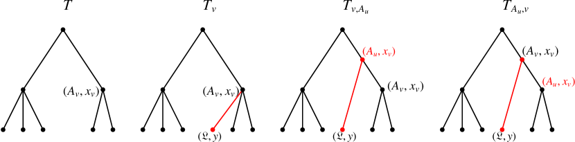
Figure 5: The trees $T_{v},T_{v,A_{u}},T_{A_{u},v}$ are obtained from the tree $T$ by adding an external edge.

Our plan is now to combine the formula (4.91) with the inductive bound (3.53), which holds up to order $r$ by assumption, in order to verify the bound (3.53) at order $r+1$. The terms under the integral in eq.(4.91) can be estimated with the help of the following bounds:

Lemma 4.

Denote by $B_{r}(T)$ the r.h.s. of (3.53). Then

$$\Big{|}\prod_{i\in\mathcal{I}_{\mathcal{R}}}\sum_{[A_{i}]=D_{i}}({\mathcal{P}}_{r})(T_{v})\Big{|}\leq\frac{B_{r}(T)\,K}{\min\limits_{w\in\operatorname{ch}(v)}|x_{w}-y|^{4}}\sup\left(\frac{\min\limits_{i,j\in\operatorname{ch}(v)}|x_{j}-x_{i}|}{\min\limits_{i\in\operatorname{ch}(v)}|y-x_{i}|},\frac{|y-x_{v}|}{\max\limits_{i\in\operatorname{ch}(v)}|x_{i}-x_{v}|},1\right)^{2\delta_{v}}$$

$$\times\left(\frac{\prod_{w\in b}(D_{w}+1)}{\varepsilon}\right)^{4\cdot 8^{r+1}}\prod_{i\in\operatorname{ch}(v)}\sup\left(\frac{\min\limits_{j\in\operatorname{ch}(v)\setminus\{i\}}|x_{j}-x_{i}|}{|y-x_{i}|},1\right)^{[A_{i}]}\sup\left(\frac{|y-x_{v}|}{\max\limits_{j\in\operatorname{ch}(v)\setminus\{i\}}|x_{j}-x_{v}|},1\right)^{[A_{v}]}$$ (4.92)

$$\Big{|}\sum_{[A_{u}]=d}\prod_{i\in\mathcal{I}_{\mathcal{R}}}\sum_{[A_{i}]=D_{i}}({\mathcal{P}}_{r})(T_{v,A_{u}})\Big{|} \leq\frac{B_{r}(T)\,K\sup(1,1/m|x_{v}-y|)^{\delta_{u}}}{m^{\theta([A_{v}]+4-d)\delta_{u}}|x_{v}-y|^{4+\theta([A_{v}]+4-d)\delta_{u}}}\left(\frac{\min\limits_{i\in\operatorname{sb}(v)}|x_{v}-x_{i}|}{|y-x_{v}|}\right)^{[A_{v}]-d}$$

$$\times\sup\left(\frac{\min\limits_{i\in\operatorname{sb}(v)}|x_{i}-x_{v}|}{|y-x_{v}|},1\right)^{\delta_{\operatorname{pa}(v)}}\left(\frac{\prod_{w\in b}(D_{w}+1)}{\varepsilon}\right)^{4\cdot 8^{r+1}}\chi(v,d)$$ (4.93)

$$\Big{|}\sum_{[A_{u}]=d}\prod_{i\in\mathcal{I}_{\mathcal{R}}}\sum_{[A_{i}]=D_{i}}({\mathcal{P}}_{r})(T_{A_{u},v})\Big{|} \leq\frac{B_{r}(T)\,K\sup(1,1/m|x_{v}-y|)^{\delta_{u}}}{m^{\theta(d+4-[A_{v}])\delta_{u}}|x_{v}-y|^{4+\theta(d+4-[A_{v}])\delta_{u}}}\left(\frac{|y-x_{v}|}{\max\limits_{i\in\operatorname{ch}(v)}|x_{v}-x_{i}|}\right)^{[A_{v}]-d}$$

$$\times\sup\left(\frac{\min\limits_{i\neq j\in\operatorname{ch}(v)}|x_{i}-x_{j}|}{|y-x_{v}|},1\right)^{\delta_{v}}\left(\frac{\prod_{w\in b}(D_{w}+1)}{\varepsilon}\right)^{4\cdot 8^{r+1}}\chi(v,d)$$ (4.94)

where $K>0$ is a constant that depends neither on the integers $D_{i}$ nor on $\varepsilon$ or the $\delta_{v}$, and where we use the shorthand

$$\chi(v,d)=\begin{cases}(1+\varepsilon)^{8^{r+1}\,d}\cdot(d+1)^{8^{r+1}(\mathfrak{D}_{T}+4)}&\text{if }v\in b\\ \varepsilon^{-8^{r+1}d}&\text{if }v\notin b\,.\end{cases}$$ (4.95)

Proof.

The lemma follows by straightforward computation from the inductive bound (3.53). ∎

We now substitute these bounds under the integral in the recursion formula (4.91). It is, however, not possible to estimate the resulting individual terms directly, because the integral over each individual term contains divergences in the regions where $y\approx x_{i}$ (UV) or where $|y|\gg\sup_{i}|x_{i}|$ (IR). As mentioned in our overview of the proof at the beginning of this section, we therefore have to take a little more care and take into account cancellations between these divergent terms for each of those dangerous regions. In order to study these cancellations of singularities at short- and large distances, we define the following partition of $\mathbb{R}^{4}$:

Definition 5 (Integration regions).

Let $v\in\mathcal{I}(T)$ be an internal vertex of the tree $T$ and let $b\in\mathcal{B}(T)$ be the branch mentioned in theorem 2. Then

(UV-regions)

$$\Omega^{v}_{i}:=\begin{cases}\left\{y\in\mathbb{R}^{4}\,:\,|x_{i}-y|\cdot(1+\varepsilon)^{2\cdot 8^{r+1}}<\min_{j\in\operatorname{sb}(i)}|x_{i}-x_{j}|\right\}&\text{ if }i\in\operatorname{ch}(v)\cap b(T)\\ &\\ \left\{y\in\mathbb{R}^{4}\,:\,|x_{i}-y|\cdot\varepsilon^{-2\cdot 8^{r+1}}<\min_{j\in\operatorname{sb}(i)}|x_{i}-x_{j}|\right\}&\text{ if }i\in\operatorname{ch}(v)\setminus b(T)\\ \end{cases}$$ (4.96)

(IR-region)

$$\Omega^{v}_{IR}:=\begin{cases}\{y\in\mathbb{R}^{4}\,:\,|x_{v}-y|\geq\max\limits_{j\in\operatorname{ch}(v)}|x_{v}-x_{j}|\cdot(1+\varepsilon)^{2\cdot 8^{r+1}}\}\setminus\cup_{i}\Omega^{v}_{i}&\text{if }\operatorname{pa}(v)\in b(T)\\ &\\ \{y\in\mathbb{R}^{4}\,:\,|x_{v}-y|\geq\max\limits_{j\in\operatorname{ch}(v)}|x_{v}-x_{j}|\cdot\varepsilon^{-2\cdot 8^{r+1}}\}\setminus\cup_{i}\Omega^{v}_{i}&\text{if }\operatorname{pa}(v)\notin b(T)\\ \end{cases}$$ (4.97)

(Intermediate region)

$$\Omega^{v}_{IM}:=\mathbb{R}^{4}\setminus(\cup_{i}\Omega^{v}_{i}\cup\Omega^{v}_{IR})$$ (4.98)

Remark:

Note that for any $v\in\mathcal{I}(T)$ one has $\Omega_{IM}^{v}\cup\Omega_{IR}^{v}\cup_{i\in\operatorname{ch}(v)}\Omega_{i}^{v}=\mathbb{R}^{4}$ and that these sets are disjoint, in particular $\Omega^{v}_{i}\cap\Omega^{v}_{j}=\emptyset$ if $i\neq j$. Note further that the UV- and IR-regions get smaller as we increase the perturbation order, which will be needed later in order to obtain sufficiently strong bounds within those regions [more precisely, this fact is going to be crucial for the estimates (4.106) and (4.112)].

We now derive a bound on the r.h.s. of (4.91) by decomposing the $y$-integral into integrals over the regions defined above. We will see that, indeed, the resulting bounds for the contributions from each of those regions are consistent with (3.53) at order $r+1$.

The intermediate distance region $\Omega^{v}_{IM}$:

In this region the integration variable $y$ of eq.(4.91) is neither very close to, nor very far from the points $(x_{i})_{i\in\operatorname{ch}(v)}$. Hence, we will encounter neither UV- nor IR-divergences, and we can simply insert the bounds from lemma 4 in order to estimate the integrand, without taking into account any further cancellations.

Let us fix an internal vertex $v\in\mathcal{I}(T)$. By definition, we then have for any $e\in\operatorname{ch}(v)$

$$\frac{\min_{i\in\operatorname{ch}(v)}|x_{e}-x_{i}|}{|y-x_{e}|}\leq\begin{cases}(1+\varepsilon)^{2\cdot 8^{r+1}}&\text{ for }e\in b(T)\\ \varepsilon^{-2\cdot 8^{r+1}}&\text{ for }e\notin b(T)\end{cases}\Bigg{\}}\geq\frac{|y-x_{e}|}{\max_{i\in\operatorname{ch}(v)}|x_{e}-x_{i}|}\,.$$ (4.99)

Furthermore, we have the inequality

$$\begin{split}\int\limits_{\Omega^{v}_{IM}}\frac{{\rm d}^{4}y}{\min\limits_{i\in\operatorname{ch}(v)}|y-x_{i}|^{4}}&\leq\frac{(2\pi)^{2}}{\varepsilon^{2\delta\cdot 8^{r+1}}}\sum_{i\in\operatorname{ch}(v)}\int\limits_{0}^{\frac{|x_{i}-x_{v}|}{\varepsilon^{2\cdot 8^{r+1}}}}\frac{\,{\rm d}|y|}{|y|^{1-\delta}\min\limits_{j\in\operatorname{sb}(i)}|x_{i}-x_{j}|^{\delta}}\\ &\leq(2\pi)^{2}\,\textbf{n}\,\left(\frac{\max\limits_{i\in\operatorname{ch}(v)}|x_{i}-x_{v}|}{\varepsilon^{4\cdot 8^{r+1}}\!\!\min\limits_{i\neq j\in\operatorname{ch}(v)}|x_{i}-x_{j}|}\right)^{\delta}\end{split}$$ (4.100)

where as before $\textbf{n}:=\sum_{v\in\mathcal{L}\cup\mathcal{R}}n_{v}$ is the “total number of fields" associated to the external vertices of the tree $T$. Combining these inequalities with lemma 4 and choosing $\delta$ sufficiently small such that $\delta+\delta_{v}<1$, we obtain for the first term under the integral in (4.91) the bound

$$\begin{split}&\int\limits_{\Omega^{v}_{IM}}\Big{|}\prod_{i\in\mathcal{I}_{\mathcal{R}}}\sum_{[A_{i}]=D_{i}}({\mathcal{P}}_{r})(T_{v})\Big{|}\,{\rm d}^{4}y\\ &\leq B_{r}(T)\,K\,\left(\frac{\prod_{w\in b}(D_{w}+1)}{\varepsilon^{1+\delta}}\right)^{4\cdot 8^{r+1}}\left(\frac{(1+\varepsilon)^{\sum_{e\in(\operatorname{ch}(v)\cup v)\cap b}[A_{e}]}}{\varepsilon^{\sum_{e\in(\operatorname{ch}(v)\cup v)\setminus b}[A_{e}]}}\right)^{2\cdot 8^{r+1}}\left(\frac{\max\limits_{i\in\operatorname{ch}(v)}|x_{i}-x_{v}|}{\min\limits_{i\neq j\in\operatorname{ch}(v)}|x_{i}-x_{j}|}\right)^{\delta}\end{split}$$ (4.101)

where constants (i.e. factors depending neither on the weights $D_{i}$ nor on $\varepsilon$) were absorbed into $K$. The last factor on the r.h.s. can be absorbed into the expression $B_{r}(T)$ by adjusting the parameter $\delta_{v}\to\delta_{v}+\delta\in(0,1)$. To see that the resulting bound is smaller than the r.h.s. of (3.53) at order $r+1$, we note that the inductive bound (3.53) grows like

$$\begin{split}B_{r+1}(T)&=B_{r}(T)\ K\ \left(\frac{(1+\varepsilon)^{\sum_{w\in b}[A_{w}]}}{\varepsilon^{\sum_{v\in\mathcal{V}\setminus b}[A_{v}]}}\cdot\prod_{w\in b}(D_{w}+1)^{\mathfrak{D}_{T}}\right)^{7\cdot 8^{r+1}}\end{split}$$ (4.102)

as we increase the perturbation order $r$, where $K$ is some constant that depends neither on the $D_{i}$ nor on $\varepsilon$ of the $\delta_{v}$. Since the remaining terms on the r.h.s. of (LABEL:IMabound) are indeed smaller than the r.h.s. of (4.102) (choosing $\delta<1/4$ and assuming that $\sum_{v\in\mathcal{V}\setminus b}[A_{v}]>0$), we conclude that this contribution to the recursion formula (4.91) is consistent with the claimed bound (3.53).

Similarly, using lemma 4 as well as the estimates (4.99) and (4.100), we obtain for any $w\in\operatorname{ch}(v)$ the following bound on the second term under the integral in (4.91):

$$\begin{split}&\int\limits_{\Omega^{v}_{IM}}\Big{|}\sum_{[A_{u}]\leq D_{w}}\prod_{i\in\mathcal{I}_{\mathcal{R}}}\sum_{[A_{i}]=D_{i}}({\mathcal{P}}_{r})(T_{w,A_{u}})\Big{|}\,{\rm d}^{4}y\leq B_{r}(T)\,K\,\left(\frac{\prod_{i\in b}(D_{i}+1)}{\varepsilon^{2\delta_{u}+1}}\right)^{4\cdot 8^{r+1}}\\ &\quad\times\left(\frac{\max\limits_{i\in\operatorname{ch}(v)}(1/m,|x_{i}-x_{v}|)}{\min\limits_{i\neq j\in\operatorname{ch}(v)}|x_{i}-x_{j}|}\right)^{3\delta_{u}}\times\begin{cases}(D_{w}+1)^{8^{r+1}(\mathfrak{D}_{T}+4)+1}(1+\varepsilon)^{2\cdot 8^{r+1}\,(D_{w}+\delta_{v})}&\text{if }w\in b\\ (D_{w}+1)\,\varepsilon^{-2(D_{w}+\delta_{v})8^{r+1}}&\text{if }w\notin b\end{cases}\end{split}$$ (4.103)

The factor with exponent $\delta_{u}$ can again be absorbed into $B_{r}(T)$ by choosing $\delta_{u}$ sufficiently small and increasing the value of $\delta_{v}$ slightly. One checks, using also the inequality $(D_{w}+1)\leq\varepsilon^{-D_{w}}$ for the case $w\notin b$, that the bound (4.103) is indeed smaller than (4.102), and it is therefore consistent with our hypothesis (3.53). For the third term on the r.h.s. of (4.91) we can proceed in essentially the same manner as for the second one and we find that also the integral over $|\sum_{[A_{u}]\leq D_{v}}\prod_{i\in\mathcal{I}_{\mathcal{R}}}\sum_{[A_{i}]=D_{i}}({\mathcal{P}}_{r})(T_{A_{u},v})|$ satisfies the bound (4.103).

Thus, we have found that the contributions from each term under the integral are smaller than the claimed bound (3.53). In order to bound the total contribution from this integration region, it remains to estimate the number of terms appearing under the integral. For a given $v$, the integrand in (4.91) contains $|\operatorname{ch}(v)|+2\leq\textbf{n}+2$ terms. The sum over all vertices $v$ contains $|\mathcal{I}(T)|<\textbf{n}$ terms. Both of these factors can be absorbed into the constant $K$ in our bound.

To summarise, we have verified that the contribution to the r.h.s. of recursion formula (4.91) from the intermediate integration region is smaller than the claimed bound (3.53).

The UV-regions $\Omega^{v}_{i}$:

Here the integration variable $y$ is close to one of the points $x_{i}$, so we have to take into account cancellations between different terms under the integral in the recursion formula (4.91). In order to achieve this, we not only make use of the inductive bound (3.53) here, but we also apply the induction hypothesis (3.55) stated in theorem 2 in order to organise the short distance cancellations.

Fix a $v\in\mathcal{I}(T)$ and a $w\in\operatorname{ch}(v)$ and consider now $y\in\Omega_{w}^{v}$. To bound the integral over the expressions $({\mathcal{P}}_{r})(T_{A_{u},v})$ and $({\mathcal{P}}_{r})(T_{i,A_{u}})$with $i\in\operatorname{ch}(v)\setminus\{w\}$, we can proceed as above and arrive at the same bounds as in the intermediate region $y\in\Omega_{IM}^{v}$. For the two remaining terms under the integral, our second induction hypothesis, eq.(3.55), implies

$$({\mathcal{P}}_{r})(T_{v})-\sum_{[A_{u}]\leq D_{w}}({\mathcal{P}}_{r})(T_{w,A_{u}})=\sum_{[A_{u}]>D_{w}}({\mathcal{P}}_{r})(T_{w,A_{u}})\,.$$ (4.104)

To bound the r.h.s. of this equation, we now use lemma 4, distinguishing the cases $w\in b(T)$ and $w\notin b(T)$ in the process. Making use of the inequality

$$\frac{|y-x_{w}|}{\min\limits_{i\in\operatorname{sb}(w)}|x_{w}-x_{i}|}\leq\begin{cases}(1+\varepsilon)^{-2\cdot 8^{r+1}}&\text{ if }w\in b(T)\\ \varepsilon^{2\cdot 8^{r+1}}&\text{ if }w\notin b(T)\end{cases}\quad\text{ for }y\in\Omega^{v}_{w}\,,$$ (4.105)

we obtain the bound

$$\begin{split}&\int_{\Omega_{w}^{v}}\Big{|}\sum_{[A_{u}]>D_{w}}\prod_{i\in\mathcal{I}_{\mathcal{R}}}\sum_{[A_{i}]=D_{i}}({\mathcal{P}}_{r})(T_{w,A_{u}})\Big{|}\,{\rm d}^{4}y\\ &\leq\int_{\Omega^{v}_{w}}{\rm d}^{4}y\,\sum_{d=0}^{\infty}\frac{B_{r}(T)\ K\ \max(1,1/m|y-x_{w}|)^{\delta_{u}}}{|x_{w}-y|^{3+\theta(3-d)\delta_{u}}m^{\theta(3-d)\delta_{0}}\min\limits_{i\in\operatorname{sb}(w)}|x_{w}-x_{i}|}\,\left(\frac{\prod_{i\in b}([A_{i}]+1)}{\varepsilon}\right)^{4\cdot 8^{r+1}}\\ &\qquad\qquad\times\begin{cases}(1+\varepsilon)^{8^{r+1}\,(D_{w}-d+1)}(d+D_{w}+2)^{8^{r+1}(\mathfrak{D}_{T}+4)}\,&\text{ for }w\in b(T)\\ \varepsilon^{-8^{r+1}\,(D_{w}-d+1)}&\text{ for }w\notin b(T)\end{cases}\\ &\leq B_{r}(T)\,K\,\left(\frac{\prod_{i\in b}([A_{i}]+1)}{\varepsilon}\right)^{4\cdot 8^{r+1}}\,\sup\Big{(}1,\frac{1}{m\cdot\min\limits_{i\in\operatorname{sb}(w)}|x_{w}-x_{i}|}\Big{)}^{2\delta_{u}}\\ &\qquad\qquad\times\begin{cases}(1+\varepsilon)^{8^{r+1}\,(D_{w}+2)}\,\varepsilon^{-2\cdot 8^{r+1}(\mathfrak{D}_{T}+4)-2}\,(8^{r+1}(\mathfrak{D}_{T}+4))!&\text{ for }w\in b(T)\\ \varepsilon^{-8^{r+1}\,(D_{w}+1)-1}&\text{ for }w\notin b(T)\end{cases}\end{split}$$ (4.106)

Here we used the inequality

$$\sum_{d=0}^{\infty}(1+\varepsilon)^{-d\,8^{r+1}}(D_{w}+d+2)^{8^{r+1}(\mathfrak{D}_{T}+4)}\leq\frac{(1+\varepsilon)^{(D_{w}+2)8^{r+1}}}{\varepsilon^{2\cdot 8^{r+1}(\mathfrak{D}_{T}+4)+2}}\,(8^{r+1}(\mathfrak{D}_{T}+4))!$$ (4.107)

as well as the elementary estimate

$$\sum_{d=0}^{\infty}\varepsilon^{-8^{r+1}d}\leq\frac{1}{1-\varepsilon}\leq\frac{1}{\varepsilon}$$ (4.108)

to bound the infinite sums and the inequality (choosing $\delta_{u}<1/2$)

$$\int_{\Omega_{w}^{v}}\frac{\max(1,1/m|y-x_{w}|)^{\delta_{u}}\,{\rm d}^{4}y}{|x_{w}-y|^{3+\theta(3-d)\delta_{u}}m^{\theta(3-d)\delta_{u}}\min\limits_{i\in\operatorname{sb}(w)}|x_{w}-x_{i}|}\leq(2\pi)^{2}\sup\Big{(}1,\frac{1}{m\cdot\min\limits_{i\in\operatorname{sb}(w)}|x_{w}-x_{i}|}\Big{)}^{2\delta_{u}}$$ (4.109)

to bound the $y$-integral. Choosing $\delta_{u}$ small enough such that $\delta_{v}+2\delta_{u}<1$, we can absorb the factor with exponent $2\delta_{u}$ into the bound $B_{r}(T)$ via a redefinition of $\delta_{v}$. The factorial $(8^{r+1}(\mathfrak{D}_{T}+4))!$ can be absorbed into the constant $K$. As the remaining terms on the r.h.s. of (4.106) are smaller than (4.102), we conclude that also this contribution to (4.91) is consistent with our inductive bound (3.53).

To summarise, we have verified that contributions from the integral over the short distance regions $\Omega_{w}^{v}$ to the r.h.s. of (4.91) are smaller than the claimed bound (3.53).

The IR-region $\Omega^{v}_{IR}$:

Here the integration variable $y$ is far away form the points $x_{i}$, and we again have to take into account cancellations between different terms under the integral in order to bound this contribution to the recursion formula (4.91).

Fix a vertex $v\in\mathcal{I}(T)$. For the second term on the r.h.s. of (4.91) we can proceed essentially as in the case of $y\in\Omega^{v}_{IM}$ before. The only difference here is that instead of (4.100) we use the inequality

$$\int\limits_{\Omega^{v}_{IR}}\frac{{\rm d}^{4}y}{m^{\delta_{u}}|y-x_{w}|^{4+\delta_{u}}}\leq\frac{(2\pi)^{2}}{(m\min_{i\in\operatorname{sb}(w)}|x_{w}-x_{i}|)^{\delta_{u}}}$$ (4.110)

to bound the integral over $y$. This factor can be absorbed into a redefinition of $\delta_{v}$ as explained previously below (4.109).

In order to find useful bounds on the remaining terms, we again have to make use of our second induction hypothesis, eq.(3.55), which implies that

$$({\mathcal{P}}_{r})(T_{v})-\sum_{[A_{u}]<D_{v}}({\mathcal{P}}_{r})(T_{A_{u},v})=\sum_{[A_{u}]\geq D_{v}}({\mathcal{P}}_{r})(T_{A_{u},v})$$ (4.111)

for $y\in\Omega_{IR}^{v}$. Lemma 4 then implies for the r.h.s.

$$\begin{split}&\int_{\Omega^{v}_{IR}}\Big{|}\sum_{[A_{u}]\geq D_{v}}\prod_{i\in\mathcal{I}_{\mathcal{R}}}\sum_{[A_{i}]=D_{i}}({\mathcal{P}}_{r})(T_{A_{u},v})\Big{|}\,{\rm d}^{4}y\\ &\leq\int_{\Omega^{v}_{IR}}{\rm d}^{4}y\,\sum_{d=D_{v}}^{\infty}\frac{B_{r}(T)\ K\ \max(1,1/m|y-x_{v}|)^{\delta_{u}}}{|x_{v}-y|^{4+\delta_{u}}m^{\delta_{u}}}\ \left(\frac{\prod_{i\in b}([A_{i}]+1)}{\varepsilon}\right)^{4\cdot 8^{r+1}}\\ &\qquad\times\begin{cases}(1+\varepsilon)^{8^{r+1}\,(2D_{v}-d)}(d+1)^{8^{r+1}(\mathfrak{D}_{T}+4)}\,&\text{ for }v\in b(T)\\ \varepsilon^{-8^{r+1}\,(2D_{v}-d)}&\text{ for }v\notin b(T)\end{cases}\\ &\leq\frac{1}{(m\cdot\max_{j\in\operatorname{ch}(v)}|x_{v}-x_{j}|)^{\delta_{u}}}\cdot\text{r.h.s. of \eqref{uvest}}\end{split}$$ (4.112)

Here we used the same estimates as in the short-distance case to bound the sum over $d$, and we used

$$\int_{y\in\Omega^{v}_{IR}}\frac{{\rm d}^{4}y}{|x_{v}-y|^{4+\delta}}\leq\frac{(2\pi)^{2}}{\max_{j\in\operatorname{ch}(v)}|x_{v}-x_{j}|^{\delta}}\,,$$ (4.113)

to bound the $y$-integral. Choosing $\delta_{u}$ small enough, we can absorb the first factor on the r.h.s. of (4.112) into a redefinition of $\delta_{v}$. The remaining terms in the bound (4.112) are then smaller than (4.102), and we conclude that also this contribution to (4.91) is consistent with the claimed bound (3.53).

Combining our bounds for the intermediate-, UV- and IR-regions, we conclude that the r.h.s of (4.91) satisfies a bound that is smaller than our hypothesis (3.53) at order $r+1$.

4.2.2 Proof of the convergence relation (3.55) at order $r+1$:

The last step in the induction is to show, assuming that theorem 2 holds up to perturbation order $r$, that the second statement of the theorem, eq.(3.55), holds also at order $r+1$. For this purpose, we write down the recursion relation for the remainder, i.e

$$\begin{split}&\lim_{D\to\infty}(R_{r+1}^{D})_{A_{1}\ldots A_{M};A_{M+1}\ldots A_{N}}^{B}=({\mathcal{P}}_{r+1})(T_{0})-\lim_{D\to\infty}\sum_{d\leq D}\sum_{[C]=d}({\mathcal{P}}_{r+1})(T_{1})\\ &=\lim_{D\to\infty}\int_{\mathbb{R}^{4}}{\rm d}y^{4}\Bigg{\{}(\mathcal{C}_{r})_{{\mathfrak{L}}A_{1}\ldots A_{N}}^{B}-\sum_{\begin{subarray}{c}[C]\leq D\\ s\leq r\end{subarray}}(\mathcal{C}_{s})_{{\mathfrak{L}}A_{1}\ldots A_{M}}^{C}(\mathcal{C}_{r-s})_{CA_{M+1}\ldots A_{N}}^{B}\\ &-\sum_{\begin{subarray}{c}[C]\leq D\\ s\leq r\end{subarray}}(\mathcal{C}_{s})_{A_{1}\ldots A_{M}}^{C}\Bigg{(}(\mathcal{C}_{r-s})_{{\mathfrak{L}}CA_{M+1}\ldots A_{N}}^{B}-\sum_{\begin{subarray}{c}[C^{\prime}]\leq D\\ t\leq r-s\end{subarray}}(\mathcal{C}_{t})_{{\mathfrak{L}}C}^{C^{\prime}}(\mathcal{C}_{r-s-t})_{C^{\prime}A_{M+1}\ldots A_{N}}^{B}\Bigg{)}\\ &-\sum_{i=1}^{N}\sum_{\begin{subarray}{c}[C]\leq[A_{i}]\\ s\leq r\end{subarray}}(\mathcal{C}_{s})_{{\mathfrak{L}}A_{i}}^{C}\,\Bigg{(}(\mathcal{C}_{r-s})_{A_{1}\ldots\widehat{A_{i}}C\ldots A_{N}}^{B}-\sum_{\begin{subarray}{c}[C^{\prime}]\leq D\\ t\leq r-s\end{subarray}}\underbrace{(\mathcal{C}_{t})_{A_{1}\ldots A_{M}}^{C^{\prime}}(\mathcal{C}_{r-s-t})_{C^{\prime}A_{M+1}\ldots A_{N}}^{B}}_{A_{i}\to C}\Bigg{)}\\ &-\sum_{\begin{subarray}{c}[C]<[B]\\ s\leq r\end{subarray}}\Bigg{(}(\mathcal{C}_{s})_{A_{1}\ldots A_{N}}^{C}\,-\sum_{\begin{subarray}{c}[C^{\prime}]\leq D\\ t\leq s\end{subarray}}(\mathcal{C}_{t})_{A_{1}\ldots A_{M}}^{C^{\prime}}(\mathcal{C}_{s-t})_{C^{\prime}A_{M+1}\ldots A_{N}}^{C}\Bigg{)}(\mathcal{C}_{r-s})_{{\mathfrak{L}}C}^{B}\Bigg{\}}\\ \end{split}$$ (4.114)

where $T_{0}\in\mathcal{T}((A_{1},\ldots,A_{N},B);(x_{1},\ldots,x_{N}))$ and $T_{1}\in\mathcal{T}((A_{1},\ldots,A_{N},B,C);(x_{1},\ldots,x_{N}))$ are the trees depicted in fig.1. In order to show that this expression vanishes under the assumption $\xi<1$, we would like to exchange the order of the integral and the limit. By the dominated convergence theorem, this is allowed under the following conditions:

1. For all $D\in\mathbb{N}$ the integrand is bounded by some integrable function $B(y)$.

2. The limit $D\to\infty$ of the integrand converges pointwise almost everywhere.

The first condition is easily checked with the help of the bounds derived in the previous section combined with the inequality (3.57) to bound the sum over $[C]$. For the bounding function $B(y)$ we can choose for example

$$B(y):=\frac{B_{r+1}(T_{0})}{(1-\xi(1+\varepsilon)^{8^{r+1}})^{8^{r+1}\mathfrak{D}_{T}+1}}\cdot\min\left(\frac{\min|x_{i}-x_{j}|^{-1+\delta}}{\min|x_{i}-y|^{3+\delta}},\frac{m^{-\delta}}{\min|x_{i}-y|^{4+\delta}}\right)$$ (4.115)

for some $\delta\in(0,1)$ and for $\varepsilon\in(0,2^{-\mathfrak{D}_{T}-4r-3}]$, where $\mathfrak{D}_{T}=\sum_{i}[A_{i}]+[B]$. To show that the integrand converges pointwise to a limit as $D\to\infty$, we make the following observations: Using our induction hypothesis (3.55) at order $r$, it immediately follows that the last two lines of (4.114) vanish in the limit under the assumption $\xi<1$. To treat the remaining terms under the integral, we have to take a little more care: Consider first the region

$$\Omega_{1}:=\{y\in\mathbb{R}^{4}:|x_{M}-y|(1+\varepsilon)^{2\cdot 8^{r+1}}<\min_{M<j\leq N}|x_{M}-x_{j}|\,,\,|y-x_{i}|>0\}$$ (4.116)

for some small $\varepsilon>0$. In that case, the first two terms under the integral in (4.114) cancel in the limit $D\to\infty$ by our hypothesis (3.55), and the remaining terms under the integral are of the form

$$\begin{split}&\lim_{D\to\infty}\Big{|}\sum_{\begin{subarray}{c}[C]\leq D\\ s\leq r\end{subarray}}(\mathcal{C}_{s})_{A_{1}\ldots A_{M}}^{C}\Bigg{(}(\mathcal{C}_{r-s})_{{\mathfrak{L}}CA_{M+1}\ldots A_{N}}^{B}-\sum_{\begin{subarray}{c}[C^{\prime}]\leq D\\ t\leq r-s\end{subarray}}(\mathcal{C}_{t})_{{\mathfrak{L}}C}^{C^{\prime}}(\mathcal{C}_{r-s-t})_{C^{\prime}A_{M+1}\ldots A_{N}}^{B}\Bigg{)}\,\Big{|}\\ &=\lim_{D\to\infty}\big{|}\sum_{[C]\leq D}\sum_{[A_{w}]>D}({\mathcal{P}}_{r})((T_{1})_{u\in\mathcal{I}_{\mathcal{R}},A_{w}})\big{|}\leq\frac{\min|x_{i}-x_{j}|^{-1+\delta}}{\min|x_{i}-y|^{3+\delta}}\lim_{[C]\to\infty}B_{r+1}(T_{1})=0\,.\end{split}$$ (4.117)

The first equality follows simply from eq.(3.55) at order $r$, and the estimate in the third line follows analogously to our discussion of the short distance region in section 4.2.1 [see (4.106)]. Thus, we find that for $y\in\Omega_{1}$ the integrand converges to 0 as $D\to\infty$.

In the region

$$\Omega_{2}:=\{y\in\mathbb{R}^{4}:|x_{M}-y|\geq(1+\varepsilon)^{2\cdot 8^{r+1}}\max_{1\leq j\leq M}|x_{M}-x_{j}|\,,\,|y-x_{i}|>0\}$$ (4.118)

we simply exchange the role of the second and third term on the r.h.s. of (4.114) and otherwise proceed in a similar manner, using estimates from the previous discussion of the large distance region $\Omega_{IR}$ [see (4.112)]. We find that the integrand also vanishes in this region. Note, using the assumption $\xi<1$ and choosing $\varepsilon$ sufficiently small, that the two regions $\Omega_{1}$ and $\Omega_{2}$ cover all of $\mathbb{R}^{4}$ apart from the zero measure set $\{y=x_{i},i\leq N\}$. Thus, we conclude that the integrand converges pointwise to $0$ almost everywhere.

To summarise, we have verified that we are allowed to exchange the order of the integral and the limit in (4.114). Since the integrand vanishes in the limit, the same is true for the integral, which establishes the second statement of theorem 2 at order $r+1$, thereby closing the induction and finishing the proof of theorem 2. ∎

5 Massless fields

The associativity proof for the OPE presented in section 4 was restricted to the case of massive fields, $m^{2}>0$. In fact, the main ingredient in our construction, the recursion formula (1.12), only holds for massive fields as stated. In the naive massless limit, the right side of the recursion formula becomes ill defined already at first order in $g$. This feature, however, does not indicate a fundamental problem with our approach, but is basically due to the fact that our definition of the composite operators (implicit in our recursion formula) is unsuitable for $m^{2}=0$. To get around this, we will first apply a field redefinition (for $m^{2}>0$) as introduced in definition 2 of section 2. A field redefinition changes the OPE coefficients as in eq.(2.27). Consequently, these will also satisfy an appropriately modified version of the recursion formula (1.12). It turns out that a field redefinition (depending on an arbitrary “scale” $L>0$) can be found such that the modified recursion relations possess a well-defined limit $m^{2}\to 0$. At this stage, the same procedure as in the massive case can then be applied to prove the associativity property claimed in theorem 1 also for massless fields.

5.1 Recursion formula for massless fields

Consider a field redefinition in the sense of definition 2, which is written in terms of a mixing matrix $Z_{A}^{B}\in\mathbb{C}\llbracket{g}\rrbracket$ as

$$\widehat{{\mathcal{O}}}_{A}=\sum_{B}\,Z_{A}^{B}{\mathcal{O}}_{B}\,,$$ (5.119)

where $\widehat{{\mathcal{O}}}_{A}$ are the redefined fields. The matrix $Z_{A}^{B}$ has to be invertible in the sense of formal power series and it has to be “upper triangular” in the sense that $Z_{A}^{B}=0$ for all $[B]>[A]$. The corresponding transformation for the OPE coefficients is given by [compare (2.27)]

$$\widehat{\mathcal{C}}_{A_{1}\ldots A_{N}}^{B}=\sum_{C_{0}}\cdots\sum_{C_{N}}\,Z_{A_{1}}^{C_{1}}\cdots Z_{A_{N}}^{C_{N}}(Z^{-1})_{C_{0}}^{B}\,\mathcal{C}_{C_{1}\ldots C_{N}}^{C_{0}}\,,$$ (5.120)

where we note that all summations are finite because $Z$ is upper triangular. Combining eqs.(1.12) and (5.120), we immediately see that the redefined OPE coefficients now satisfy the recursion formula (suppressing spacetime arguments)

$$\begin{split}&\partial_{g}\widehat{\mathcal{C}}_{A_{1}\ldots A_{N}}^{B}=\partial_{g}\left(Z_{A_{1}}^{C_{1}}\cdots Z_{A_{N}}^{C_{N}}(Z^{-1})_{C_{0}}^{B}\,\mathcal{C}_{C_{1}\ldots C_{N}}^{C_{0}}\right)\\ =&-Z_{A_{1}}^{C_{1}}\cdots Z_{A_{N}}^{C_{N}}(Z^{-1})_{C_{0}}^{B}\,\int_{y}\Big{[}\mathcal{C}_{{\mathfrak{L}}C_{1}\ldots C_{N}}^{C_{0}}-\sum_{i=1}^{N}\sum_{[D]\leq[C_{i}]}\mathcal{C}_{{\mathfrak{L}}C_{i}}^{D}\mathcal{C}_{C_{1}\ldots D\ldots C_{N}}^{C_{0}}-\sum_{[D]<[C_{0}]}\mathcal{C}_{C_{1}\ldots C_{N}}^{D}\mathcal{C}_{{\mathfrak{L}}D}^{C_{0}}\Big{]}\\ &-Z_{A_{1}}^{C_{1}}\cdots Z_{A_{N}}^{C_{N}}(Z^{-1})_{C_{0}}^{B}\Big{[}\sum_{i=1}^{N}\Gamma_{C_{i}}^{D}\mathcal{C}_{C_{1}\ldots D\ldots C_{N}}^{C_{0}}-\mathcal{C}_{C_{1}\ldots C_{N}}^{D}\Gamma_{D}^{C_{0}}\Big{]}\end{split}$$ (5.121)

where the objects $\Gamma_{A}^{B}$ are defined as elements of the matrix $\Gamma$,

$$\Gamma:=-\,Z^{-1}\,\partial_{g}Z\,.$$ (5.122)

We would like to make a specific choice of the mixing matrix $Z$ in order to cancel the contribution to the integral (5.121) coming from large $|y|$ (infra-red region). For that purpose, we define

$$\Gamma_{A}^{B}:=\begin{cases}\int_{|y|>L}\mathcal{C}_{{\mathfrak{L}}A}^{B}(y)\,{\rm d}^{4}y&\text{ for }[A]\geq[B]\\ 0&\text{ for }[A]<[B]\end{cases}$$ (5.123)

for some $L>0$. (Note that $\Gamma$ depends on ${g}$.) The solution to eq.(5.122) can then formally be written as

$$Z(g)=\mathcal{P}\exp-\int_{0}^{g}\Gamma(g^{\prime})\,{\rm d}g^{\prime}\,,$$ (5.124)

where $\mathcal{P}\exp$ denotes the “path ordered exponential".

Combining this definition of $Z$ with (5.121) and with the associativity property (1.10) and choosing $L>\max_{i}|x_{i}-x_{N}|$, we can rewrite the recursion formula for the new OPE coefficients $\widehat{\mathcal{C}}_{A_{1}\ldots A_{N}}^{B}$ as

$$\begin{split}\partial_{g}\widehat{\mathcal{C}}_{A_{1}\ldots A_{N}}^{B}(x_{1},\ldots,x_{N})=-&\int\limits_{|y-x_{N}|\leq L}{\rm d}^{4}y\sum_{[E]\leq 4}(Z^{-1})_{\mathfrak{L}}^{E}\,\Big{[}\widehat{\mathcal{C}}_{EA_{1}\ldots A_{N}}^{B}(y,x_{1},\ldots,x_{N})\\ &-\sum_{i=1}^{N}\sum_{[D]\leq[A_{i}]}\widehat{\mathcal{C}}_{EA_{i}}^{D}(y,x_{i})\widehat{\mathcal{C}}_{A_{1}\ldots D\ldots A_{N}}^{B}(x_{1},\ldots,x_{N})\\ &-\sum_{[D]<[B]}\widehat{\mathcal{C}}_{A_{1}\ldots A_{N}}^{D}(x_{1},\ldots,x_{N})\widehat{\mathcal{C}}_{ED}^{B}(y,x_{N})\Big{]}\,.\end{split}$$ (5.125)

Here the idea behind our redefinition (5.123) becomes apparent: We have arrived at a modified recursion formula which includes only integrals over a region of finite volume. The contributions to the integrals from $|y-x_{N}|>L$ have been cancelled precisely by the terms coming from the field redefinition (using also the associativity theorem 1).

We would finally like to tidy up the factors $(Z^{-1})_{\mathfrak{L}}^{E}$ in front of the OPE coefficients in (5.125) by a redefinition of our coupling constant $g$. In particular, we would like to choose this redefinition of $g$ in such a way that the formula (5.125) has a simple and well defined limit $m^{2}\to 0$. The following lemma allows us to understand the small mass behaviour of the mixing matrix $Z$:

Lemma 5.

The mixing matrix behaves as

$$\lim_{m^{2}\to 0}[Z_{\mathfrak{L}}^{\mathfrak{L}}\cdot(Z^{-1})_{\mathfrak{L}}^{A}]=\delta_{\mathfrak{L}}^{A}+K\cdot\delta_{(\varphi\partial^{2}\varphi)}^{A}$$ (5.126)

for some formal power series $K({g})$.

Proof.

We establish this lemma by analysing the small mass behaviour of the OPE coefficients appearing in the matrix elements $Z_{\mathfrak{L}}^{A}$. More precisely, we will prove that

$$\int\limits_{|x|>L}(\mathcal{C}_{r})_{{\mathfrak{L}}{\mathfrak{L}}}^{A}(x)=K_{A}\cdot\left[\log(L^{2}m^{2})\right]^{r+1}+O\Big{(}\left[\log(L^{2}m^{2})\right]^{r}\Big{)}\text{ for }A:{\mathcal{O}}_{A}\in\{\varphi^{4},\varphi\partial^{2}\varphi\}$$ (5.127)

$$\int\limits_{|x|>L}(\mathcal{C}_{r})_{{\mathfrak{L}}{\mathfrak{L}}}^{A}(x)=O\Big{(}\left[\log(L^{2}m^{2})\right]^{r}\Big{)}\text{ for }[A]\leq 4\,,{\mathcal{O}}_{A}\notin\{\varphi^{4},\varphi\partial^{2}\varphi\}$$ (5.128)

for some constants $K_{A}$ which depend on the perturbation order, and where $K_{A}\neq 0$ for ${\mathcal{O}}_{A}=\varphi^{4}$. These equations then imply that the rescaled matrix $Z_{\mathfrak{L}}^{A}/Z_{\mathfrak{L}}^{\mathfrak{L}}$ vanishes in the limit $m^{2}\to 0$ unless ${\mathcal{O}}_{A}=\varphi^{4}$ or ${\mathcal{O}}_{A}=\varphi\partial^{2}\varphi$, which upon inversion of this matrix leads directly to the lemma.

To prove these statements, we are going to proceed inductively. Using eq.(4.60), one checks (5.127) and (5.128) for the free theory by straightforward computation. For the induction step we make use of our original recursion formula (1.12). Using the associativity property (1.10), we can rewrite the recursion formula in the useful form

$$\begin{split}\int_{|x|>L}(\mathcal{C}_{r+1})_{{\mathfrak{L}}{\mathfrak{L}}}^{A}(x)&=\int_{|x|>L}\int\limits_{y\in\Omega_{1}}\Big{[}\sum_{[D]\leq 4}(\mathcal{C}_{r_{1}})_{{\mathfrak{L}}{\mathfrak{L}}}^{D}(x-y)(\mathcal{C}_{r_{2}})_{D{\mathfrak{L}}}^{A}(x)\\ &\qquad+\sum_{[D]<[A]}(\mathcal{C}_{r_{1}})_{{\mathfrak{L}}{\mathfrak{L}}}^{D}(x)(\mathcal{C}_{r_{2}})_{{\mathfrak{L}}D}^{A}(y)-\sum_{[D]>4}(\mathcal{C}_{r_{1}})_{{\mathfrak{L}}{\mathfrak{L}}}^{D}(y)(\mathcal{C}_{r_{2}})_{{\mathfrak{L}}D}^{A}(x)\Big{]}\\ &+\int_{|x|>L}\int\limits_{y\in\Omega_{2}}\Big{[}\sum_{[D]\leq 4}(\mathcal{C}_{r_{1}})_{{\mathfrak{L}}{\mathfrak{L}}}^{D}(y)(\mathcal{C}_{r_{2}})_{{\mathfrak{L}}D}^{A}(x)\\ &\qquad+\sum_{[D]\leq 4}(\mathcal{C}_{r_{1}})_{{\mathfrak{L}}{\mathfrak{L}}}^{D}(x-y)(\mathcal{C}_{r_{2}})_{D{\mathfrak{L}}}^{A}(x)-\sum_{[D]\geq[A]}(\mathcal{C}_{r_{1}})_{{\mathfrak{L}}{\mathfrak{L}}}^{D}(x)(\mathcal{C}_{r_{2}})_{{\mathfrak{L}}D}^{A}(y)\Big{]}\\ &+\int_{|x|>L}\int\limits_{y\in\Omega_{3}}\Big{[}\sum_{[D]\leq 4}(\mathcal{C}_{r_{1}})_{{\mathfrak{L}}{\mathfrak{L}}}^{D}(y)(\mathcal{C}_{r_{2}})_{{\mathfrak{L}}D}^{A}(x)\\ &\qquad+\sum_{[D]<[A]}(\mathcal{C}_{r_{1}})_{{\mathfrak{L}}{\mathfrak{L}}}^{D}(x)(\mathcal{C}_{r_{2}})_{{\mathfrak{L}}D}^{A}(y)-\sum_{[D]>4}(\mathcal{C}_{r_{1}})_{{\mathfrak{L}}{\mathfrak{L}}}^{D}(x-y)(\mathcal{C}_{r_{2}})_{D{\mathfrak{L}}}^{A}(x)\Big{]}\\ \end{split}$$ (5.129)

where the regions $\Omega_{i}\subset\mathbb{R}^{4}$ are defined as

$$\Omega_{1} :=\{y\in\mathbb{R}^{4}\,:\,|y|(1+\varepsilon)<|x|\}$$ (5.130)

$$\Omega_{2} :=\{y\in\mathbb{R}^{4}\,:\,|y|>|x|(1+\varepsilon)\}$$ (5.131)

$$\Omega_{3} :=\mathbb{R}^{4}\setminus(\Omega_{1}\cup\Omega_{2})$$ (5.132)

for some $\varepsilon>0$. Note that the infinite sums in eq.(5.129) are absolutely convergent by our theorem 1. Considering first the case $A={\mathfrak{L}}$ and focusing on the contributions of leading order in $\log(m^{2})$, we are left with

$$\begin{split}\int_{|x|>L}(\mathcal{C}_{r+1})_{{\mathfrak{L}}{\mathfrak{L}}}^{\mathfrak{L}}(x)&=\int_{|x|>L}\int\limits_{y\in\Omega_{1}}(\mathcal{C}_{r_{1}})_{{\mathfrak{L}}{\mathfrak{L}}}^{\mathfrak{L}}(x-y)(\mathcal{C}_{r_{2}})_{{\mathfrak{L}}{\mathfrak{L}}}^{\mathfrak{L}}(x)\\ &+\int_{|x|>L}\int\limits_{y\in\Omega_{2}}(\mathcal{C}_{r_{1}})_{{\mathfrak{L}}{\mathfrak{L}}}^{\mathfrak{L}}(x-y)(\mathcal{C}_{r_{2}})_{{\mathfrak{L}}{\mathfrak{L}}}^{\mathfrak{L}}(x)\\ &+\int_{|x|>L}\int\limits_{y\in\Omega_{3}}(\mathcal{C}_{r_{1}})_{{\mathfrak{L}}{\mathfrak{L}}}^{\mathfrak{L}}(y)(\mathcal{C}_{r_{2}})_{{\mathfrak{L}}{\mathfrak{L}}}^{\mathfrak{L}}(x)+O\Big{(}\left[\log(L^{2}m^{2})\right]^{r+1}\Big{)}\,.\end{split}$$ (5.133)

Here we used the induction hypotheses, eqs.(5.127) and (5.128), in order to estimate the small $m$ behaviour of the coefficients $\mathcal{C}_{{\mathfrak{L}}{\mathfrak{L}}}^{A}$ and we used the bounds

$$\Big{|}\int_{|x|>L}(\mathcal{C}_{r})_{AB}^{C}(x)\cdot|x|^{[A]+[B]-[C]-4}\,{\rm d}^{4}x\Big{|}\leq O\Big{(}\left[\log(L^{2}m^{2})\right]^{r+1}\Big{)}$$ (5.134)

for $[A]+[B]-[C]\geq 4$, and

$$\begin{split}\Big{|}\int_{|x|=L}^{|x|=\Lambda}(\mathcal{C}_{r})_{AB}^{C}(x)\,{\rm d}^{4}x\Big{|}&\leq\Lambda^{4+[C]-[A]-[B]}O\Big{(}\left[\log(\Lambda^{2}m^{2})\right]^{r}\Big{)}\end{split}$$ (5.135)

for $[A]+[B]-[C]<4$ in order to estimate the other OPE coefficients appearing in (5.129). These bounds can be established inductively: They are easily verified at zeroth order using eq.(4.60), and, using the recursion formula in the form (5.129), one picks up an additional power of $\log(L^{2}m^{2})$ with every iteration. Furthermore, we also used the fact that $\mathcal{C}_{{\mathfrak{L}}(\varphi\partial^{2}\varphi)}^{{\mathfrak{L}}}=O(m^{2})$ to obtain (5.133), which can also be shown inductively using $\partial^{2}\Delta(x)=-m^{2}\Delta(x)+\delta(x)$. Applying the induction hypothesis (5.127) in order to estimate the remaining terms in eq.(5.133), we see that indeed we obtain a non-vanishing contribution of the order $[\log(L^{2}m^{2})]^{r+2}$, as claimed.

The other estimate stated in eqs.(5.127) follows directly from (5.134). Regarding (5.128), we note that the zeroth order OPE coefficient $(\mathcal{C}_{0})_{{\mathfrak{L}}{\mathfrak{L}}}^{(\partial\varphi)^{2}}$ vanishes. Using this in the recursion formula (5.129), one can verify (5.128) by induction. For the integral over the coefficients $\mathcal{C}_{{\mathfrak{L}}{\mathfrak{L}}}^{A}$ with $[A]<4$ one can even check that the limit $m^{2}\to 0$ is finite at zeroth order, so (5.128) certainly holds at higher orders by iteration of the recursion formula. ∎

Combining lemma 5 with a redefinition of the coupling constant

$$\partial_{\hat{g}}=Z_{\mathfrak{L}}^{\mathfrak{L}}\,\partial_{g}\,,$$ (5.136)

we arrive at the following

Proposition 1.

There exists a field redefinition, eq.(5.119), and a redefinition of the coupling constant, eq.(5.136), such that the recursion formula for the redefined OPE coefficients has a well defined massless limit. For $m^{2}=0$ this formula reads

$$\begin{split}\partial_{\hat{g}}\widehat{\mathcal{C}}_{A_{1}\ldots A_{N}}^{B}(x_{1},\ldots,x_{N})=-&\int\limits_{|y-x_{N}|\leq L}{\rm d}^{4}y\,\Big{[}\widehat{\mathcal{C}}_{{\mathfrak{L}}A_{1}\ldots A_{N}}^{B}(y,x_{1},\ldots,x_{N})\\ &-\sum_{i=1}^{N}\sum_{[D]\leq[A_{i}]}\widehat{\mathcal{C}}_{{\mathfrak{L}}A_{i}}^{D}(y,x_{i})\widehat{\mathcal{C}}_{A_{1}\ldots D\ldots A_{N}}^{B}(x_{1},\ldots,x_{N})\\ &-\sum_{[D]<[B]}\widehat{\mathcal{C}}_{A_{1}\ldots A_{N}}^{D}(x_{1},\ldots,x_{N})\widehat{\mathcal{C}}_{{\mathfrak{L}}D}^{B}(y,x_{N})\Big{]}\end{split}$$ (5.137)

for any $L>\max_{i}|x_{i}-x_{N}|$ in the sense of formal power series in $\hat{g}$.

Proof.

Using lemma 5 in eq.(5.125), it only remains to show that the contribution from the sum over $E$ with ${\mathcal{O}}_{E}=\varphi\partial^{2}\varphi$ vanishes. This is achieved by induction. Using eq.(4.60), which also holds for the new coefficients since $(\widehat{\mathcal{C}}_{0})=(\mathcal{C}_{0})$, and using also the fact that $(\partial^{2}+m^{2})\Delta(x)=\delta(x)$, one verifies that the term in question, i.e.

$$\begin{split}\widehat{\mathcal{C}}_{(\varphi\partial^{2}\varphi)A_{1}\ldots A_{N}}^{B}(y,x_{1},\ldots,x_{N})&-\sum_{i=1}^{N}\sum_{[D]\leq[A_{i}]}\widehat{\mathcal{C}}_{(\varphi\partial^{2}\varphi)A_{i}}^{D}(y,x_{i})\widehat{\mathcal{C}}_{A_{1}\ldots D\ldots A_{N}}^{B}(x_{1},\ldots,x_{N})\\ &-\sum_{[D]<[B]}\widehat{\mathcal{C}}_{A_{1}\ldots A_{N}}^{D}(x_{1},\ldots,x_{N})\widehat{\mathcal{C}}_{(\varphi\partial^{2}\varphi)D}^{B}(y,x_{N})\,,\end{split}$$ (5.138)

vanishes at zeroth order in the limit $m^{2}\to 0$. To show that this term also vanishes to all orders in perturbation theory, we write the corresponding recursion formula in the form

$$\begin{split}\partial_{\hat{g}}[\text{\eqref{delsqterm}}]=&-\int\limits_{|z-x_{N}|\leq L}{\rm d}^{4}z\sum_{[E]\leq 4}(Z^{-1})_{\mathfrak{L}}^{E}\,\Big{[}\mathbf{T}_{\varphi\partial^{2}\varphi(y)}[\mathcal{C}_{EA_{1}\ldots A_{N}}^{B}(z,x_{1},\ldots,x_{N})]\\ &-\sum_{i=1}^{N}\sum_{[C]\leq[A_{i}]}\mathbf{T}_{\varphi\partial^{2}\varphi(y)}[\mathcal{C}_{EA_{i}}^{C}(z,x_{i})\cdot\mathcal{C}_{A_{1}\ldots C\ldots A_{N}}^{B}(x_{1},\ldots,x_{N})]\\ &-\sum_{[C]<[B]}\mathbf{T}_{\varphi\partial^{2}\varphi(y)}[\mathcal{C}_{A_{1}\ldots A_{N}}^{C}(x_{1},\ldots,x_{N})\,\mathcal{C}_{EC}^{B}(z,x_{N})]\Big{]}\end{split}$$ (5.139)

where we defined the operator

$$\text{\eqref{delsqterm}}=:\mathbf{T}_{\varphi\partial^{2}\varphi(y)}[\mathcal{C}_{A_{1}\ldots A_{N}}^{B}(x_{1},\ldots,x_{N})]$$ (5.140)

which acts on products of OPE coefficients by the Leibniz rule. Thus, assuming the expression (5.138) vanishes up to perturbation order $r$, it follows from eq.(5.139) that it will also vanish at order $r+1$. This closes the induction and proves eq.(5.137). ∎

One may view eq.(5.137) as providing a definition for the OPE coefficients of massless $\varphi^{4}$-theory: We simply define the OPE coefficients of the massless theory to be the obvious ones in the free theory [i.e. setting $m^{2}=0$ in eq.(4.60)], and then define the higher orders via eq. (5.137). The OPE coefficients of this massless theory are then defined as a formal series in $\hat{g}$.

5.2 OPE associativity for massless fields

Defining the OPE coefficients of the massless theory via proposition 1 as discussed in the previous subsection, the theorem is again that the resulting definition is consistent, i.e. does not lead to UV-divergences at any order and satisfies the associativity condition at any order in $\hat{g}$:

Theorem 3.

The OPE coefficients of massless Euclidean $\varphi^{4}$-theory, as defined recursively through eqs. (4.60) and (5.137), satisfy the associativity property (1.10) on the domain (1.9) to any order in perturbation theory.

Sketch of proof:.

With the modified recursion formula (5.137) at hand, we can copy our strategy from the massive case in order to prove associativity of the OPE also for massless fields. As the differences in the proof are minor, we refrain form repeating the lengthy calculations here. Instead, we only point out the main adjustments that have to be made.

Most importantly, one has to adapt the induction hypothesis (3.53) to the massless case by replacing factors of $1/m$ by the length scale $L$ appearing in the modified recursion formula. The induction step remains largely the same. Here we can simply take the limit $m\to 0$ in the bound (4.84), which forces us to choose $\delta_{u}=0$. The only essential difference appears in the estimation of the recursion integral (4.91) over the large distance region $\Omega_{IR}$. With the modified recursion formula, this region now has a cutoff $L$. The estimates (4.110) and (4.113) are therefore replaced by

$$\int_{\Omega^{v}_{IR}}\frac{{\rm d}^{4}y}{|y-x_{w}|^{4}}\leq(2\pi)^{2}\left(\frac{L}{\min_{i\in\operatorname{sb}(w)}|x_{w}-x_{i}|}\right)^{\delta}$$ (5.141)

for any $\delta>0$. Taking into account these adjustments, the proof carries over from the massive case without further complications. ∎

6 Conclusions

In this paper we have shown that the operator product expansion in Euclidean $\varphi^{4}_{4}$-theory satisfies an associativity condition that was originally conjectured in [1]. The model is therefore the first non-trivial example of a quantum field theory satisfying all the axioms of the framework proposed in [1] (see also sec. 2 of the present paper). Further, all results derived in that paper which were based on the assumption of associativity, i.e. the coherence theorem, the formulation of perturbation theory in terms of Hochschild cohomology and the relation to vertex operator algebras, are now established within Euclidean $\varphi^{4}_{4}$-theory as a corollary of the associativity theorem. As a side result of the present paper, we have also shown how to adapt the recursion formula for OPE coefficients, which was originally only derived for massive fields, to the massless case.

The method of proof followed in the present paper can be straightforwardly adapted to other self-interacting Euclidean quantum field theory models. Hence, the associativity condition should also hold for example in the Euclidean Thirring- and the Gross-Neveu model.

Generalisations of our result in various directions would be of interest, e.g. to theories with gauge symmetry or to models on curved background manifolds. In particular, it may be possible to generalise the finite volume recursion formula (5.137) to (Riemannian-) curved manifolds if the scale $L$ is chosen small enough such that one can use Riemann normal coordinates to study the $y$-integral. By far the most exciting potential application of our results is that they may help to give a non-perturbative definition of quantum field theory in the sense outlined in section 2.

Acknowledgements:

Our research was supported by ERC starting grant QC& C 259562. SH is grateful to the Kavli Institute for Theoretical Physics, UCSB, for hospitality and financial support during the program “Quantum Gravity Foundations: UV to IR", where some of the results in this paper were presented.

Appendix A Zeroth order bounds

Below we derive explicit bounds on zeroth order OPE coefficients which are used to verify the inductive bound (3.53) at the induction start $r=0$. More specifically, we first estimate Taylor expansions of the Euclidean propagator in section A.1 and then apply the resulting bound in section A.2 in order to verify the estimate claimed in lemma 3 above.

A.1 Taylor expansions of the propagator

For free quantum fields, the operator product expansion is closely related to the Taylor expansion of the propagator. As we have seen for example in lemma 2, the same holds true for the contractions of OPE coefficients ${\mathcal{P}}_{0}(T)$ considered in this paper. It should therefore not come as a surprise that a central ingredient in our derivation of the upper bounds on $|{\mathcal{P}}_{0}(T)|$ are bounds on Taylor expansions of the propagator. More precisely, we make use of the following lemma [recall that by $\Delta(x)$ we denote the Euclidean propagator, eq.(4.62)]:

Lemma 6.

For any $\varepsilon\in(0,\frac{1}{8r}]$, any $\delta\in[0,1]$, any $w\in\mathbb{N}^{4}$ and any $(d_{1},\ldots,d_{r})\in\mathbb{N}^{r}$, one has

$$\begin{split}&\Big{|}\sum_{|v_{1}|=d_{1}}\cdots\sum_{|v_{r}|=d_{r}}\frac{x_{1}^{v_{1}}}{v_{1}!}\partial_{y}^{v_{1}}\cdots\frac{x_{r}^{v_{r}}}{v_{r}!}\,\partial_{y}^{v_{r}}\partial^{w}_{y}\Delta(y)\Big{|}\\ &\qquad\leq(|w|+\delta)!\,\frac{(|x_{1}|/\varepsilon^{2})^{d_{1}}\cdots(|x_{r-1}|/\varepsilon^{2})^{d_{r-1}}\,[(1+\varepsilon)|x_{r}|]^{d_{r}}}{\varepsilon^{4+2|w|+2\delta}\cdot|y|^{2+|w|+\sum d_{i}+\delta}\,m^{\delta}}\,.\end{split}$$ (A.142)

Proof.

Our strategy is to pull the modulus into the summations as follows,

$$\begin{split}&\Big{|}\sum_{|v_{1}|=d_{1}}\cdots\sum_{|v_{r}|=d_{r}}\frac{x_{1}^{v_{1}}}{v_{1}!}\partial_{y}^{v_{1}}\cdots\frac{x_{r}^{v_{r}}}{v_{r}!}\,\partial^{w}_{y}\partial_{y}^{v_{r}}\Delta(y)\Big{|}\\ &\leq\sum_{|v_{1}|=d_{1}}\cdots\sum_{|v_{r-1}|=d_{r-1}}\Big{|}\frac{x_{1}^{v_{1}}}{v_{1}!}\cdots\frac{x_{r-1}^{v_{r-1}}}{v_{r-1}!}\Big{|}\cdot\Big{|}\sum_{|v_{r}|=d_{r}}\frac{x_{r}^{v_{r}}}{v_{r}!}\partial_{y}^{v_{1}+\ldots+v_{r}+w}\Delta(y)\Big{|}\\ &=\sum_{|v_{1}|=d_{1}}\cdots\sum_{|v_{r-1}|=d_{r-1}}\Big{|}\frac{x_{1}^{v_{1}}}{v_{1}!}\cdots\frac{x_{r-1}^{v_{r-1}}}{v_{r-1}!}\Big{|}\cdot\Big{|}\frac{\partial_{\tau}^{d_{r}}}{d_{r}!}\partial^{v_{1}+\ldots+v_{r-1}+w}\Delta(y+\tau x_{r})\Big{|}_{\tau=0}\end{split}$$ (A.143)

To bound the last factor on the r.h.s., we write it as a contour integral:

$$\frac{\partial_{\tau}^{d_{r}}}{d_{r}!}\partial^{u}\Delta(y+\tau x_{r})\Big{|}_{\tau=0}=\frac{1}{2\pi i}\oint_{\gamma}\frac{\partial^{u}\Delta(y+zx_{r})}{z^{d_{r}+1}}\,{\rm d}z$$ (A.144)

Here we use the shorthand $u:=v_{1}+\ldots+v_{r-1}+w$, and $\gamma$ is any circle around the origin in the complex such that $\partial^{u}\Delta(y+zx_{r})$ is holomorphic on the closed disk bounded by this circle. Since the propagator has a pole at the origin, $\gamma$ is restricted to circles with radius $R<|y|/|x_{r}|$. We therefore write

$$R=\frac{|y|}{|x_{r}|}\cdot\frac{1}{1+\varepsilon}$$ (A.145)

where $\varepsilon>0$ is arbitrary. From eq.(A.144) we then obtain the bound

$$\Big{|}\frac{\partial_{\tau}^{d_{r}}}{d_{r}!}\partial^{u}\Delta(y+\tau x_{r})\Big{|}_{\tau=0}\leq\frac{\sup_{z\in\gamma}|\partial^{u}\Delta(y+zx_{r})|}{R^{d_{r}}}\,.$$ (A.146)

In order to estimate the numerator, we write the propagator explicitly as

$$\partial^{u}\Delta(x)=\frac{1}{16\pi^{2}}\partial^{u}\int_{0}^{\infty}{\rm d}t\exp\left(-tm^{2}-\frac{x^{2}}{4t}\right)\,t^{-2}\,.$$ (A.147)

Using the inequality [6, eq.(56)]

$$|\partial^{u}{\rm e}^{-\frac{x^{2}}{4t}}|\leq c\,t^{-|u|/2}\,\sqrt{|u|!}\,2^{-|u|/2}\,{\rm e}^{-\frac{x^{2}}{8t}}\,,\qquad c<2$$ (A.148)

we obtain the bound

$$\begin{split}|\partial^{u}\Delta(x)|&\leq\frac{c\,\sqrt{|u|!}\,}{2^{|u|/2}16\pi^{2}}\int_{0}^{\infty}{\rm d}t\,t^{-|u|/2-2}\,\exp\left(-tm^{2}-\frac{x^{2}}{8t}\right)\\ &\leq\frac{\sqrt{|u|!}}{2^{|u|/2}m^{\delta}16\pi^{2}}\int_{0}^{\infty}{\rm d}t\,t^{-(|u|+\delta)/2-2}\,\exp\left(-\frac{x^{2}}{8t}\right)\leq\left(\frac{4}{x^{2}}\right)^{(|u|+\delta)/2+1}\cdot\frac{(|u|+\delta)!}{m^{\delta}}\,.\end{split}$$ (A.149)

Substituting this estimate in (A.146) and noting that $\sup_{z\in\gamma}(1/|y+zx_{r}|)=(1+\varepsilon)/(\varepsilon|y|)$, we arrive at the bound

$$\Big{|}\frac{\partial_{\tau}^{d_{r}}}{d_{r}!}\partial^{u}\Delta(y+\tau x_{r})\Big{|}_{\tau=0}\leq\frac{(|u|+\delta)!}{m^{\delta}}\,\left((1+\varepsilon)\cdot\frac{|x_{r}|}{|y|}\right)^{d_{r}}\,\left(\frac{2(1+\varepsilon)}{\varepsilon|y|}\right)^{|u|+\delta+2}$$ (A.150)

Combining this bound with the inequality

$$\sum_{|v_{1}|=d_{1}}\cdots\sum_{|v_{r-1}|=d_{r-1}}\Big{|}\frac{x_{1}^{v_{1}}}{v_{1}!}\cdots\frac{x_{r-1}^{v_{r-1}}}{v_{r-1}!}\Big{|}\leq\frac{(2(r-1)|x_{1}|)^{d_{1}}\cdots(2(r-1)|x_{r-1}|)^{d_{r-1}}}{(d_{1}+\ldots+d_{r-1})!}$$ (A.151)

and choosing $\varepsilon\leq\frac{1}{8r}$ we finally arrive at the claimed bound (A.142), which finishes the proof of the lemma. ∎

A.2 Proof of Lemma 3

We want to derive a bound on the matrix elements $M_{\pi}$ defined in eq.(4.73), where $\pi=[(v,i)(w,j)]\in\sigma$ for some perfect matching $\sigma\in\mathfrak{M}(\mathcal{L}\cup\mathcal{R})$. Let us first assume that $v,w\neq\mathcal{R}$. Further, let us write explicitly $\operatorname{an}(v)\setminus\operatorname{an}(w)=(u_{1},\ldots,u_{a})$ and $\operatorname{an}(w)\setminus\operatorname{an}(v)=(s_{1},\ldots,s_{b})$, where we use the convention that $u_{i}$ is closer to the leaves than $u_{i+1}$, and the same for $s_{i}$. We can then write equation (4.73) explicitly as

$$\begin{split}M_{\pi}(\vec{d})&=\sum_{|\alpha_{u_{1}}|\leq d_{\pi}^{u_{1}}-|\alpha_{v,i}|}\cdots\sum_{|\alpha_{u_{a}}|\leq d_{\pi}^{u_{a}}-|\alpha_{v,i}|}\sum_{|\alpha_{s_{1}}|\leq d_{\pi}^{s_{1}}-|\alpha_{w,j}|}\cdots\sum_{|\alpha_{s_{b}}|\leq d_{\pi}^{s_{b}}-|\alpha_{w,j}|}\\ &\qquad\times\frac{(x_{v}-x_{u_{1}})^{\alpha_{u_{1}}}}{\alpha_{u_{1}}!}\frac{(x_{u_{1}}-x_{u_{2}})^{\alpha_{u_{2}}-\alpha_{u_{1}}}}{(\alpha_{u_{2}}-\alpha_{u_{1}})!}\cdots\frac{(x_{u_{a-1}}-x_{u_{a}})^{\alpha_{u_{a}}-\alpha_{u_{a-1}}}}{(\alpha_{u_{a}}-\alpha_{u_{a-1}})!}\\ &\qquad\times\frac{(x_{w}-x_{s_{1}})^{\alpha_{s_{1}}}}{\alpha_{s_{1}}!}\cdots\frac{(x_{s_{b-1}}-x_{s_{b}})^{\alpha_{s_{b}}-\alpha_{s_{b-1}}}}{(\alpha_{s_{b}}-\alpha_{s_{b-1}})!}\quad\partial_{x_{u_{a}}}^{\alpha_{u_{a}}+\alpha_{v,i}}\partial_{x_{s_{b}}}^{\alpha_{s_{b}}+\alpha_{w,j}}\Delta(x_{u_{a}}-x_{s_{b}})\end{split}$$ (A.152)

Using the bound (A.142) from lemma 6, we obtain

$$\begin{split}&|M_{\pi}|\leq\frac{|x_{v}-x_{u_{1}}|^{d_{\pi}^{u_{1}}}\theta(d_{\pi}^{u_{1}}-|\alpha_{v,i}|)\cdots|x_{s_{b-1}}-x_{s_{b}}|^{d_{\pi}^{s_{b}}-d_{\pi}^{s_{b-1}}}\theta(d_{\pi}^{s_{b}}-d_{\pi}^{s_{b-1}})}{m^{\delta}\,|x_{u_{a}}-x_{s_{b}}|^{2+d_{\pi}^{s_{b}}+d_{\pi}^{u_{a}}+\delta}\cdot|x_{v}-x_{u_{1}}|^{|\alpha_{v,i}|}\cdot|x_{w}-x_{s_{1}}|^{|\alpha_{w,j}|}}\\ &\times(|\alpha_{v,i}|+|\alpha_{w,j}|+\delta)!\cdot\varepsilon^{-2(d_{\pi}^{u_{a-1}}+d_{\pi}^{u_{b}}+2+|\alpha_{v,i}|+|\alpha_{w,j}|+\delta)}\,(1+\varepsilon)^{d_{\pi}^{u_{a}}-d_{\pi}^{u_{a-1}}}\\ &\leq\frac{(|\alpha_{v,i}|+|\alpha_{w,j}|+\delta)!}{(\varepsilon^{2}|x_{v}-x_{u_{1}}|)^{|\alpha_{v,i}|+1}\cdot(\varepsilon^{2}|x_{w}-x_{s_{1}}|)^{|\alpha_{w,j}|+1}\ m^{\delta}(\varepsilon^{2}|x_{u_{a}}-x_{s_{b}}|)^{\delta}}\\ &\times\theta(d_{\pi}^{u_{a}}-d_{\pi}^{u_{a-1}})[\xi_{u_{a}}(1+\varepsilon)]^{1+d_{\pi}^{u_{a}}}\prod_{i=1}^{a-1}\theta(d_{\pi}^{u_{i}}-d_{\pi}^{u_{i-1}})(\frac{\xi_{u_{i}}}{\varepsilon^{2}})^{1+d_{\pi}^{u_{i}}}\prod_{j=1}^{b}\theta(d_{\pi}^{s_{j}}-d_{\pi}^{s_{j-1}})(\frac{\xi_{s_{j}}}{\varepsilon^{2}})^{1+d_{\pi}^{s_{j}}}\end{split}$$ (A.153)

for any $\varepsilon\in(0,1/8(a+b)]$. Since $8(a+b)\leq 8|\mathcal{I}_{\mathcal{R}}|\leq 8|\mathcal{L}|\leq 8\mathfrak{D}_{T}\leq 2^{\mathfrak{D}_{T}+3}$, we can always choose $\varepsilon\in(0,1/2^{\mathfrak{D}_{T}+3}]$, which already establishes lemma 3 for the case where $\{u_{1},\ldots,u_{a},s_{1},\ldots,s_{b}\}\cap b(T)=\emptyset$.

Thus, assume now that one of the vertices $u_{i}$ is in $b(T)$. In this case, we note that also the vertices $u_{i+1},\ldots,u_{a}$ belong to $b(T)$ on account of being ancestors of $u_{i}$. Further, also know that none of the vertices $(s_{1},\ldots,s_{b})$ belong to $b$, since none of them is an ancestor of $u_{i}$ by definition. If $u_{a-1}\in b(T)$, then it is easy to see that the sum over $\alpha_{u_{a-1}}$ simply yields a Kronecker delta $\delta_{d_{\pi}^{u_{a}},d_{\pi}^{u_{a-1}}}$ since by definition all vertices in $b$ have the same associated coordinate, i.e. $x_{u_{a}}=x_{u_{a-1}}$ in that case. We can repeat the procedure with the line $u_{a-2}$ if it is in $b(T)$ as well. Renaming summation indices, we can therefore reduce (A.152) to a form where only the index $u_{a}$ corresponds to a line in $b(T)$. Thus, we see that vertices in $b(T)$ come with factors of $(1+\varepsilon)$ instead of $1/\varepsilon^{2}$, which is also consistent with the bound (4.77) in lemma 3.

Next we come to the case $w=\mathcal{R}$. In this case $\operatorname{an}(w)=\emptyset$, so $M_{\pi}$ is simply

$$\begin{split}|M_{\pi}|&=\Big{|}\sum_{|\alpha_{u_{1}}|\leq d_{\pi}^{u_{1}}-|\alpha_{v,i}|}\cdots\sum_{|\alpha_{u_{a}}|\leq d_{\pi}^{u_{a}}-|\alpha_{v,i}|}\\ &\times\frac{(x_{v}-x_{u_{1}})^{\alpha_{u_{1}}}}{\alpha_{u_{1}}!}\frac{(x_{u_{1}}-x_{u_{2}})^{\alpha_{u_{2}}-\alpha_{u_{1}}}}{(\alpha_{u_{2}}-\alpha_{u_{1}})!}\cdots\frac{(x_{u_{a-1}}-x_{u_{a}})^{\alpha_{u_{a}}-\alpha_{u_{a-1}}}}{(\alpha_{u_{a}}-\alpha_{u_{a-1}})!}\,\frac{(x_{u_{a}}-x_{\mathcal{R}})^{\alpha_{w,j}-\alpha_{v,i}-\alpha_{u_{a}}}}{(\alpha_{w,j}-\alpha_{v,i}-\alpha_{u_{a}})!}\Big{|}\\ &\leq\frac{|x_{v}-x_{u_{1}}|^{d_{\pi}^{u_{1}}-|\alpha_{v,i}|}\theta(d_{\pi}^{u_{1}}-|\alpha_{v,i}|)}{(d_{\pi}^{u_{1}}-|\alpha_{v,i}|)!}\cdots\frac{|x_{u_{a}}-x_{\mathcal{R}}|^{|\alpha_{w,j}|-d_{\pi}^{u_{a}}}\theta(|\alpha_{w,j}|-d_{\pi}^{u_{a}})}{(|\alpha_{w,j}|-d_{\pi}^{u_{a}})!}\\ &\leq\frac{|x_{u_{a}}-x_{\mathcal{R}}|^{|\alpha_{w,j}|+1}}{|x_{u_{1}}-x_{v}|^{|\alpha_{w,i}|+1}}\,\prod_{e\in\mathcal{I}_{\mathcal{R}}}\theta(d_{\pi}^{e}-d_{\pi}^{\operatorname{ch}(e)})\xi_{e}^{d_{\pi}^{e}+1}\end{split}$$ (A.154)

This is consistent with the claimed bound (4.77), and therefore finishes the proof of lemma 3. ∎

References

- [1] S. Hollands, “Quantum field theory in terms of consistency conditions I: General framework, and perturbation theory via Hochschild cohomology,” SIGMA 5 (2009) 090.
- [2] R. Haag, Local quantum physics: fields, particles, algebras. Texts and monographs in physics. Springer-Verlag, 1992.
- [3] R. E. Borcherds, “Vertex algebras, Kac-Moody algebras, and the monster,” Proc. Nat. Acad. Sci. 83 (1986) 3068–3071.
- [4] V. Kac, Vertex Algebras for Beginners (University Lecture Series, No 10). American Mathematical Society, June, 1997.
- [5] K. Wilson, “Non-Lagrangian models of current algebra,” Physical Review 179 (1969) 1499–1512.
- [6] S. Hollands and C. Kopper, “The operator product expansion converges in perturbative field theory,” Commun.Math.Phys. 313 (2012) 257–290.
- [7] J. Holland, S. Hollands, and C. Kopper, “The operator product expansion converges in massless -theory,”arXiv (Nov., 2014) , 1411.1785v1.
- [8] R. M. Wald, Quantum Field Theory in Curved Spacetime and Black Hole Thermodynamics (Chicago Lectures in Physics). University Of Chicago Press, 1994.
- [9] S. Hollands and R. M. Wald, “Quantum fields in curved spacetime,” Phys. Rept. 574 (2015) 1–35.
- [10] W. Zimmermann, “Normal products and the short distance expansion in the perturbation theory of renormalizable interactions,” Annals Phys. 77 (1973) 570–601.
- [11] G. Keller and C. Kopper, “Perturbative renormalization of composite operators via flow equations. 2. Short distance expansion,” Commun.Math.Phys. 153 (1993) 245–276.
- [12] H. Olbermann, “Quantum field theory via vertex algebras,” PhD Thesis (Cardiff University) (2010) .
- [13] Y.-Z. Huang and L. Kong, “Full field algebras,” Commun. Math. Phys. 272 (2007) 345–396.
- [14] J. Holland and S. Hollands, “Operator product expansion algebra,” J.Math.Phys. 54 (2013) 072302.
- [15] S. Hollands and R. M. Wald, “Axiomatic quantum field theory in curved spacetime,” Commun.Math.Phys. 293 (2010) 85–125.
- [16] S. Hollands and R. M. Wald, “Quantum field theory in curved spacetime, the operator product expansion, and dark energy,” Gen.Rel.Grav. 40 (2008) 2051–2059.
- [17] J. Holland and S. Hollands, “Recursive construction of operator product expansion coefficients,” Commun.Math.Phys. 336 (2015) 1555–1606.
- [18] J. L. Gross, J. Yellen, and P. Zhang, Handbook of Graph Theory, Second Edition. CRC Press, Dec., 2013.
- [19] E. R. Caianiello, Combinatorics and Renormalization in Quantum Field Theory. W. A. Benjamin Advanced Book Program, 1973.