Bridge over troubled gas: clusters and associations under the SMC and LMC tidal stresses

Abstract

We obtained SOAR telescope B and V photometry of 14 star clusters and 2 associations in the Bridge tidal structure connecting the LMC and SMC. These objects are used to study the formation and evolution of star clusters and associations under tidal stresses from the Clouds. Typical star clusters in the Bridge are not richly populated and have in general relatively large diameters ($\approx 30-35$pc), being larger than Galactic counterparts of similar age. Ages and other fundamental parameters are determined with field-star decontaminated photometry. A self-consistent approach is used to derive parameters for the most-populated sample cluster NGC 796 and two young CMD templates built with the remaining Bridge clusters. We find that the clusters are not coeval in the Bridge. They range from approximately a few Myr (still related to optical HII regions and WISE and Spitzer dust emission measurements) to about 100-200 Myr. The derived distance moduli for the Bridge objects ($1^{h}56^{m}<\alpha<2^{h}28^{m}$) suggests that the Bridge is a structure connecting the LMC far-side in the East to the foreground of the SMC to the West. Most of the present clusters are part of the tidal dwarf candidate D 1, which is associated with an H I overdensity. We find further evidence that the studied part of the Bridge is evolving into a tidal dwarf galaxy, decoupling from the Bridge.

1 Introduction

Westerlund & Glaspey (1971) referred to their blue and violet plate survey of stars and 17 star clusters as an SMC Wing structure. However, they were probing a significant extension of the currently known Inter-Cloud or Magellanic Bridge of stars and gas connecting the Clouds (Westerlund 1990; Bica & Schmitt 1995, and references therein). The dynamical evolution of the Clouds has been addressed by N-body simulations (Bekki & Chiba 2005, Besla et al. 2012, Kaallivayalil et al. 2013) showing that a flat, old LMC disk would have evolved to a bar, thick disk and halo, through interactions with the SMC.

The Magellanic System is extremely rich in extended objects, i.e. star clusters, associations and emission nebulae. Bica & Schmitt (1995) and Bica et al. (1999) provided an overall census with 1074 extended objects in the SMC, 6659 in the LMC, along with 114 in the Bridge. At that time, a total of 7847 extended objects were catalogued. Concerning the Bridge census, a borderline at $\alpha=2^{h}$ was adopted between the SMC Wing and the Bridge (Bica & Schmitt 1995). Based on the more recent literature and their discoveries, Bica et al. (2008) compiled 9305 extended objects in the Magellanic System, containing 144 in the Bridge.

With newly discovered clusters and already catalogued ones at the time, Hodge (1986) provided 601 star clusters in an SMC census; later, Hodge (1988) compiled 2053 clusters in the LMC. The SMC-LMC Bridge is known since long (McGee & Milton 1966), but its stellar content and emission nebulae have been little by little disclosed (Westerlund & Glaspey 1971; Meaburn 1986; Bica & Schmitt 1995; Bica et al. 1999). Stellar associations across the entire SMC-LMC connection were discovered by Irwin, Demers & Kunkel (1990) and Battinelli & Demers (1992). These objects are typically extended (with diameters $\ga 5\arcmin$ or about 85 pc). Using CCD photometry, Grondin et al. (1990) estimated an age of 100 Myr for the association IDK 3, projected at $7\degr$ from the SMC and $14\degr$ from the LMC.

Demers et al. (1991) analysed the association IDK 6 (= ICA 76), which is the closest one projected towards the LMC. They obtained an age of 100 Myr and concluded that it should be spatially located at the LMC far side. Demers & Battinelli (1998) estimated ages of 10-25 Myr for 6 Bridge associations (10-63 Myr for ICA 16, closer to the SMC), with distances appearing to vary within 14 kpc. Piatti et al. (2007) derived ages for two relatively rich star clusters at the SMC Wing/Bridge borderline, obtaining 110 Myr for NGC 796 (= L 115 or WG 9) and 140 Myr for L 114. Very recently, Piatti et al. (2015) carried out a study of 51 clusters in the outermost eastern region of the SMC. The clusters were observed in the infrared colours YJK_s within the VISTA Magellanic Clouds (VMC) survey (Cioni et al., 2011). Seven objects are in common between the present work and Piatti et al. (2015).

The Inter-Cloud region can provide information on how the stellar population of a giant tidal structure breaks into a stellar density spectrum, from associations down to star clusters. In turn, this well resolved nearby laboratory can lead us to model and better understand tidal counterparts in more distant interacting galaxies. The present study has several perspectives: (i) using colour-magnitude diagrams (CMDs) to study the radial density profile (RDP) of clusters and relatively small associations in the Magellanic Bridge; (ii) provide the age and density distributions of the different stellar aggregates and infer a scenario for the cluster and association formation and evolution in the Bridge, under the enduring action of tidal forces from both the SMC and LMC. In particular, we intend to set constraints to available age and distance ranges (e.g. Demers & Battinelli 1998) using field-star decontamination tools (e.g. Bonatto & Bica 2007; Bonatto & Bica 2010), and self-consistent parameter analyses recently applied to SMC star clusters (Dias et al. 2014). We recall that our methods are described in previous work dealing with analysis of young clusters, in particular embedded ones, in the Galaxy (e.g. Bonatto & Bica 2009; Saurin, Bica & Bonatto 2012; Camargo, Bica & Bonatto 2013). We intend to apply the same methods to clusters in the Clouds.

In Sect. 2 we describe the observations and reductions and collect parameters in the literature that can be useful for comparison and used as input values for our analysis. In Sect. 3 we present general properties of the sample objects. In Sect. 4 we discuss cluster structures by means of RDPs and present the CMDs. In Sect. 5 we analyse the CMDs of NGC 796 and two young templates. In Sect. 6 we describe the method of analysis and in Sect. 7 we present the results, as well as all clusters individually. In Sect. 8 a discussion is given. Finally, in Sect. 9 conclusions are drawn.

2 Observations and reductions

We obtained images of 15 fields (together with offset fields) towards the SMC-LMC Bridge, containing 14 star clusters and 2 associations. Images were taken in B, V and R using the Southern Astrophysical Research (SOAR) telescope, equipped with the SOAR Optical Imager (SOI) detector. The R band images were used exclusively for building composed colour images. SOI consists of two $2048\times 4096$ CCDs, each one with two separate controllers. The total FOV is 5.5 arcmin on a side. We adopted a $2\times 2$ pixel binning, which yields a $0.154\arcsec\,\rm pixel^{-1}$ scale. Fields offset by 5 arcmin North of each cluster position were also imaged to help model the background stellar field. We call these off-cluster fields to distinguish them from the on-cluster fields. For each on-cluster and off-cluster fields, we took long and short exposures. Two short exposure sets of 20s, 15s, and 15s were taken in B, V and R, respectively. These were used for bright stars. As for the long exposures, we took $3\times 600$s in B, we had $3\times 200s$ in V and $2\times 200$s in the R filters.

Data were taken in service mode throughout several months in 2009 and 2010, as part of SOAR Brazilian time share. The observation log is given in Table 1. We illustrate in Fig. 1 the composite BVR field of the BS 216 pointing, where the two CCDs are seen. This field also sampled the clusters NGC 796 and WG 8. A gap of $5\arcsec$ occurs between the CCDs. We always have a cluster centred on the left CCD.

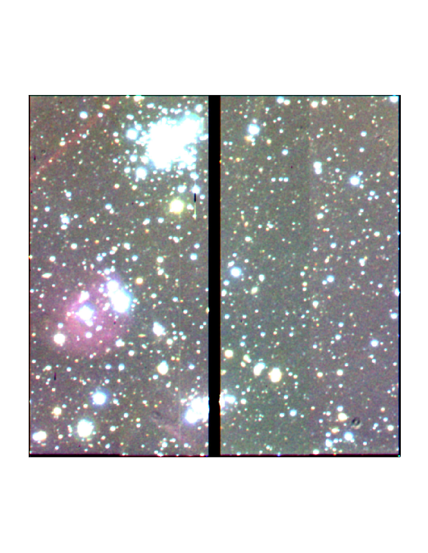
Figure 1: Composite BVR image of BS 216, centred on the left CCD. NGC 796 (above) and WG 8 (below) are also included. North to the top and East to the left.

Photometric standards (Sharpee et al. 2002) were observed each night at different airmasses. In the nights of January 16th and 17th, 2010, however, the latter fields were too high. We then used standards in the SN 1987A neighbourhood (Walker & Suntzeff 1990). Exposure times for the standards varied in order to allow high S/N measurements over the full range of standard mags. From 30 to 50 bias frames were taken by the SOAR resident astronomers prior to each observing run. In addition, 20 dome flat images were taken with the 3 filters, except for the last two nights, when 15 dome flats were taken. Typical counts per flat exposure were 16-18K for B, 17-22K for V, and 18-20K for R. The data reductions were carried out within IRAF, using the mscred and soar packages. For each night, a single coadded image was created from each set of the run bias and flat exposures. Extreme points in the distribution of count values were eliminated and the median count value from the remaining frames was stored in the coadded calibration images. These were then visually inspected and had their noise statistics cross examined to those of individual exposures. Science images were then processed. All exposures, including the bias and flat coadds, were first trimmed according to the TRIMSEC parameter in the header. The overscan region of each CCD controller (BIASEC parameter) was fitted with a cubic spline and the resulting count level at each column was subtracted from the exposed areas. This was done for the science exposures and calibration images. The residual bias image was then subtracted from the science exposures and flats. Finally, the exposures were divided by the resulting flat images in each filter, in order to account for non-uniform pixel sensitivity. The exposures were then separated according to on-cluster or off-cluster, filter and exposure time and then coadded. A median filtering was used. The offsets among the exposures to be combined were measured in an automated way, by finding the offset value in CCD positions that maximized the number of matched bright stars in each exposure relative to the first one in the list.

2.1 Calibration

The photometric standards were identified in each exposure, also using an automatic finder. It runs a basic astrometry using the pixel scale and header parameters and then tries to maximize the number of stars from the list of standards, given a positional tolerance. Measurements on these standards were also made automatically using a 5 pixel aperture. The IRAF digiphot task PHOT was used. A PSF model was built on each of the standard exposures. The PSF candidates were pre-selected in each standard field (2 from Sharpee et al. 2002 and 1 from SN1987A) and were found using the same approach as in the case of the photometric standards. A circularly symmetric gaussian PSF was fitted to the stars in each exposure. The IRAF digiphot PSF task was used for this purpose. A calibration equation of the form

$$m=\mu+A\times colour+B\times X+C$$ (1)

was fitted in separate for each night using the standards, where $m$ is the intrinsic mag in the Johnson-Cousins system, $\mu$ is the instrumental mag, colour is the standard colour in B-V, $X$ is the airmass, and $A,B$, and $C$ are fitting coefficients. In order to prevent low S/N measurements and saturated stars from contaminating the calibration, a $2\sigma$ clipping criterion (Table 1) to the list of calibrating stars was applied iteratively until convergence.

Table 1: Log of observations

Date	Band	N	$\sigma$	Target
2009-12-17	B	29	0.068	BS 216, NGC 796, WG 8
2009-12-17	V	29	0.060	BS 216, NGC 796, WG 8
2009-12-18	B	31	0.062	WG 11
2009-12-18	V	33	0.138	WG 11
2009-12-26	B	31	0.080	WG 13
2009-12-26	V	33	0.150	WG 13
2010-01-16	B	18	0.028	BS 245
2010-01-16	V	19	0.024	BS 245
2010-01-17	B	22	0.064	BS 240
2010-01-17	V	24	0.120	BS 240
2010-08-30	B	21	0.056	BS 223
2010-08-30	V	18	0.023	BS 223
2010-09-10	B	23	0.090	BS 226, BS 225, WG 15
2010-09-10	V	22	0.035	BS 226, BS 225, WG 15
2010-09-30	B	15	0.023	BS 232
2010-09-30	V	21	0.050	BS 232
2010-10-01	B	27	0.047	BS 235, BS 233
2010-10-01	V	29	0.103	BS 235, BS 233
2010-10-17	B	18	0.045	BS 239
2010-10-17	V	20	0.085	BS 239
2010-11-13	B	29	0.184	BBDS 4
2010-11-13	V	32	0.131	BBDS 4

• N is the number of standard star measurements; $\sigma$ for clipping criterion

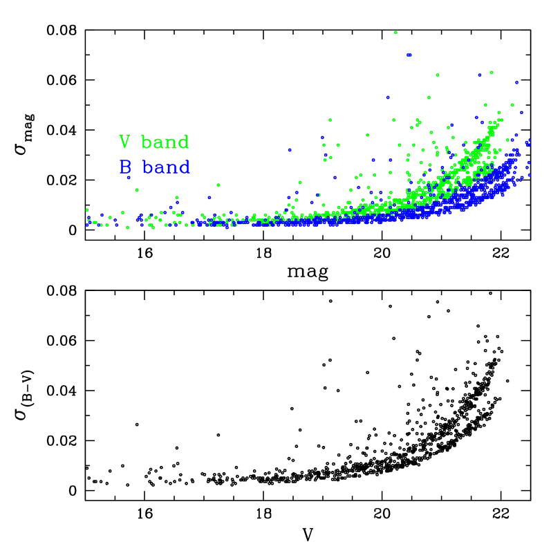
Figure 2: Photometric uncertainties in V and B magnitudes (upper panel) and in (B-V) colour (lower panel

for NGC 796.

Similarly, the IRAF digiphot package was used to source detection and photometry in the on-cluster and off-cluster coadds. A threshold of 5 times the sky fluctuation was used for source detection on the V band coadds. This source table was used to perform aperture photometry in the B and V filters. The mean FWHM in each coadd was used for aperture photometry. A circularly symmetric Gaussian PSF model was also built on each on-cluster and off-cluster coadds. In each image the PSFs of the 40 brightest unsaturated stars were visually inspected in order to select the best ones to build the PSF models. The ALLSTAR task was used to compute x and y centres, sky values, and mags. performing fits of the PSF models to groups of stars in each coadd. Parameters as the fitting and PSF radii were taken based on the mean FWHM for each image, as described in the DAOPHOT manual. Each star center was recomputed in every fit iteration, and so was the sky value, considered as a single value for each group of stars in the fitting. The calibration equation for each night was then applied to the science fields. The calibrated magnitude and intrinsic colours were computed simultaneously for each star. The instrumental colour was used as an initial guess in the calibration equation, yielding an initial value of the calibrated magnitude. A new colour was then computed and the process reiterated until all colours converged to 0.01 mag. Uncertainties in the calibrated magnitudes were derived by propagating the uncertainties in the instrumental magnitudes, and calibration parameters. In order to illustrate these values, we present the final uncertainties in magnitudes and colour for NGC 796 in Fig. 2.

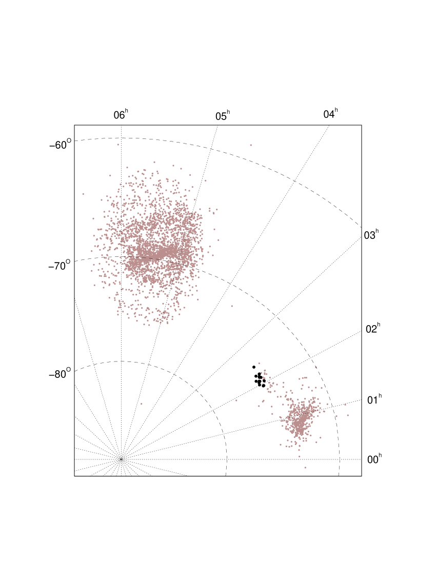
Figure 3: Location of the sample clusters and associations (black points) with respect to the LMC and SMC cluster positions in the catalogue by (Bica et al., 2008)).

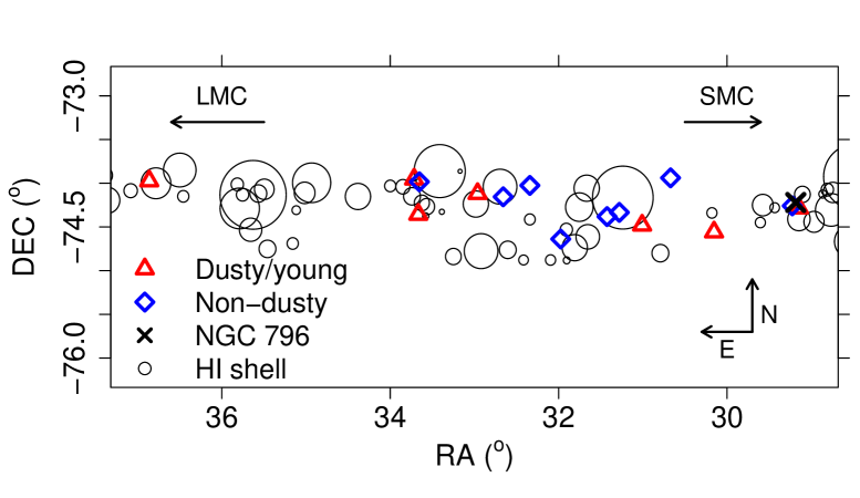
Figure 4: Location of the sample clusters and H I shells with respect to the LMC and SMC, where the data points are from Bica et al. (2008). North to the top and East to the left.

3 General properties of the sample objects

Fourteen star clusters and two associations could be extracted from the SOAR images, as shown in Table 3, for which the density classes (C, A, AC, CA) are from Bica & Schmitt (1995). The acronyms in Table 3 are L58 (Lindsay 1958), L61 (Lindsay 1961), WG(Westerlund & Glaspey 1971), ESO (Lauberts 1982), ICA (Battinelli & Demers 1992), BS (Bica & Schmitt 1995), BBDS (Bica et al. 2008).

We show in Fig. 3 the positions of the present sample clusters with respect to the overall clusters in the Bica et al. (2008), which traces the present structure with respect to the Bridge, LMC and SMC.

In Fig. 4 the present clusters are shown in the corresponding Magellanic Bridge sector, together with the H I shells in the area. The directions to both Clouds are shown, as well as our classification of dusty and non-dusty clusters (see Table 3 and Sect. 5). Coordinates and sizes of clusters and H I shells are from Bica et al. (2008) and references therein. Dusty clusters basically correlate angularly with H I shells. Fig. 5 shows a mosaic of BVR images of the objects, built with the present observations. The mosaic shows a range of stellar densities, from extremely compact to loose ones. The clusters BBDS 4 and BS 216 appear to be associated to gas emission in optical images.

The compact cluster WG 15 is projected close to the edge of the association ICA 18. Too few stars could be retrieved by the extraction routine in WG 15, so we analyse the ensemble of ICA 18, including WG 15.

We indicate in Table 2 the foreground reddening values predicted by Schlegel, Finkbeiner & Davis (1998) and Schlafly & Finkbeiner (2001) for the present sample cluster directions, taking three of them for their strategic positions along the Bridge. We indicate the cluster values closer to the SMC Wing, farthest away from the SMC in the Bridge, and one third of the way between both.

Table 2: Reddening for objects across the Bridge from HI columns

Cluster	$\alpha$	$\delta$	$A_{V}^{(1)}$	$A_{V}^{(2)}$	Note
	(h:m:s)	(°:′:″)	(mag)	(mag)
(1)	(2)	(3)	(4)	(5)	(6)
BS 216	1:56:54	-74:15:28	0.158	0.131	close to SMC Wing
BS 245	2:27:27	-73:58:23	0.166	0.138	far in the Bridge
BS 233	2:10:38	-74:09:20	0.181	0.222	one third away

• (1): Schlegel, Finkbeiner & Davis (1998); (2): Schlafly & Finkbeiner (2001).

Some sample objects seem to be asymmetric in the stellar distribution, such as BS 216 and especially WG 13, in the sense that there occurs a deficiency of stars in a hemisphere, with respect to the bright central star (Fig. 5). Asymmetry effects do not appear to be an exclusive trait of young Magellanic clusters (see e.g. the Galactic proto-clusters in Camargo, Bonatto & Bica 2011 and Camargo, Bica & Bonatto 2015), but they are rare in large collections of CCD cluster images of the SMC and LMC (Pietrzynski et al. 1998; Pietrzynski et al. 2000). The effect is probably related to star formation and evolution under two sources of tidal stresses. Asymmetrical tidal effects might e.g. preferentially erode the molecular clouds exposing molecular cores, or affect the early dynamical evolution by exposing stellar cores as a consequence of evaporation.

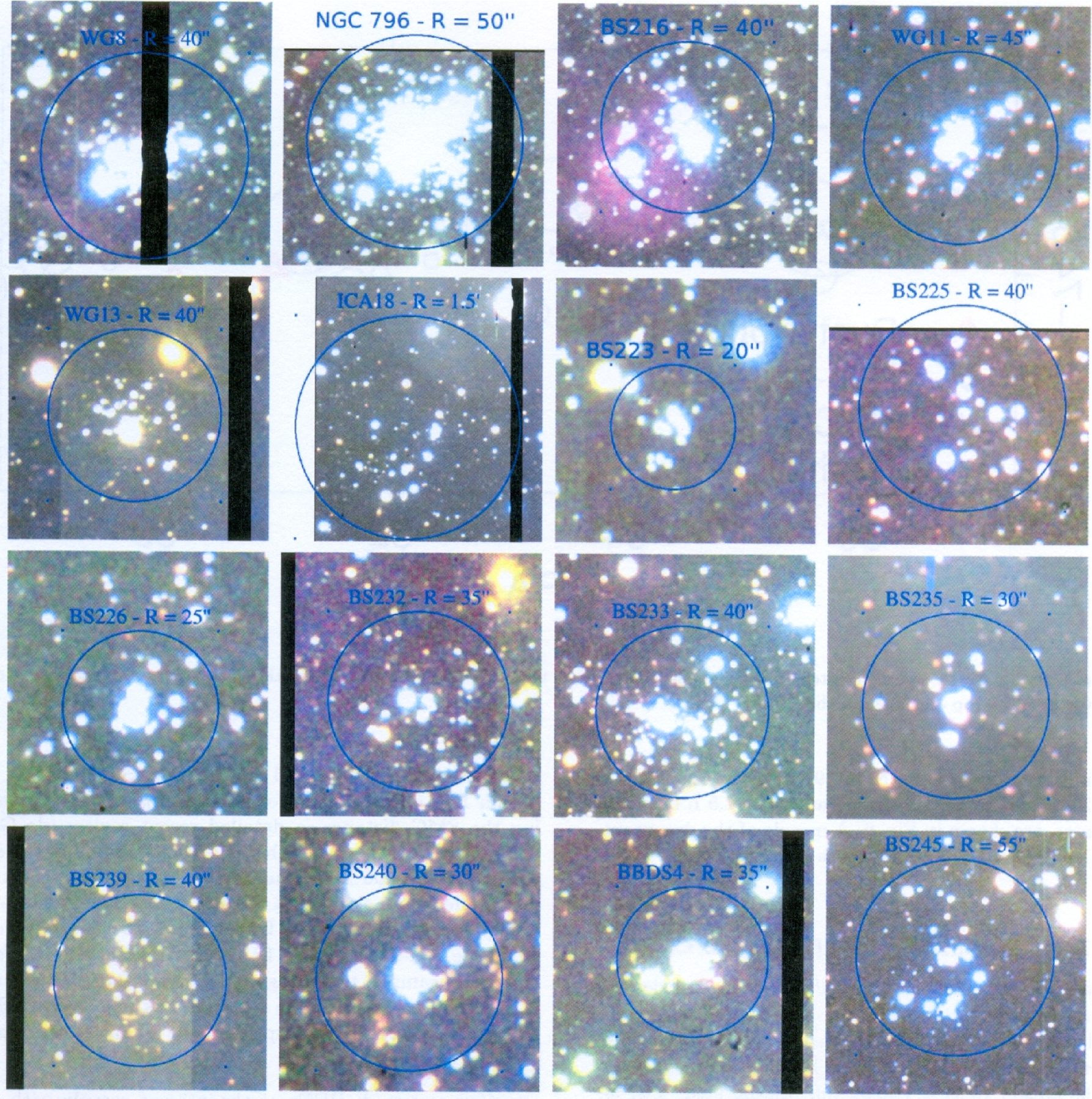
Figure 5: Composite BVR images of the sample targets centred on the coordinates in Table 3. Each panel is $1\times 1\arcmin^{2}$. Circles show the bulk of the cluster stars. North to the top and East to the left.

Table 3: The Bridge sample

Designation	$\alpha$	$\delta$	class	D	d	Part of	Dust
	(h:m:s)	(°:′:″)		(′)	(′)
(1)	(2)	(3)	(4)	(5)	(6)	(7)	(8)
WG 8	1:56:35	-74:17:00	AC	1.00	0.50	in BS 215	Y
NGC 796,L 115,WG 9,ESO 30SC6	1:56:44	-74:13:10	C	1.20	1.10	in BS 215	N
BS 216‡	1:56:54	-74:15:28	C	0.40	0.40	in BS 217	Y
WG 11‡	2:00:37	-74:33:29	C	0.70	0.55		Y
WG 13‡	2:02:41	-73:56:21	C	1.10	0.85		N
ICA 18†‡	2:07:54	-74:38:17	A	3.20	2.30		N
BS 223‡	2:04:02	-74:28:48	C	0.35	0.35	in BS 224	Y
BS 225	2:05:07	-74:20:02	A	1.10	0.75		N
BS 226‡	2:05:42	-74:22:53	C	0.40	0.35	in ICA9	N
BS 232‡	2:09:22	-74:01:31	CA	0.80	0.80	in BS 231	N
BS 233‡	2:10:38	-74:09:20	CA	1.20	1.10	in DEMS169	N
BS 235‡	2:11:51	-74:07:08	C	0.60	0.40		Y
BS 239‡	2:14:37	-73:59:00	CA	1.20	0.65	in ICA 34	N
BS 240‡	2:14:52	-73:57:10	C	0.30	0.30	in BD34	Y
BBDS 4‡	2:14:40	-74:21:24	C	0.30	0.20	in L61-593	Y
BS 245‡	2:27:27	-73:58:23	CA	1.10	0.90	in ICA 44	Y

• $\dagger$ The compact cluster WG 15 (2:07:40, -74:37:45 , C, 0.35′) is located at the edge of association ICA 18. By columns: (1) object designation(s), (2) and (3) J2000.0 equatorial coordinates, (4) density class, (5) and (6) major and minor diameters, (7) part of larger object, in general an association. (8) evidence of embedded cluster from SPITZER and/or WISE dust emission: Y(es) or N(o). Information from Bica et al. (2008) and references therein. $\ddagger$ Cluster centred on the CCD.

Although field star contamination is not critical in the intercloud region, we carried out a statistical field subtraction following Bonatto & Bica (2007). Examples of the decontamination procedure for NGC 796 near the SMC Wing, and BS 245 quite far in the Bridge at $\Delta\alpha$ = 1.5 h from the SMC center, are shown in Fig. 6. A mosaic of the decontaminated CMDs of the whole sample is given in Fig. 8.

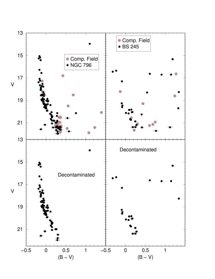
Figure 6: Field-star decontamination examples for NGC 796 and BS 245.

4 Radial density profiles and CMDs

We show in Fig. 7 the resulting mosaic of Radial density profiles (RDPs). The RDPs show in general significant central stellar densities and radial extensions which we measure by means of R_RDP (e.g. Camargo, Bonatto & Bica 2011), where the cluster density equals that of the field. The individual shapes of the profiles indicate core/halo structures immersed on a rather shallow background. For all objects in Table 3 we searched for automated optimized centres with maximum density, within a radius $r=10\arcsec$. The background level and uncertainty are estimated based on the star counts and fluctuation measured on the surrounding area beyond the cluster radius (Fig. 7). Usually, we used all the available area outside the cluster to estimate the background level and perform the field decontamination. Since the projected area of the targets vary and the CCD field of view is fixed, the comparison field changes with every case. However, we point out that, in all cases, the comparison field area is larger than those of the clusters.

Examples are given in Fig. 7, in which we adopted $1\,\sigma$ values for the background uncertainty. This allows to estimate the RDP extent, basically defined as the radius where background and cluster profile meet (e.g. Camargo, Bonatto & Bica (2011)). We illustrate in Fig. 6 the background determination for NGC 796 and BS 245. For NGC 796, we obtain $R_{RDP}\approx 0.8\arcmin$, and for BS 245, $R_{RDP}\approx 1\arcmin$. Regarding the SMC distance, a detailed recent review (de Grijs & Bono 2015) came up with the distance modulus value of $(m-M)_{O}=18.96\pm 0.02$ mag (62 kpc). Note, however, that depth effects are significant (Crowl et al. (2001)). For simplicity, we assume 62 kpc. In this case, the absolute radii would be $\sim 14.4$ pc and $\sim 18$ pc. Considering the RDPs of the whole sample, the Bridge clusters are larger than most of the young clusters in the Galactic disk (e.g. Saurin, Bica & Bonatto 2012). So, they appear to be inflated with respect to Galactic counterparts.

Comparing all RDPs of the present sample with the respective absolute radii of the Galactic star cluster catalogue of Kharchenko et al. (2013) in Fig. 9, it is clear that the Bridge objects occupy the large-radii wing of the distribution. The sample of Kharchenko et al. (2013) contains primarily clusters old enough to be trimmed by the Milky Way tidal field. One possible conclusion is that Bridge clusters are formed as relatively large structures. Note that the present section assumes a SMC distance of 62 kpc. Given that the Bridge connects the SMC with the LMC and that implies a gradient in distance corresponding to a distance modulus variation of at leas 0.5 mag, we also consider the effects on cluster size for a shorter distance of $\sim$ 40 kpc for the Bridge clusters (Sect. 8). They still occupy the large-size wing in Fig. 9.

We propose that the Bridge clusters are inflated as a consequence of tidal fields in their formation and early evolution under the SMC and LMC tidal stresses. Interestingly, clusters with structural asymmetries also present a break towards the core in the RDPs (Fig. 7).

5 NGC 796 and Young CMD templates

As observed in a 4m class telescope, most sample clusters seem to be relatively poorly-populated, but we recall that we are dealing with young Magellanic clusters, so they may be intrinsically more massive. Thus, to mitigate the rather-low statistics, we decided to create templates based on their CMDs. The dusty clusters (Table 3) form a young group with 5 entries: BS 223, BS 235, BS240, BS 245, BBDS 4. Although dusty, BS 240 has not been included in the template because its CMD resulted very poor.

The remaining clusters and associations, ICA 18, BS 239, BS 233, BS 232, WG 13, BS 216, BS 225 and BS 226, are not dusty (Table 3). They all have CMDs very similar to that of NGC 796, which might suggest a coeval star-formation event. All but one of the dusty clusters share their same spatial location on the Bridge with non-dusty clusters (see Fig. 4). The groups are built by applying, when necessary, small shifts in magnitude ($\sim 0.03$) and, to a lesser extent, colour ($\sim 0.01$). The reason for this is to obtain statistically significant CMDs with which to derive parameters such as age, reddening and distance. Then, the individual CMDs can be matched to the respective template ones to derive the individual parameters. At this point, we have 3 populous CMDs suitable for a more detailed analysis (Fig. 10): (i) NGC 796 itself, (ii) a dusty template, and (iii) a dust-free one, very similar to NGC 796.

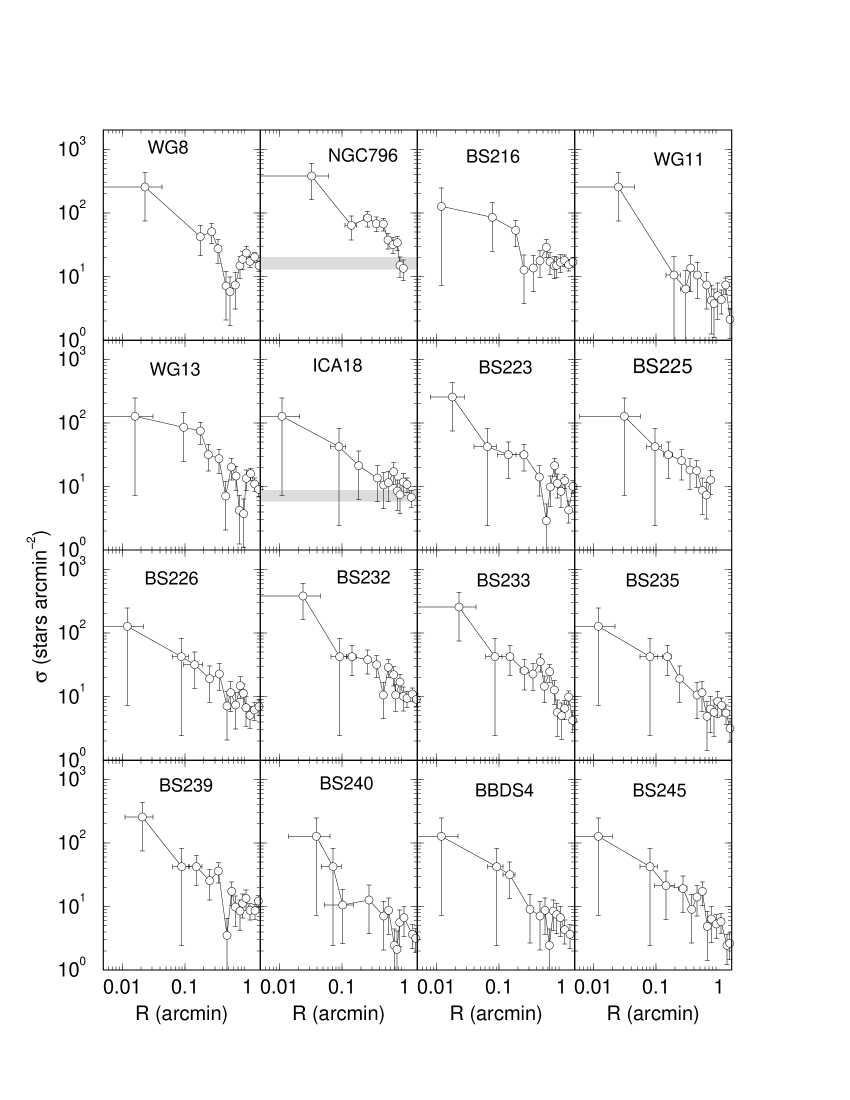
Figure 7: Stellar density distributions of clusters and associations. Grey stripes illustrate background level and uncertainty for NGC 796 and ICA 18.

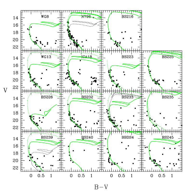
Figure 8: Visual isochrone fittings to the decontaminated CMDs all clusters and associations (green solid lines), except for NGC 796, where a numerical-statistical method was used to find the best solution (see Sect. 6). The physical parameters used for these fits are presented in Table 5. For comparison purposes, the template isochrone fittings (green dotted lines) and the physical solutions proposed by Piatti et al. (2007) (NGC 796) and Piatti et al. (2015) (BS 233, BS 239 and BBDS 4) are also presented (black dotted lines). The size of photometric uncertainties vs. magnitude and colour are illustrated in Fig.2.

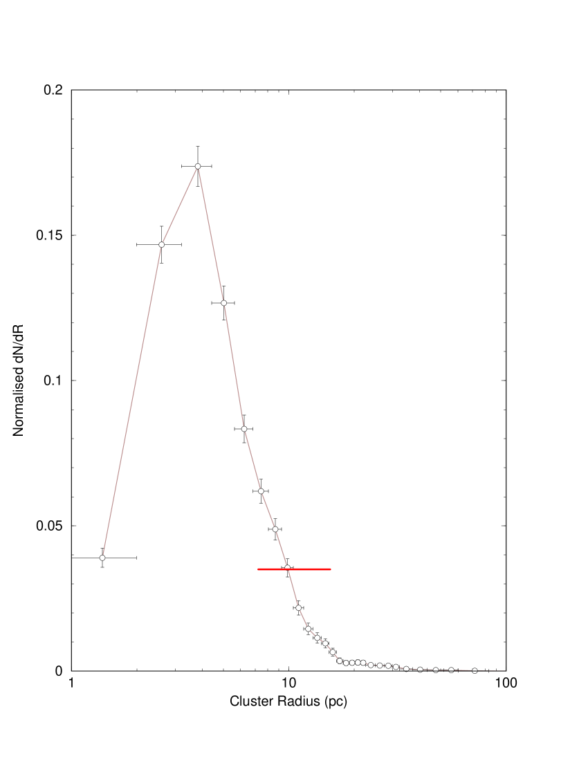
Figure 9: Comparison of the radius of the present sample objects (red) with Galactic star clusters (Kharchenko et al. 2013), assuming a SMC distance modulus of 62 kpc (de Grijs & Bono 2015).

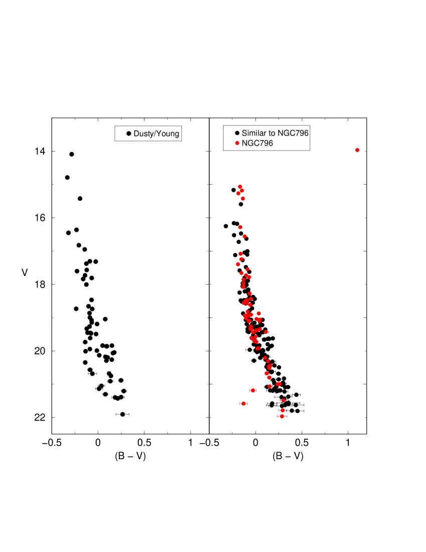
Figure 10: Photometric templates. Left: dusty CMDs. Right: dust-free CMDs compared to the populous NGC 796.

6 Method of analysis

In order to recover the age, metallicity, distance modulus and reddening for NGC 796 and for the two templates we applied a numerical-statistical isochrone fitting. This method was initially developed to derive physical parameters for LMC clusters observed with HST (Kerber et al., 2002; Kerber & Santiago, 2005; Kerber, Santiago & Brocato, 2007), but more recently it was used to analyse open clusters in the near-infrared (Alves et al., 2012) and SMC clusters observed with SOAR under very similar conditions with respect to the data presented here (Dias et al., 2014). In short, it is based on objective comparisons between observed CMDs and synthetic ones using a likelihood statistics. Those models that maximize this statistics are identified as the best ones, and then they are used to constrain the stellar cluster physical parameters. Fig. 11 illustrates the generation of a synthetic CMD that was compared with the observed CMDs in this work. Essentially the probability of a star to belong to a specific model is measured by the density of points in its CMD. So the likelihood of this model will be proportional to the product of these probabilities for the observed stars.

To avoid local or biased solutions we have explored a wide range of values and a regular grid of models in the space parameter, virtually rising all possible solutions that can be considered among the best ones. Typically we use $\sim 10^{4}$ combinations in log($\tau$/yr), $Z$, $(m-M)_{0}$ and $E(B-V)$ centred in an initial guess obtained by a visual isochrone fit. In terms of distance modulus, we investigated solutions from 17.70 to 19.30, by far covering the most acceptable results for the SMC distances and its complex geometry (de Grijs & Bono, 2015), including the large line-of-sight depth for the SMC eastern side ($\sim 23$ kpc) recently found by Nidever et al. (2013). Concerning the age, metallicity and reddening, we searched for solutions in the following ranges: $6.60<$ log($\tau$/yr)$<10.00$ (steps of 0.05); $0.0001<$ Z $<0.0020$ (steps of $\sim$ 0.002); $0.00<$ $E(B-V)$ $<0.30$ (steps of 0.01). Once again, these ranges are sufficiently wide to cover any result concerning the SMC or the Bridge, like the ones present in the SMC age-metallicity determinations for stellar clusters (Piatti, 2011; Parisi et al., 2014) and field stellar populations (Carrera et al., 2008; Rubele et al., 2015), in the analysis of Bridge field stars (Nidever et al., 2013; Skowron et al., 2014), and reddening maps (Burstein & Heiles, 1982; Schlegel, Finkbeiner & Davis, 1998).

Since the uncertainties in the physical parameters are computed using synthetic CMDs that are reproducing the observed ones, the spread of stars and the stochastic effect due to the photometric uncertainties and the limit number of observed stars are naturally incorporated in our results. For further details we recommend the reader to consult the aforementioned works.

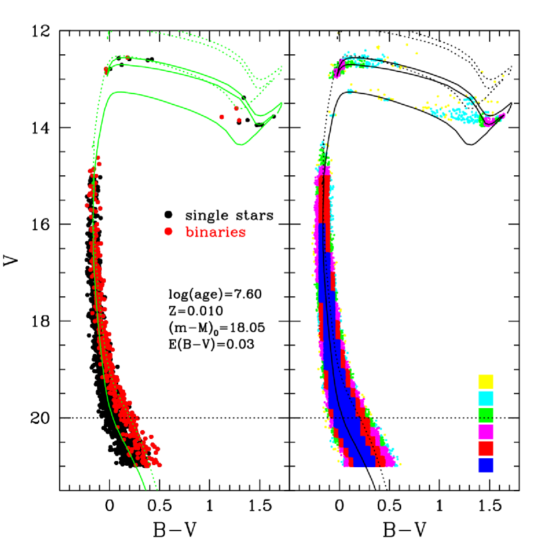
Figure 11: Generation of synthetic CMDs. Left: an example of synthetic CMD generated with 2000 stars. The adopted isochrone (green solid line) and its physical parameters are presented in the panel. Right: the same as in the left panel, but for 10000 stars. The colours in this case are following the density of points, which means the probability to generate stars in that CMD position. The isochrone for equal mass binaries is also shown in both panels (dotted lines). We adopted a power-law mass function following the Salpeter slope and a binary fraction of 30%.

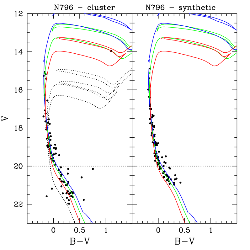
Figure 12: Best isochrone fittings for NGC 796. Left panel: observed stars and three isochrones with the parameters found in Table 4. The different solid lines correspond to the central solution (green), the young/metal-rich solution (blue) and the old/metal-poor solution (red). The physical solution proposed by Piatti et al. (2007) is also presented (dotted line). Right panel: synthetic CMD generated with the parameters found for the best solution.

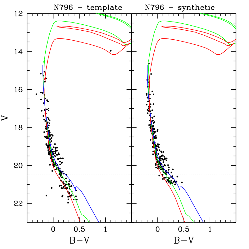
Figure 13: The same as in Fig. 12 but for the NGC 796 template.

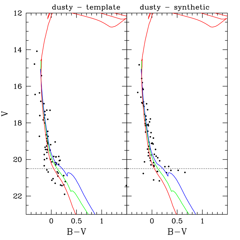
Figure 14: The same as in Fig. 12 but for the dusty/young template.

Table 4: Self-consistent physical parameters derived by us using our numerical-statistical isochrone fitting.

Name	log($\tau/yr$)	Age(Myr)	Z	[Fe/H]	(m-M)0	d(kpc)	E(B-V)
NGC 796	$7.63\pm 0.19$	$42^{+24}_{-15}$	$0.010\pm 0.005$	$-0.3^{+0.2}_{-0.3}$	$18.04\pm 0.28$	$40.6\pm 1.1$	$0.03\pm 0.02$
NGC 796 - template	$7.41\pm 0.24$	$25^{+18}_{-11}$	$0.010\pm 0.005$	$-0.3^{+0.2}_{-0.3}$	$18.01\pm 0.26$	$40.1\pm 1.1$	$0.04\pm 0.02$
Dusty - template	$7.22\pm 0.14$	$16^{+6}_{-5}$	$0.006\pm 0.004$	$-0.5^{+0.2}_{-0.5}$	$17.96\pm 0.26$	$39.2\pm 1.1$	$0.04\pm 0.03$

7 Results

Based on the results of the previous sections, we use the CMD templates to estimate parameters for individual clusters by computing magnitude and colour differences with respect to the templates (including NGC 796).

Table 5 reports physical parameters derived by a visual isochrone fitting method, as shown in Fig. 8. The uncertainties presented in this table correspond to the range of acceptable solutions based on a visual inspection. Certainly these values are conservative, and they can be used as an upper limit. On the other hand, a lower limit for the uncertainties in these determinations can be found in Table 4, where the random uncertainties for the numerical-statistical method are presented.

Almost all clusters have ages from log(age)=7.30 (BBDS 4) to log(age)=8.30 (BS 233). The only exception is BS 226, the oldest cluster in our sample (log(age)=8.95). Another interesting result is related to the the distance determinations: all clusters are located at distance modulus between 17.95 (BBDS 4) and 18.40 (WG 13 and BS 233), therefore even closer than the canonical LMC value of $(m-M)_{0}=18.50$ mag (de Grijs, Wicker & Bono, 2014).

We have NGC 796 in common with Piatti et al. (2007) (Washington photometry with ESO 1.54 Danish telescope) and BS 226, BS 232, BS 233, BS 235, BS 239, BS 240 and BBDS 4 in common with Piatti et al. (2015) (Near-infrared photometry with VISTA). A comparison with their results leads to the following conclusions.

Piatti et al. (2015) imposes a metallicity of Z=0.003, and a distance modulus of $(m-M)_{0}$ = 18.90 mag, and adopted the E(B-V) values from several sources. The age is then derived from visual isochrones fittings to the CMDs. We instead fit all parameters, such that differences are pointed out below.

NGC 796

A comparison of the present fit for NGC 796 (L115) and that by Piatti et al. (2007) is shown in Figs. 12 and 13. They derived visually an age of log(age)=8.05-8.20 for NGC 796, assuming that it is at a distance modulus of $(m-M)_{0}$ = 18.77, a metallicity of Z=0.003 and a reddening E(B-V)=0.03, from maps by Burstein & Heiles (1982) and Schlegel, Finkbeiner & Davis (1998). It is clear that the solution by Piatti et al. (2007) does not fit the brightest stars of the cluster (their fit corresponds to the dotted lines). An inspection of data used by Piatti et al. (2007) indicates that the images used were saturated for the bright stars, and no short exposures are mentioned. Therefore we are confident that NGC 796 is younger than reported by Piatti et al. (2007), with an age of log(age)$\sim 7.6$, and that it is located at a short distance ($(m-M)_{0}\sim 18.04$, $d\sim 41$ kpc).

BS 226, BS 232, BS 235 and BS 240 Piatti et al. (2015) classify these cluster as “possible non-cluster” or “not recognized”. However, our deeper photometry indicates them as clusters, especially for the main sequence distributions shown in Fig. 8 for BS 226 and BS 232. The remaining two have less-populated main sequences.

BS 233 For BS 233 Piatti et al. (2015) report an age of log(age)=7.3 yr, having assumed a reddening of E(B-V)=0.15, and a distance modulus of $(m-M)_{0}=18.90$, and metallicity Z=0.003, whereas the present results give E(B-V)=0.0 and log(age)=8.3 yr, together with a metallicity of Z=0.001. Figure 8 shows that the present solution fits the data more satisfactorily.

BS 239 Fig. 8 shows that the present results of E(B-V)=0.04, Z=0.010 and log(age/yr)=8.0 fit better the data than the Piatti et al. (2015) solution of E(B-V)=0.11, Z=0.003 and log(age/yr)=8.5.

BBDS 4 Fig. 8 shows that both solutions from the present work of E(B-V)=0.01, Z=0.004 and log(age/yr)=7.3 and those from the Piatti et al. (2015) solution of E(B-V)=0.08, Z=0.003 and log(age/yr)=9.1 fit the data reasonably well. This cluster is clearly embedded in an H II region.

BS 245 Fig. 8 shows some spread, but a main sequence seems to be confirmed.

Table 5: Physical parameters (and uncertainties) derived by us using visual isochrone fits.

Name	log($\tau/yr$)	Z	(m-M)0	E(B-V)
WG 8	$8.10\pm 0.25$	$0.010\pm 0.006$	$18.30\pm 0.30$	$0.05\pm 0.04$
BS 216	$7.60\pm 0.30$	$0.010\pm 0.006$	$18.00\pm 0.30$	$0.04\pm 0.04$
WG 13	$8.10\pm 0.25$	$0.010\pm 0.006$	$18.40\pm 0.30$	$0.05\pm 0.04$
ICA 18	$7.80\pm 0.30$	$0.010\pm 0.006$	$18.20\pm 0.30$	$0.02\pm 0.02$
BS 223	$8.20\pm 0.25$	$0.008\pm 0.004$	$18.40\pm 0.25$	$0.05\pm 0.04$
BS 225	$7.50\pm 0.30$	$0.010\pm 0.006$	$18.00\pm 0.30$	$0.04\pm 0.04$
BS 226	$8.95\pm 0.15$	$0.002^{+0.002}_{-0.001}$	$18.00\pm 0.20$	$0.04\pm 0.04$
BS 232	$7.90\pm 0.30$	$0.008\pm 0.006$	$18.20\pm 0.30$	$0.05\pm 0.04$
BS 233	$8.30\pm 0.20$	$0.001^{+0.001}_{-0.0006}$	$18.00\pm 0.25$	$0.00^{+0.02}_{-0.00}$
BS 235	$7.40\pm 0.30$	$0.002^{+0.002}_{-0.001}$	$18.20\pm 0.30$	$0.00^{+0.02}_{-0.00}$
BS 239	$8.00\pm 0.25$	$0.010\pm 0.006$	$18.00\pm 0.30$	$0.04\pm 0.04$
BS 240	$8.00\pm 0.25$	$0.010\pm 0.006$	$18.00\pm 0.30$	$0.04\pm 0.04$
BBDS 4	$7.30\pm 0.30$	$0.004^{+0.004}_{-0.003}$	$17.95\pm 0.30$	$0.01^{+0.02}_{-0.00}$
BS 245	$8.00\pm 0.25$	$0.008\pm 0.006$	$18.00\pm 0.30$	$0.01^{+0.02}_{-0.00}$

A comparison of parameters in Table 5 (considering the uncertainties) with the recent values by Piatti et al. (2015) shows the following: (i) a non-negligible difference concerning E(B-V), with ours consistent with the external values quoted in Table 2; (ii) (ii) regarding ages, Piatti et al. (2015) give a younger value for BS 233, but older values for BS 239 and, more significantly, for BBDS 4. Although their solution do not fit well the red main sequence stars in our CMDs, the discrepancies in age for these last two clusters can be partially explained by the absence of the brightest main sequence stars in their CMD analysis; (iii) the metallicities are comparable.

8 Discussions

The present work shows evidence that the Bridge clusters have sizes probably modulated at birth by tidal forces of the LMC and SMC. The present sample is projected in the sky nearer to the less-massive SMC galaxy, as indicated by the centroids of the LMC $\alpha=05^{h}31^{m}00^{s}$, $\delta=-69\degr 22\arcmin 48\arcsec$ and SMC $\alpha=00^{h}53^{m}29^{s}$, $\delta=-73\degr 07\arcmin 48\arcsec$ (Bica et al. 2008), and the present sample coordinates in Table 3.

Compared to a diagnostic-diagram of dynamical evolution for young Galactic clusters (Bonatto & Bica 2010; Saurin, Bica & Bonatto 2012), the present Bridge clusters (and the two associations) have sizes larger than the bulk of embedded clusters in the Galaxy. However, they are considerably smaller than Trumpler 37 and Bochum 1, which have already evolved into associations.

Figure 15: Age histogram for the sample. Note that age uncertainties (Table 5) are smaller than the bin widths.

In the last decades much work has been done on depth effects of the SMC. Crowl et al. (2001) used 12 intermediate age and old star clusters to find a triaxial distribution of 1:2:4 ($\alpha$:$\delta$:depth), with SMC depth effects from 6 to 12 kpc. The 21 cm HI line surveys showed that the SMC, and especially the Wing, appear to be split into two velocity components (e.g. Mathewson 1984; Mathewson, Ford & Visvanathan 1986), with counterparts in Cepheid velocities. The SMC would be splitted into a Mini-Magellanic Cloud and the SMC Remnant, as a consequence of the interactions with the LMC (e.g. Murai & Fujimoto 1980; Mathewson, Ford & Visvanathan 1986; Gardiner & Hawkins 1991). Although these studies propose that the SMC would extend beyond its tidal radius, based on Cepheids in the infrared, Welch et al. (1987) claimed that the SMC should be essentially contained in its tidal radius.

We remark that the distance results are a key issue. The present clusters appear to lie at a distance of $\sim 40$ kpc, thus $\sim 20$ kpc closer than the SMC and $\sim 10$ kpc than the LMC. These results would not fit the scenario where the Bridge is a simple connection between both Clouds, as implied by models like in Besla et al. (2012). Thus, our work discloses the presence of a foreground structure that is projected near the edge of the SMC wing. We conclude that the Bridge, having arisen in the far side of the LMC (Demers et al. 1991), may be indeed a tidal arm. Recently, Subramanian & Subramaniam (2015) studied the SMC structures reaching the Bridge as well by means of Cepheids. Among the results, they find that Cepheids occur in front of the SMC tilted plane. Nidever et al. (2013) found evidence that the stellar component detected at $\sim 55$ kpc is a tidally stripped component from the SMC 200 Myr ago following a close encounter with the LMC.

A deeper insight on the Bridge formation, structure and evolution requires a deeper understanding of the LMC and SMC interaction history over the last Gyrs, e.g. Bekki & Chiba (2008), Besla et al. (2007), and Kallivayalil et al. (2013).

In addition, one cannot rule out an intermediate-age component in the Bridge. For instance, Bagheri, Cioni & Napiwotzki (2013) found that ages of the RGB and AGB stars in the central Bridge region are likely to range from $\sim 400$ Myr to 5 Gyr, implying that these stars were drawn into the Bridge at the tidal event and did not form in situ. The Bridge may not have been formed only by tidal stripping, but probably involved also more complex phenomena. Figure 15 shows the age histogram from Table 5. Although the small number of objects, there is a clear dominance towards $\log(Age/years)\sim 8.2$. This is a hint to the intrinsic star formation history (SFH) in the Bridge. Interestingly, this peak basically coincides with the last interaction between the LMC and SMC (Bekki & Chiba 2005). We conclude that the SFH in the Bridge may be mixed with older populations, as described above.

From the analysis of HI features, Muller et al. (2004) find complex kinematics inside the Bridge and measure $\overline{V_{LSR}}\approx 170km\,s^{-1}$ in our cluster region. Bruns & Westmeier (2004) found $\overline{V_{LSR}}\approx 270km\,s^{-1}$ for the LMC, $\sim 160\,km\,s^{-1}$ for the SMC, and $\sim 215\,km\,s^{-1}$ for the Bridge. Considering the relative velocity between the South-West objects (present sample) in the Bridge and that of the LMC since the last interaction between the Clouds (Bekki & Chiba, 2005), we obtain a distance difference of $\sim 10$kpc, in agreement with the cluster distances in this work. Thus, the tidal dwarf candidate D 1 (Bica & Schmitt 1995) together with its concentration of clusters and associations are consistent with the observed H I kinematics in the area.

9 Concluding remarks

In the present study we derive reddening, metallicity, age, distance modulus and radial density profiles for 14 star clusters and 2 associations of the LMC-SMC Bridge. All clusters are found to be quite young, with ages $7.3<\log(\tau/yr)<8.3$ (except for BS 226 with $\log(\tau/yr))=8.95$), with reddening in the range $0.01<E(B-V)<0.05$ mag. Their metallicities vary in the range $0.001<Z<0.010$, basically encompassing the values previously found for the young populations in the SMC and LMC. Regarding reddening, we recall that the total-to-selective absorption in the SMC indicates R = 2.7, lower than the average Galactic ratio (see e.g. Bouchet et al. (1985)). Although some very young sample clusters have dust emission detected in Spitzer and/or WISE (Table 3), the detected reddening values can be essentially explained from the Galactic foreground (Tables 4 and 5). Consequently, the dust embedding the clusters does not appear to be much effective in absorbing optical light.

Bica & Schmitt (1995) detected 3 probable dwarf galaxies forming along the LMC-SMC Bridge. Differently of the early Universe dwarf galaxies related to stars and dark matter, the ones found by Bica & Schmitt (1995) in the Bridge appear to be tidal products of the latest LMC-SMC interaction. Most of the present clusters are part of the tidal dwarf galaxy candidate D 1, which is associated with an HI overdensity, similarly to D 2 and D 3. Recently, Bechtol et al. (2015) and Koposov et al. (2015) discovered 9 halo dwarf galaxies, part of them projected on the surroundings of the Magellanic Clouds and the Stream. In this context, the young tidal dwarf galaxies populate as well the Lynden-Bell plane (Lynden-Bell, 1976), also called Vast Polar Structure (VPOS), as recently revised and updated by Pawlowski, Pflamm-Altenburg, & Kroupa (2012). However, the conclusive association to such a gigantic structure would require kinematical and orbital data for the newly-found dwarf galaxies (Koposov et al., 2015). Recently, an effort in this direction was the determination of distance and heliocentric velocity of the Reticulum II ultra-faint dwarf galaxy (Simon et al. 2015). However, the transversal velocity is yet needed for a diagnosis. We suggest that the VPOS might as well contain tidal remains of past interactions of the Clouds.

Tidal dwarfs have been detected and described by models (e.g. Mirabel et al. 1992; Barnes & Hernquist 1992), especially for blobs in tidal arms as far as 100kpc from the Antennae. Such tidal dwarf candidates have already been detected in the Bridge connecting the LMC and SMC by Bica & Schmitt (1995) and Bica et al. (2008). Recently, Ploeckinger et al. (2015) (and references therein) presented detailed numerical simulations of the evolution of tidal dwarf galaxies, investigating the decoupling of tidal dwarfs from the tidal arm.

References

- Alves et al. (2012) Alves V.M., Pavani D.B., Kerber L.O. & Bica E., New Astromy, 17, 488
- Bagheri, Cioni & Napiwotzki (2013) Bagheri G., Cioni M.-R. L. & Napiwotzki R. 2013, A&A, 551A, 78
- Barnes & Hernquist (1992) Barnes J.E. & Hernquist L. 1992, Nature 360, 715
- Battinelli & Demers (1992) Battinelli P. & Demers S. 1992, AJ, 104, 1458
- Bechtol et al. (2015) Bechtol K., Drlica-Wagner A., Balbinot E., Pieres A., Simon J.D. et al. 2015, arxiv:1503.02584
- Bekki & Chiba (2005) Bekki K. & Chiba M. 2005, MNRAS, 356, 680
- Bekki & Chiba (2008) Bekki K. & Chiba M. 2008, ApJ, 679, 89
- Besla et al. (2007) Besla G., Kallivayalil N., Hernquist L., Robertson B., Cox T.J., van der Marel R.P. & Alcock C. 2010, ApJ, 721L, 97
- Besla et al. (2012) Besla G., Kallivayalil N., Hernquist L. et al. 2012, MNRAS, 421, 2109
- Bica & Schmitt (1995) Bica E. & Schmitt H.R. 1995, ApJS, 101, 41
- Bica et al. (1999) Bica E., Schmitt H.R., Dutra C.M. & Oliveira H.L. 1999, AJ, 117, 238
- Bica et al. (2008) Bica E., Bonatto C., Dutra C.M. & Santos J F.C. 2008, MNRAS, 389, 678
- Bonatto & Bica (2007) Bonatto C. & Bica E. 2007, MNRAS, 377, 1301
- Bonatto & Bica (2009) Bonatto C. & Bica E. 2009, MNRAS, 394, 2127
- Bonatto & Bica (2010) Bonatto C. & Bica E. 2010, A&A, 516A, 81
- Bouchet et al. (1985) Bouchet P., Lequeux J., Maurice E., Prevot L., Prevot-Burnichon M. L., 1985, A&A, 149, 330
- Bruns & Westmeier (2004) Bruns C. & Westmeier T. 2004, A&A, 426L, 9
- Burstein & Heiles (1982) Burstein D., Heiles C., 1982, AJ, 87, 1165
- Carrera et al. (2008) Carrera R., Gallart C.; Aparicio A., Costa, E., Méndez, R. A.; Noël, N.E.D., 2008, AJ, 136, 1039
- Camargo, Bonatto & Bica (2011) Camargo D., Bonatto C. & Bica E. 2011, MNRAS, 416, 1522
- Camargo, Bica & Bonatto (2013) Camargo D., Bica E. & Bonatto C. 2013, MNRAS, 432, 3349
- Camargo, Bica & Bonatto (2015) Camargo D., Bica E. & Bonatto C. 2015, NewA, 34, 84
- Cioni et al. (2011) Cioni M.-R. L., et al., 2011, A&A, 527, AA116
- Crowl et al. (2001) Crowl H.H., Sarajedini A., Piatti A.E., Geisler D., Bica E., Clariá J.J. & Santos J.F.C. Jr. 2001, AJ, 122, 220
- de Grijs, Wicker & Bono (2014) de Grijs R., Wicker J.E., Bono G. 2014, AJ, 147, 122
- de Grijs & Bono (2015) de Grijs R. Bono G. 2015, AJ, 149, 179
- Demers et al. (1991) Demers S., Grondin L., Irwin M.J. & Kunkel W.E. 1991, AJ, 911, 1114
- Demers & Battinelli (1998) Demers S. & Battinelli P. 1998, AJ, 115, 154
- Dias et al. (2014) Dias B., Kerber L., Barbuy B., Santiago B., Ortolani S. & Balbinot E. 2014, A&A, 561A, 106
- Gardiner & Hawkins (1991) Gardiner L.T. & Hawkins M.R.S. 1991, MNRAS, 251, 174
- Girardi, Bertelli & Bressan (2002) Girardi L., Bertelli G. & Bressan A., Chiosi C., Groenewegen M.A.T., Marigo P., Salasnich B. & Weiss A. 2002, A&A, 391, 195
- Grondin et al. (1990) Grondin L., Demers S., Kunkel W.E. & Irwin M.J. 1990, AJ, 100, 663
- Hodge (1986) Hodge P. 1986, PASP, 98, 1113
- Hodge (1988) Hodge P. 1988, PASP, 100, 1051
- Irwin, Demers & Kunkel (1990) Irwin M.J., Demers S. & Kunkel W.E. 1990, AJ, 99, 191
- Kaallivayalil et al. (2013) Kaallivayalil N., Van der Marel R.P., Besla G., Anderson J. & Alcock C. 2013, ApJ, 764, 161
- Kallivayalil et al. (2013) Kallivayalil N., van der Marel R.P., Alcock C., Axelrod T., Cook K.H., Drake A.J. & Geha M. 2013, ApJ, 764, 161
- Kerber et al. (2002) Kerber L.O., Santiago B.X., Castro R. & Valls-Gabaud D., A&A, 390, 121
- Kerber & Santiago (2005) Kerber L.O. & Santiago B.X., A&A, 435, 77
- Kerber, Santiago & Brocato (2007) Kerber L.O., Santiago B.X. & Brocato E. A&A, 462, 139
- Kharchenko et al. (2013) Kharchenko N.V., Piskunov A.E., Schilbach E., Röser S. & Scholz R.-D. 2013, A&A, 558A, 53
- Koposov et al. (2015) Koposov S.E., Belokurov V., Torrealba G. & Wyn Evans N. 2015, arxiv:1503.02079
- Lauberts (1982) Lauberts A. 1982, ESO/Uppsala survey of the ESO(B) atlas, European Southern Observatory, Garching
- Lindsay (1958) Lindsay E.M. 1958, MNRAS, 118, 172
- Lindsay (1961) Lindsay E.M. 1961, AJ, 66, 169
- Lynden-Bell (1976) Lynden-Bell D., 1976, MNRAS, 174, 695
- Marconi & Clementini (2005) Marconi M. & Clementini G. 2005, AJ, 129, 2257
- Mathewson (1984) Mathewson D.S. 1984, Mercury, 13, 57
- Mathewson, Ford & Visvanathan (1986) Mathewson D.S., Ford V.L. & Visvanathan N. 1988, ApJ, 333, 617
- Mathewson, Ford & Visvanathan (1986) Mathewson D.S., Ford V.L. & Visvanathan N. 1986, ApJ, 301, 664
- McGee & Milton (1966) McGee R.X. & Milton J.A. 1966, AuJPh, 19, 343
- Meaburn (1986) Meaburn J. 1986, MNRAS, 223, 317
- Mirabel, Dottori & Lutz (1992) Mirabel I.F., Dottori H. & Lutz D. 1992, A&A, 256, 19
- Murai & Fujimoto (1980) Murai T. & Fujimoto M. 1980, 32, 581
- Muller et al. (2004) Muller E., Stanimirović S., Rosolowsky E. & Staveley-Smith L. 2004, ApJ, 616, 845
- Nidever et al. (2013) Nidever D. L., Monachesi A., Bell E. F., Majewski S. R., Muñoz R. R., Beaton R. L., 2013, ApJ, 779, 145
- Parisi et al. (2014) Parisi M. C., Geisler D., Clariá J. J., Villanova S., Marcionni N., Sarajedini A., Grocholski A. J., 2014, AJ, 149, 154
- Pawlowski, Pflamm-Altenburg, & Kroupa (2012) Pawlowski M. S., Pflamm-Altenburg J., Kroupa P., 2012, MNRAS, 423, 1109
- Piatti et al. (2007) Piatti A.E., Sarajedini A., Geisler D., Gallart C. & Wischnjewsky M. 2007, MNRAS, 382, 1203
- Piatti et al. (2009) Piatti A.E., Geisler D., Sarajedini A. & Gallart C. 2009, A&A, 501, 585
- Piatti (2011) Piatti A.E., 2011, MNRAS, 418, L69
- Piatti et al. (2015) Piatti A.E., de Grijs R., Rubele S., Cioni M.R., Ripepi V. & Kerber, L. 2015, MNRAS, 450, 552
- Pietrzynski et al. (1998) Pietrzynski G., Udalski A., Kubiak M., Szymanski M., Wozniak P. & Zebrun K. 1998, AcA, 48, 175
- Pietrzynski et al. (2000) Pietrzynski G., Udalski A., Kubiak M., Szymanski M., Wozniak P. & Zebrun K. 2000, Catp005004903, J/AcA/49/521, OGLE LMC star clusters BVI photometry
- Ploeckinger et al. (2015) Ploeckinger S., Recchi S., Hensler G. & Kroupa P. 2015, IAUS, 309, 157
- Rubele et al. (2015) Rubele, S., Girardi, L., Kerber, L., Piatti A.E., Cioni M.R., et al., 2015, MNRAS, 449, 639
- Saurin, Bica & Bonatto (2012) Saurin T.A., Bica E. & Bonatto C. 2010, MNRAS, 407, 133
- Saurin, Bica & Bonatto (2012) Saurin T.A., Bica E. & Bonatto C. 2012, MNRAS, 421, 3206
- Schlafly & Finkbeiner (2001) Schlafly E.F. & Finkbeiner D.P. 2011, ApJ, 737, 103
- Schlegel, Finkbeiner & Davis (1998) Schlegel D.J., Finkbeiner D.P. & Davis M. 1998, ApJ, 500, 525
- Sharpee et al. (2002) Sharpee B., Stark M., Pritzl B., Smith H., Silbermann N., Wilhelm R. & Walker A. 2002, AJ, 123, 3216
- Simon et al. (2015) Simon J.D., Drlica-Wagner A., Li T.S. et al. 2015, ApJ (arXiv:2015.150402889)
- Skowron et al. (2014) Skowron D. M., Jacyszyn A. M., Udalski A., Szymański M. K., Skowron J., et al., 2014, ApJ, 795, 108
- Subramanian & Subramaniam (2015) Subramanian S. & Subramaniam A. 2015, A&A, 573A, 135
- Walker & Suntzeff (1990) Walker A.& Suntzeff N. 1990, PASP, 102, 133
- van den Bergh (1990)
- Welch et al. (1987) Welch D.L., McLaren R.A., Madore B.F. & McAlary, C.W. 1987, ApJ, 321, 162
- Westerlund (1990) Westerlund B.E. 1990, A&ARv, 2, 29