Counterpart synchronization of duplex networks with delayed nodes and noise perturbation

Abstract

In the real world, many complex systems are represented not by single networks but rather by sets of interdependent ones. In these specific networks, nodes in one network mutually interact with nodes in other networks. This paper focuses on a simple representative case of two-layer networks (the so-called duplex networks) with unidirectional inter-layer couplings. That is, each node in one network depends on a counterpart in the other network. Accordingly, the former network is called the response layer and the latter network is the drive layer. Specifically, synchronization between each node in the drive layer and its counterpart in the response layer  (counterpart synchronization, or CS) of this sort of duplex networks with delayed nodes and noise perturbation is investigated. Based on the LaSalle-type invariance principle, a control technique is proposed and a sufficient condition is developed for realizing counterpart synchronization of duplex networks.Furthermore, two corollaries are derived as special cases. In addition, node dynamics within each layer can be various and topologies of the two layers are not necessarily identical. Therefore, the proposed synchronization method can be applied to a wide range of multiplex networks. Numerical examples are provided to illustrate the feasibility and effectiveness of the results.
Keywords: complex network, duplex, counterpart synchronization, stochastic perturbation

• July 2015

1 Introduction

Complex networks abound in almost every aspect of science and technology. Examples include the Internet, the World Wide Web, social networks, metabolic networks, food webs, networks of citations between papers, among many others  [1, 2, 3]. Synchronization is one of the most common phenomena in nature that interacting nodes can reach a coherent state, and it has been extensively investigated and discussed in the past two decades [4, 5, 6, 7, 8, 9, 10]. For example, Pecora et al. [7] used the master stability function (MSF) approach to analyze the stability of the synchronous state in coupled systems, Huang et al. [8] classified synchronization into five categories based on the MSF approach, Wang and Chen investigated synchronization in small-world networks [9] and scale-free [10] networks.

Many literatures, including the above-mentioned ones, are primarily focused on synchronization within single networks that do not interact with other networks. However, many real-world networks often interact with and depend on each other. For example, people in a society interact with each other via their family relationship, friendship, or formal work-related acquaintanceship [11]. Countries in the global economic system also interact via various international relations. Transportation depends on air traffic networks, railway networks and road traffic networks. Obviously, in describing and dealing with such problems, the multiplex network representation would be more appropriate than the single network. Not surprisingly, multiplex networks have attracted enormous attention in the past few years in various fields of application. For example, Xiong et al. [12] analysed the correlation between the information diffusion process and the opinion evolution process and found obvious interaction between the two processes. Liu et al. [13] investigated preferred degree networks and their interactions, and found dramatically different behaviors between two very similar networks.

Counterpart synchronization describes the individuals in one network behave coherently with their counterparts in other associated networks, so it represents harmonious coexistence of nodes in multiplex networks. This sort of synchronization in a duplex network can also be taken as the so-called outer synchronization between two networks and has attracted wide attention. For example, Wu et al. investigated generalized outer synchronization between two different complex dynamical networks by employing nonlinear control [14]. In particular, this synchronization has been widely applied in topology identification of complex networks. To name just a few, Wu [15] and Zhao et al. [16] employed complete outer synchronization to identify topologies for weighted complex networks, Zhang et al. [17] et al. adopted generalized outer synchronization to recover network structures.

Meanwhile, time delays are unavoidable in complex networks due to finite information processing and propagation speeds. They extensively exist in the real world, such as communication networks, gene regulatory networks, and electrical power grids. Time delays greatly influence behaviors of dynamical systems. Many literatures are focused on synchronization and control of complex networks with coupling delay among different nodes [18, 19].

Noise is another important factor affecting behaviors of dynamical systems, as it is inevitable due to environmental disturbance and uncertainties. Generally, noise is harmful. However, the presence of noise sometimes plays a positive role [20], such as in inducing synchronization [21] and in facilitating topology identification of complex networks [22, 23].

Motivated by above discussions, we investigate CS of duplex networks with delayed nodes and noise perturbation. Based on the LaSalle-type invariance principle for stochastic differential delay equations, we design adaptive controllers to synchronize nodes of the response layer to their counterparts in the drive layer, and put forward some sufficient conditions for guaranteeing CS.

The rest of this paper is organized as follows. Modeling of duplex networks and some preliminaries are introduced in Section 2. Sufficient conditions for CS in duplex networks are presented in Section 3. In Section 4, two numerical examples are provided to illustrate the feasibility and effectiveness of our method. Finally, some conclusions are drawn in Section 5.

Notation: Some necessary notations used throughout the paper are introduced. $\mathbf{x}^{\top}$ (or $\mathbf{A}^{\top}$) denotes the transpose of a vector $\mathbf{x}$ (or a matrix $\mathbf{A}$), $\parallel\mathbf{x}\parallel_{2}$ is the Euclidean-norm of $\mathbf{x}$, $\otimes$ represents the Kronecker product, $\mathbb{R}^{n}$ is the $n$-dimensional real space, $I_{n}\in\mathbb{R}^{n\times n}$ represents an identity matrix of order $n$, $C^{n}[a,b]~{}(a,b\in\mathbb{R},~{}a<b)$ represents the $n-$order continuously differentiable function space in $[a,b]$.

2 Modeling and preliminaries

Consider a duplex network consisting of $\mathbf{N}$ nodes in each layer, as shown in Fig. 1. For convenience, take the upper layer as the drive layer and the lower layer which is dependent on signals from the drive layer as the response layer.

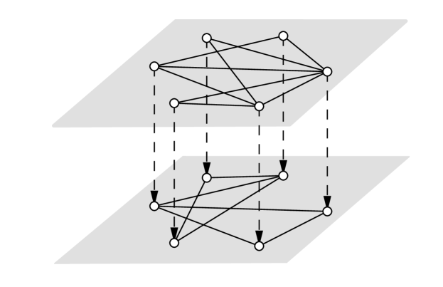
Figure 1: A duplex network with unidirectional inter-layer couplings. Each node in the upper layer is unidirectionally connected to a counterpart in the lower layer. The topologies of the two layers can be different, representing the individual sort of intra-layer interactions.

We are concerned about the impact of delayed nodes and noise caused by control input. Thus a drive layer consisting of $N$ linearly coupled nodes is described by

$$d\mathbf{x}_{i}(t)=[\mathbf{f}_{i}(t,\mathbf{x}_{i}(t),\mathbf{x}_{i}(t-\tau(t)))+\sum_{j=1}^{N}c_{ij}\Gamma\mathbf{x}_{j}(t)]dt,~{}i=1,2,...,N,$$ (1)

and the response layer with control input is given by

$$d\mathbf{y}_{i}(t)=[\mathbf{f}_{i}(t,\mathbf{y}_{i}(t),\mathbf{y}_{i}(t-\tau(t)))+\sum_{j=1}^{N}d_{ij}\Gamma\mathbf{y}_{j}(t)+\mathbf{u}_{i}(t)]dt$$

$$+\mathbf{\sigma}_{i}(t,\mathbf{e}_{i}(t),\mathbf{e}_{i}(t-\tau(t)))d\mathbf{w}(t),~{}i=1,2,...,N.$$ (2)

Here, $\mathbf{x}_{i}(t)=(\mathbf{x}_{i1},...,\mathbf{x}_{in})^{\top}\in\mathbb{R}^{n}$ and $\mathbf{y}_{i}(t)=(\mathbf{y}_{i1},...,\mathbf{y}_{in})^{\top}\in\mathbb{R}^{n}$ are state vectors, $\mathbf{u}_{i}(t)$ is the control input for node $i$, $\mathbf{f}_{i}:\mathbb{R}_{+}\times\mathbb{R}^{n}\times\mathbb{R}^{n}\rightarrow\mathbb{R}^{n}$ is a continuously differentiable function determining the dynamical behavior of node $i$, $\Gamma=(a_{ij})_{n\times n}\in\mathbb{R}^{n\times n}$ is the inner coupling matrix, and $\mathbf{C}=(c_{ij})_{N\times N}\in\mathbb{R}^{N\times N}$ is the coupling configuration matrix representing the coupling strength and the topological structure of network (1), with $c_{ij}$ being defined as follows: if there is a link from node $j$ to node $i~{}(i\neq j)$, $c_{ij}\neq 0$; otherwise, $c_{ij}=0$. The diagonal elements of matrix $\mathbf{C}$ is $c_{ii}=-\sum_{j=1,j\neq i}^{N}c_{ij}$ for $i=1,2,...,N$. $\mathbf{D}=(d_{ij})_{N\times N}\in\mathbb{R}^{N\times N}$ is the coupling configuration matrix of network (2), which has the same meaning as that of $\mathbf{C}$. $\tau(t)$ denotes time delay of nodes, $\mathbf{e}_{i}(t)=\mathbf{y}_{i}(t)-\mathbf{x}_{i}(t)$. The noise term in network (2) is utilized to describe perturbation caused by the control input process influenced by environmental fluctuations [24]. In particular, $\sigma_{i}:\mathbb{R}^{+}\times\mathbb{R}^{n}\times\mathbb{R}^{n}\rightarrow\mathbb{R}^{n\times m}$ is called the noise intensity matrix, $\mathbf{w}(t)=(w_{1}(t),...,w_{m}(t))^{\top}$ is an $m$-dimensional Brownian motion defined on a complete probability space $(\Omega,\mathcal{F},P)$ with a natural filtration $\{\mathcal{F}_{t}\}_{t\geq 0}$.

Throughout this paper, we make the following assumptions:
(H1) The noise intensity function $\mathbf{\sigma}_{i}(t,\mathbf{x},\mathbf{y})~{}(i=1,2,...,N)$ satisfies the Lipschitz condition and there exists positive constants $p,q$ such that

$$trace(\mathbf{\sigma}_{i}^{\top}\mathbf{\sigma}_{i})\leq p\mathbf{x}^{\top}\mathbf{x}+q\mathbf{y}^{\top}\mathbf{y}.$$ (3)

Moreover $\sigma(t,0,0)\equiv 0$.
(H2) There exists a positive constant $M$ such that

$$\|\mathbf{f}_{i}(t,\mathbf{x}_{i}(t),\mathbf{x}_{i}(t-\tau(t)))-\mathbf{f}_{i}(t,\mathbf{y}_{i}(t),\mathbf{y}_{i}(t-\tau(t)))\|$$

$$\leq{M}[\|(\mathbf{x}_{i}(t)-\mathbf{y}_{i}(t))\|^{2}+\|(\mathbf{x}_{i}(t-\tau(t))-\mathbf{y}_{i}(t-\tau(t)))\|^{2}]^{\frac{1}{2}}.$$ (4)

(H3) $\tau(t)$ is a differentiable function with

$$0\leq\dot{\tau}(t)\leq\mu<1.$$ (5)

Obviously, this assumption is ensured if the delay $\tau(t)$ is constant.

Our purpose is to design proper controllers so that the noise-perturbed response layer (2) can reach CS with the drive layer (1). For this purpose, some necessary concepts and a lemma of stochastic differential equations are presented.

Consider the following $n$-dimensional stochastic differential delay equation:

$$d\mathbf{z}(t)=\phi(t,\mathbf{z}(t),\mathbf{z}(t-\tau))dt+\varphi(t,\mathbf{z}(t),\mathbf{z}(t-\tau))d\mathbf{w}$$ (6)

on $t\geq 0$ with an initial value $\xi\in C_{\mathcal{F}_{0}}^{\mu}([-\tau,0],\mathbb{R}^{n})$, where $C_{\mathcal{F}_{0}}^{\mu}([-\tau,0],\mathbb{R}^{n})$ represents the family of all ${\mathcal{F}_{0}-}$measurable bounded $C([-\tau,0],\mathbb{R}^{n})-$valued random variables, the measurable functions $\phi,\varphi:[0,+\infty]\times\mathbb{R}^{n}\times\mathbb{R}^{n}\rightarrow\mathbb{R}^{n}$ satisfy the locally Lipschitz condition and the linear growth condition. It is known that Eq.(6) has a unique solution for any initial value $\xi$ that is denoted by $\mathbf{z}(t,\mathbf{\xi})$ on $t\geq-\tau$.

Let $C^{1,2}(\mathbb{R}_{+}\times\mathbb{R}^{n},\mathbb{R}_{+})$ denote the family of all non-negative functions $V(t,\mathbf{z})$ on $\mathbb{R}_{+}\times\mathbb{R}^{n}$, which are continuously once differentiable in $t$ and twice differentiable in $\mathbf{z}$. For each $V\in C^{1,2}(\mathbb{R}_{+}\times\mathbb{R}^{n},\mathbb{R}_{+})$, the diffusion operator $\mathcal{L}V$ associated to (6) acting on $C^{1,2}(\mathbb{R}_{+}\times\mathbb{R}^{n},\mathbb{R}_{+})$ is defined by

$$\mathcal{L}V=\frac{\partial V}{\partial t}+\frac{\partial V}{\partial z}\cdot\phi+\frac{1}{2}trace[\varphi^{T}\frac{\partial^{2}V}{\partial^{2}z}\cdot\varphi],$$ (7)

where $\partial V/\partial\mathbf{z}=(\partial V/\partial z_{1},...,\partial V/\partial z_{n}),\partial^{2}V/\partial^{2}\mathbf{z}=(\partial^{2}V/\partial z_{i}\partial z_{j})_{n\times n}$.

Lemma 2.1

(A Lasalle-type invariance theorem for stochastic differential equations [25]). Assume that both $\phi(t,\mathbf{u},\mathbf{v})$ and $\varphi(t,\mathbf{u},\mathbf{v})$ are locally bounded in $(\mathbf{u},\mathbf{v})$ while uniformly bounded in t. Assume also that there are functions $V\in C^{1,2}(\mathbb{R}_{+}\times\mathbb{R}^{n},\mathbb{R}_{+})$, $\gamma\in L^{1}(\mathbb{R}_{+},\mathbb{R}_{+})$, and $\omega_{1},\omega_{2}\in\mathbf{C}(\mathbb{R}^{n},\mathbb{R}_{+})$ such that

$$\mathcal{L}V(t,\mathbf{u},\mathbf{v})\leq\gamma(t)-\omega_{1}(\mathbf{u})+\omega_{2}(\mathbf{v}),\quad\forall(t,\mathbf{u},\mathbf{v})\in\mathbb{R}_{+}\times\mathbb{R}^{n}\times\mathbb{R}^{n},$$

$$\omega_{1}(\mathbf{u})\geq\omega_{2}(\mathbf{u}),\quad\forall\mathbf{u}\in\mathbb{R}^{n}$$

and

$$\lim\limits_{\parallel\mathbf{u}\parallel\to+\infty}\inf\limits_{0\leq t\leq\infty}{V(t,\mathbf{u})=\infty}.$$

Then $Ker(\omega_{1}-\omega_{2})\neq\emptyset$ and for every initial value $\xi\in\mathbf{C}_{\mathcal{F}_{0}}^{\mu}([-\tau,0],\mathbb{R}^{n})$, the solution $\mathbf{z}(t,\xi)$ of Eq. (6) has the following property:

$$\lim\limits_{t\to\infty}{dist\{\mathbf{z}(t;\xi),Ker(\omega_{1}-\omega_{2})\}}=\textbf{0}~{}~{}a.s.$$

Moreover, if $Ker(\omega_{1}-\omega_{2})=0$, then for every $\xi\in C_{\mathcal{F}_{0}}^{\mu}([-\tau,0],\mathbb{R}^{n})$, $\lim\limits_{t\to\infty}{\mathbf{z}(t;\xi)=0}$ a.s.

3 Sufficient conditions for CS of duplex networks

In this section, we will first give the definition on top of duplex networks.

Definition 3.1

The duplex network formed by the drive layer (1) and the response layer (2) is said to almost surely achieve CS if

$$\mathbf{e}_{i}(t)=\lim\limits_{t\to\infty}\|\mathbf{y}_{i}(t)-\mathbf{x}_{i}(t)\|=0,\quad i=1,2,...,N.$$ (8)

With the network models and the definition given previously, we arrive at the following main theorem.

Theorem 3.1

Let (H1), (H2) and (H3) hold. The response layer (2) can almost surely achieve CS with the drive layer (1) with the following control scheme:

$$\mathbf{u}_{i}(t)=\sum_{j=1}^{N}b_{ij}(t)\Gamma\mathbf{y}_{j}(t)-\mathbf{g}_{i}(t)\mathbf{e}_{i}(t),i=1,2,...,N,$$ (9)

$$\dot{g}_{i}(t)=k_{i}\|\mathbf{e}_{i}(t)\|^{2},\dot{b}_{ij}(t)=-\mathbf{e}_{i}^{\top}(t)\Gamma\mathbf{y}_{j}(t),i=1,2,...,N,$$ (10)

where $k_{i}>0~{}(i=1,2,...,N)$ are arbitrary constants, $b_{ij}(t),g_{i}(t)~{}(i,j=1,2,...,N)$ are adaptive parameters updating with network dynamics.

Proof. Since $\mathbf{e}_{i}(t)=\mathbf{y}_{i}(t)-\mathbf{x}_{i}(t)$, dynamics of the synchronization error between counterparts in layers (1) and (2) can be written as follows:

$$d\mathbf{e}_{i}(t)=[\mathbf{f}_{i}(t,\mathbf{y}_{i}(t),\mathbf{y}_{i}(t-\tau(t)))-\mathbf{f}_{i}(t,\mathbf{x}_{i}(t),\mathbf{x}_{i}(t-\tau(t)))+\sum_{j=1}^{N}(d_{ij}\Gamma\mathbf{y}_{j}(t)-c_{ij}\Gamma\mathbf{x}_{j}(t))$$

$$+\mathbf{u}_{i}(t)]dt+\sigma_{i}(t,\mathbf{e}_{i}(t),\mathbf{e}_{i}(t-\tau(t)))d\mathbf{w}(t),~{}i=1,2,...,N.$$ (11)

Consider the following Lyapunov functional:

$$V=\sum_{i=1}^{N}\mathbf{e}_{i}^{\top}(t)\mathbf{e}_{i}(t)+\sum_{i=1}^{N}\sum_{j=1}^{N}(b_{ij}(t)+d_{ij}-c_{ij})^{2}+\sum_{i=1}^{N}\frac{1}{k_{i}}(g_{i}(t)-\bar{g})^{2}$$

$$+\int_{t-\tau(t)}^{t}\frac{M}{1-\mu}\sum_{i=1}^{N}\mathbf{e}_{i}^{\top}(\theta)\mathbf{e}_{i}(\theta)d\theta,$$ (12)

where $\bar{g}$ is a sufficiently large positive constant to be determined. Thus the diffusion operator $\mathcal{L}$ defined in (7) onto the function $V$ along with the error system (3) is:

$$\mathcal{L}V=2\sum_{i=1}^{N}\mathbf{e}_{i}^{T}(t)[\mathbf{f}_{i}(\mathbf{y}_{i}(t),\mathbf{y}_{i}(t-\tau(t)))-\mathbf{f}_{i}(\mathbf{x}_{i}(t),\mathbf{x}_{i}(t-\tau(t)))+\sum_{j=1}^{N}(d_{ij}\Gamma\mathbf{y}_{j}(t)-c_{ij}\Gamma\mathbf{x}_{j}(t))$$

$$+\sum_{j=1}^{N}b_{ij}(t)\Gamma\mathbf{y}_{j}(t)-g_{i}(t)\mathbf{e}_{i}(t)]-2\sum_{i=1}^{N}\sum_{j=1}^{N}(b_{ij}(t)+d_{ij}-c_{ij})\mathbf{e}_{i}^{\top}(t)\Gamma\mathbf{y}_{j}(t)$$

$$+2\sum_{i=1}^{N}(g_{i}(t)-\bar{g})\mathbf{e}_{i}^{\top}(t)\mathbf{e}_{i}(t)+\frac{M}{1-\mu}\sum_{i=1}^{N}\mathbf{e}_{i}^{\top}(t)\mathbf{e}_{i}(t)$$

$$-\frac{M(1-\dot{\tau}(t))}{1-\mu}\sum_{i=1}^{N}\mathbf{e}_{i}^{\top}(t-\tau(t))\mathbf{e}_{i}(t-\tau(t))+\sum_{i=1}^{N}trace(\sigma_{i}^{\top}\sigma_{i}).$$ (13)

With the well-known inequality $2\mathbf{x}^{\top}\mathbf{y}\leq\mathbf{x}^{\top}\mathbf{x}+\mathbf{y}^{\top}\mathbf{y}$ and Assumption (H2), one obtains

$$2\mathbf{e}_{i}^{\top}(t)[\mathbf{f}_{i}(t,\mathbf{y}_{i}(t),\mathbf{y}_{i}(t-\tau(t)))-\mathbf{f}_{i}(t,\mathbf{x}_{i}(t),\mathbf{x}_{i}(t-\tau(t)))]$$

$$\leq\mathbf{e}_{i}^{\top}(t)\mathbf{e}_{i}(t)+M[(\mathbf{e}_{i}^{\top}(t)\mathbf{e}_{i}(t)+\mathbf{e}_{i}(t-\tau(t))^{\top}\mathbf{e}_{i}(t-\tau(t)))].$$

Let $\mathbf{e}(t)=(\mathbf{e}_{1}^{\top}(t),\mathbf{e}_{2}^{\top}(t),...,\mathbf{e}_{N}^{\top}(t))^{\top}$, then

$$\mathcal{L}V\leq(1+M)\sum_{i=1}^{N}\mathbf{e}_{i}^{\top}(t)\mathbf{e}_{i}(t)+M\sum_{i=1}^{N}\mathbf{e}_{i}^{\top}(t-\tau(t))\mathbf{e}_{i}(t-\tau(t))+2\sum_{i=1}^{N}\sum_{j=1}^{N}c_{ij}\mathbf{e}_{i}^{\top}\Gamma\mathbf{e}_{j}(t)$$

$$-2\sum_{i=1}^{N}\bar{g}\mathbf{e}_{i}^{\top}(t)\mathbf{e}_{i}(t)+\frac{M}{1-\mu}\sum_{i=1}^{N}\mathbf{e}_{i}^{\top}(t)\mathbf{e}_{i}(t)-\frac{M(1-\dot{\tau}(t))}{1-\mu}\sum_{i=1}^{N}\mathbf{e}_{i}^{\top}(t-\tau(t))\mathbf{e}_{i}(t-\tau(t))$$

$$+\sum_{i=1}^{N}trace(\sigma_{i}^{\top}\sigma_{i})$$

$$=(1+M+\frac{M}{1-\mu})\mathbf{e}^{\top}(t)\mathbf{e}(t)+M\mathbf{e}^{\top}(t-\tau(t))\mathbf{e}(t-\tau(t))+2\mathbf{e}^{\top}(t)\mathbf{P}\mathbf{e}(t)-2\bar{g}\mathbf{e}^{\top}(t)\mathbf{e}(t)$$

$$-\frac{M(1-\dot{\tau}(t))}{1-\mu}\mathbf{e}^{\top}(t-\tau(t))\mathbf{e}(t-\tau(t))+p\mathbf{e}^{\top}(t)\mathbf{e}(t)+q\mathbf{e}^{\top}(t-\tau(t))\mathbf{e}(t-\tau(t))$$

$$\leq(1+M+\frac{M}{1-\mu}+2\lambda_{max}(\frac{\mathbf{P}^{\top}+\mathbf{P}}{2})-2\bar{g})\mathbf{e}^{\top}(t)\mathbf{e}(t)$$

$$+\frac{M(\dot{\tau}(t)-\mu)}{1-\mu}\mathbf{e}^{\top}(t-\tau(t))\mathbf{e}(t-\tau(t))+p\mathbf{e}^{\top}(t)\mathbf{e}(t)+q\mathbf{e}^{\top}(t-\tau(t))\mathbf{e}(t-\tau(t)),$$ (14)

where $\mathbf{P}=\mathbf{C}\otimes\Gamma$.

From Assumption (H3), one has $\frac{\dot{\tau}(t)-\mu}{1-\mu}\leq 0$, which results in

$$\mathcal{L}V\leq(1+2\lambda_{max}(\frac{\mathbf{P}^{\top}+\mathbf{P}}{2})+\frac{2M-\mu M}{1-\mu}+p-2\bar{g})\mathbf{e}^{\top}(t)\mathbf{e}(t)+q\mathbf{e}^{\top}(t-\tau(t))\mathbf{e}(t-\tau(t))$$

$$\triangleq-\omega_{1}(\mathbf{e}(t))+\omega_{2}(\mathbf{e}(t-\tau(t))).$$ (15)

Let

$$\bar{g}>g^{*}\triangleq\frac{1}{2}(1+2\lambda_{max}(\frac{\mathbf{P}^{\top}+\mathbf{P}}{2})+\frac{2M-\mu M}{1-\mu}+p+q),$$ (16)

one gets $\omega_{1}(\mathbf{e})>\omega_{2}(\mathbf{e})$ for any $\mathbf{e}\neq 0$. Moreover, $\lim\limits_{\parallel\mathbf{e}\parallel\to+\infty}\inf\limits_{0\leq t\leq\infty}{V=\infty}$. From Lemma 2.1, one obtains $\lim\limits_{t\to\infty}{\mathbf{e}(t;\xi)=0}$ a.s. for any initial data $\xi\in C_{\mathcal{F_{0}}}^{\mu}([-\tau,0],\mathbb{R}^{n})$. This means that CS of the duplex network (1) and (2) can be almost surely achieved for almost every initial data. This completes the proof.

Remark 3.1

In the duplex, the drive layer (1) and the response layer (2) may have different topologies. In addition, the configuration matrices $\mathbf{C}$ and $\mathbf{D}$ are not necessarily symmetric or irreducible, which means that the intra-layer topologies can be undirected or directed, and they may also contain isolated nodes and disconnected clusters. Therefore, the control scheme can be applied to a wide range of duplex networks with unidirectional couplings.

Remark 3.2

It is obvious that when CS between the two layers (1) and (2) is almost surely realized, one has $\mathbf{e}_{i}(t)\rightarrow 0$ as $t\rightarrow\infty$ for $i=1,2,...,N$. Furthermore, it renders $\dot{g}_{i}(t)\rightarrow 0$ and $\dot{b}_{ij}(t)\rightarrow 0$ for $i,j=1,2,...,N$. This means that $g_{i}(t)$ and $b_{ij}(t)$ will almost surely become constant.

Based on Theorem 3.1, one can easily derive the following corollaries.

Corollary 3.1

Assume that (H1) (H2) and (H3) hold. If the two layers have identical configuration matrices ($\mathbf{C}=\mathbf{D}$), then the drive layer (1) and response layer (2) can almost surely reach counterpart synchronization through the following simplified adaptive control: $\mathbf{u}_{i}(t)=-g_{i}(t)\mathbf{e}_{i}(t),\dot{g}_{i}(t)=k_{i}\|\mathbf{e}_{i}(t)\|.$

Corollary 3.2

Assume that (H1) (H2) and (H3) hold. If there is no noise perturbation, the duplex network (1) and (2) can reach counterpart synchronization through the following adaptive control: $\mathbf{u}_{i}(t)=\sum_{j=1}^{N}b_{ij}(t)\Gamma\mathbf{y}_{j}(t)-\mathbf{g}_{i}(t)\mathbf{e}_{i}(t),\dot{g}_{i}(t)=k_{i}\|\mathbf{e}_{i}(t)\|^{2},\dot{b}_{ij}(t)=-\mathbf{e}_{i}^{\top}\Gamma\mathbf{y}_{j}(t).$

4 Numerical simulations

In this section, two examples are given to illustrate the feasibility and effectiveness of the proposed synchronization scheme.

Example 4.1

Consider a duplex network, each layer being composed of 5 nodes. The chaotic Lü system with various parameters is taken as node dynamics, with the $i-$th ($i=1,2,...,5$) node in both layers being described by

$$\mathbf{\dot{x}}_{i}=\mathbf{f}_{i}(t,\mathbf{x}_{i}(t),\mathbf{x}_{i}(t-\tau(t)))=\left(\begin{array}[]{ccc}(36+i*0.1)(x_{i2}(t)-x_{i1}(t))\\ -x_{i1}(t-\tau)x_{i3}(t-\tau)+20x_{i2}(t)\\ x_{i1}(t-\tau)x_{i2}(t-\tau)-3x_{i3}(t)\\ \end{array}\right)$$ (20)

$$=\left(\begin{array}[]{ccc}-(36+i*0.1)&36+i*0.1&0\\ 0&20&0\\ 0&0&-3\\ \end{array}\right)\left(\begin{array}[]{l}x_{i1}\\ x_{i2}\\ x_{i3}\\ \end{array}\right)+\left(\begin{array}[]{c}0\\ -x_{i1}(t-\tau)x_{i3}(t-\tau)\\ x_{i1}(t-\tau)x_{i2}(t-\tau)\\ \end{array}\right)$$ (30)

$$\triangleq H\mathbf{x}_{i}(t)+G(\mathbf{x}_{i}(t-\tau)).$$ (31)

Since the Lü system is chaotic, it is bounded in a certain region [26]. Thus there exists a positive constant $R$ such that $\|y_{k}\|\leq R$ and $\|z_{k}\|\leq R$ for $k=1,2,3$. Therefore, one has

$$\|G(\mathbf{y})-G(\mathbf{z})\|=\sqrt{[z_{3}(y_{1}-z_{1})+y_{1}(y_{3}-z_{3})]^{2}+[y_{1}(y_{2}-z_{2})+z_{2}(y_{1}-z_{1})]^{2}}$$

$$\leq\sqrt{2}R\|\mathbf{y}-\mathbf{z}\|.$$ (32)

That is to say, Assumption (H2) is satisfied with $M=\sqrt{2}R$ for $i=1,2,...,5$.

The configuration matrices $\mathbf{C}$ and $\mathbf{D}$ for the drive layer and response layer are given as

$$\mathbf{C}=\left(\begin{array}[]{lcccr}-6&2&0&3&1\\ 3&-4&1&0&0\\ 0&1&-4&3&0\\ 3&0&3&-7&1\\ 1&0&0&2&-3\\ \end{array}\right)\mbox{and}~{}\mathbf{D}=\left(\begin{array}[]{lcccr}-3&0&2&0&1\\ 0&-6&1&3&2\\ 3&1&-4&0&0\\ 0&1&0&-3&2\\ 1&2&0&1&-4\\ \end{array}\right),$$ (43)

respectively. The inner coupling matrix is taken as $\Gamma$=[1 1 0;0 1 0;0 0 1] and node delay is $\tau=0.003$. Take $\sigma_{i}(t,e_{i},e_{i}(t-\tau))=\sigma_{0}diag(e_{i1}(t)-e_{i1}(t-\tau),e_{i2}(t)-e_{i2}(t-\tau),e_{i3}(t)-e_{i3}(t-\tau)),\sigma_{0}=1$  for $i=1,2,...,5$, then $\sigma_{i}(t,e_{i},e_{i}(t-\tau))$ satisfies the Lipschitz condition and the linear growth condition. That is, $trace(\sigma_{i}^{T}\sigma_{i})\leq 2\sigma_{0}^{2}e_{i}^{T}(t)e_{i}(t)+2\sigma_{0}^{2}e_{i}^{T}(t-\tau)e_{i}(t-\tau)$. Meanwhile, assume that $w(t)=[w_{1}(t),w_{2}(t),w_{3}(t)]$ is a three-dimensional Brownian motion. The initial values of the $i-$th nodes in the drive and response layers are set to be $(x_{i1}(t),x_{i2}(t),x_{i3}(t))=(1+0.3i,-0.6+0.3i,0.3+0.3i)$, and $(y_{i1}(t),y_{i2}(t),y_{i3}(t))=(1-\sin i,1-0.3\cos i,-0.3i),t\in[-\tau,0]~{}(i=1,2,...,5)$, respectively. The initial values of adaptive gains $g_{i}(t)~{}(i=1,2,...,5)$ and adaptive parameters $b_{ij}(t)(i,j=1,2,...,5)$ are chosen randomly in (0,1).

Figure 2 shows the counterpart synchronization error of the duplex network (1) and (2). The left panel shows $e_{ij}(t)$, while the right panel shows the total synchronization error $\parallel e\parallel=\sqrt{\sum_{i=1}^{5}\sum_{j=1}^{3}(y_{ij}(t)-x_{ij}(t))^{2}}$. It is obvious that CS is almost surely achieved once the proposed control scheme is employed. Figure 3 further displays the adaptive feedback gains $g_{i}(t)~{}(i=1,2,...,5)$ and adaptive parameters $b_{ij}(t)~{}(i,j=1,2,...,5.)$ varying with time. It is seen that all the parameters reach constant values, which is consistent with Remark 3.2.

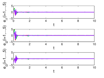
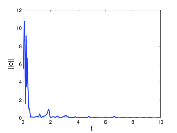
Figure 2: The counterpart synchronization error between the drive layer (1) and the response layer (2) formed by Lü oscillators. Left: $e_{ij}(t)$ varying with time $t$; right: the total synchronization error.

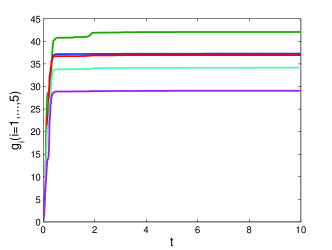
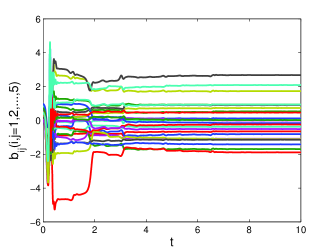
Figure 3: The adaptive feedback gains $g_{i}(t)~{}(i=1,2,...,5)$ (left) and parameters $b_{ij}(t)~{}(i,j=1,2,...,5)$ updating according to (10) (right).

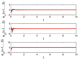
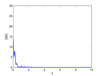
Figure 4: The counterpart synchronization error of a duplex Hindmarsh-Rose neural network. Left: $e_{ij}(t)$ varying with time $t$; right: the total synchronization error.

Example 4.2

Synchronization in neuronal networks is one of the burning problems in neuroscience in recent years, and the Hindmarsh-Rose model [27] has become a popular model for analysis of neuronal activity and has also been extensively investigated. For example, Fang et al. investigated chaotic synchronization of nearest-neighbor diffusive coupling Hindmarsh-Rose neural networks in noisy environments [28], and Zhou et al. discussed the Hindmarsh-Rose model by using impulsive pinning control [29]. In what follows, we will discuss the synchronization between two coupled Hindmarsh-Rose neuronal networks. The Hindmarsh-Rose model can be described by a three-dimensional nonlinear differential equations as follows [27]:

$$\mathbf{\dot{x}}_{i}=\mathbf{f}(t,\mathbf{x}_{i}(t),\mathbf{x}_{i}(t-\tau(t)))$$

$$=\left(\begin{array}[]{lll}x_{i2}(t)-x_{i3}(t)-x_{i1}(t-\tau)^{3}+3x_{i1}(t-\tau)^{2}+I\\ 1-x_{i2}(t)-5x_{i1}(t-\tau)^{2}\\ \mu(4(x_{i1}(t)+\bar{x})-x_{i3}(t))\\ \end{array}\right).$$

Take $I=3,\bar{x}=1.56,\mu=0.006,\sigma_{0}=1,\tau=0.1$. Assumption (H2) is satisfied [24]. The inner coupling matrix $\Gamma=[1~{}1~{}0;0~{}1~{}0;0~{}0~{}1]$. The intra-layer topologies, the noise term and initial states of nodes are taken as the same as those in the previous example. Figure 4 shows counterpart synchronization errors between two unidirectionally connected Hindmarsh-Rose networks. Figure 5 further presents the updated feedback gains $g_{i}(t)~{}(i=1,2,...,5)$ and adaptive parameters $b_{ij}(t)~{}(i,j=1,2,...,5)$. It is clearly seen that the numerical simulations perfectly match the theoretical results.

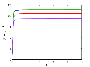
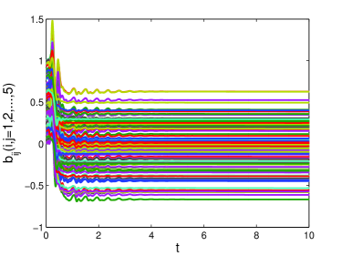
Figure 5: The adaptive feedback gains $g_{i}(t)~{}(i=1,2,...,5)$  (left) and parameters $b_{ij}(t)~{}(i,j=1,2,...,5)$ updating according to (10)  (right).

5 Conclusions

In this paper, counterpart synchronization of duplex networks with delayed nodes and noise perturbation has been investigated. Based on the LaSalle-type invariance principle for stochastic differential equations, a sufficient condition guaranteeing CS with the proposed control scheme has been provided. Numerical examples have also been presented to illustrate the effectiveness of method. The proposed method will find its applicability to a wide range of practical duplex networks.

6 Acknowledgments

This work is supported by the National Natural Science Foundation of China under Grants 61174028, 61203159, 41201418 and 41301442.

7 References

References

• [1] Kurths J, Pikovsky A and Rosenblum M 2003 Synchronization: A Universal Concept in Nonlinear Sciences vol 415 (Physics Today)
• [2] Boccaletti S, Latora V, Moreno Y, Chavez M and Hwang D U 2006 Phys. Rep. 424 175–308
• [3] Osipov G V, Kurths J and Zhou C 2009 Synchronization in Oscillatory Networks (Springer Berlin)
• [4] Watts D J and Strogatz S H 1998 Nature 393 440–442
• [5] Nishikawa T, Motter A E, Lai Y C and Hoppensteadt F C 2003 Phys. Rev. Lett. 91 014101
• [6] Motter A E, Zhou C and Kurths J 2005 Euro Phys. Lett. 69 334–340
• [7] Pecora L M and Carroll T L 1998 Phys. Rev. Lett. 80 2109
• [8] Huang L, Chen Q, Lai Y C and Pecora L M 2009 Phys. Rev. E 80 036204
• [9] Wang X F and Chen G 2002 Internat. J. Bifur. Chaos Appl. Sci. Engrg. 12 187–192
• [10] Wang X F and Chen G 2002 IEEE Trans. Circuits Syst. I. 49 54–62
• [11] D’Agostino G and Scala A 2014 Networks of Networks: The Last Frontier of Complexity (Springer International Publishing Switzerland)
• [12] Xiong F, Liu Y and Zhang Z 2014 J. Stat. Mech. Theory Exp. 2014 P12026
• [13] Liu W, Schmittmann B, Schmittmann and Zia R K P 2014 J. Stat. Mech. Theory Exp. 2014 P05021
• [14] Wu X, Zheng W X and Zhou J 2009 Chaos 19 013109
• [15] Wu X 2008 Phys. A 387 997–1008
• [16] Zhao J, Li Q, Lu J A and Jiang Z P 2010 Chaos 20 023119
• [17] Zhang S, Wu X, Lu J A, Feng H and Lu J 2014 IEEE Trans. Circuits Syst. I. 61 3216–3224
• [18] Zheng S, Wang S, Dong G and Bi Q 2012 Commun. Nonlinear Sci. Numer. Simul. 17 284–291
• [19] Wang G, Cao J and Lu J 2010 Phys. A: Stat. Mech. Appl. 389 1480–1488
• [20] Wang Y, Lai Y C and Zheng Z 2010 Phys. Rev. E 81 036201
• [21] Nagai K H and Kori H 2010 Phys. Rev. E 81 065202
• [22] Wu X, Zhou C, Chen G and Lu J a 2011 Chaos 21 043129
• [23] Wu X, Wang W and Zheng W X 2012 Phys. Rev. E 86 046106
• [24] Sun Y, Li W and Ruan J 2013 Commun. Nonlinear Sci. Numer. Simul. 18 989–998
• [25] Mao X 1999 J. Math. Anal. Appl. 236 350–369
• [26] Li D, Lu J a, Wu X and Chen G 2006 J. Math. Anal. Appl. 323 844–853
• [27] La Rosa M, Rabinovich M, Huerta R, Abarbanel H and Fortuna L 2000 Phys. Rev. A 266 88–93
• [28] Fang X L, Yu H J and Jiang Z L 2009 Chaos Solitons Fractals 39 2426–2441
• [29] Zhou J, Wu Q and Xiang L 2012 Nonlinear Dyn. 69 1393–1403