On the Bifurcation and Stability of Single and Multiple Vortex Rings in Three-Dimensional Bose-Einstein Condensates

Abstract

In the present work, we investigate how single- and multi-vortex-ring states can emerge from a planar dark soliton in three-dimensional (3D) Bose-Einstein condensates (confined in isotropic or anisotropic traps) through bifurcations. We characterize such bifurcations quantitatively using a Galerkin-type approach, and find good qualitative and quantitative agreement with our Bogoliubov-de Gennes (BdG) analysis. We also systematically characterize the BdG spectrum of the dark solitons, using perturbation theory, and obtain a quantitative match with our 3D BdG numerical calculations. We then turn our attention to the emergence of single- and multi-vortex-ring states. We systematically capture these as stationary states of the system and quantify their BdG spectra numerically. We find that although the vortex ring may be unstable when bifurcating, its instabilities weaken and may even eventually disappear, for sufficiently large chemical potentials and suitable trap settings. For instance, we demonstrate the stability of the vortex ring for an isotropic trap in the large chemical potential regime.

I Introduction

Over the last two decades, there has been an intense interest in nonlinear matter waves in the context of atomic Bose-Einstein condensates (BECs) book1 ; book2 ; emergent . In the three-dimensional (3D) setting, arguably, one of the most prototypical excitations that arise are vortex rings (VRs). Such toroidal-shaped vortices, or rings of vorticity, have been predicted theoretically and observed experimentally in numerous studies; see, e.g., the relevant reviews emergent ; komineas_rev ; book_new . In addition to their relevance in superfluids, VRs are of intense interest in other areas, e.g., in fluid mechanics saffman ; Pismen1999 . Superfluid VRs have been observed experimentally in helium donnelly ; Rayfield64 ; Gamota73 , far before their emergence in atomic BECs of dilute alkali gases. In the atomic BEC setting, these states have arisen in a variety of ways. One such example is through the bending of a 3D vortex line (i.e., a line of vorticity) so that it closes on itself VR:CrowInstab . Vortex rings have also been experimentally realized through the decay of planar dark solitons in two-component BECs Anderson01 , by density engineering Shomroni09 (related to earlier theoretical proposals of Refs. Ruostekoski01 ; Ruostekoski05 ), and in the evolution of colliding symmetric defects Ginsberg05 . They have also been detected through their unusual collisional outcomes of structures that may appear as dark solitons in cigar-shaped traps sengstock .

Numerical studies have also theoretically explored potential methods to generate VRs. Some of these examples involve the flow past an obstacle Jackson99 ; Rodrigues09 , Bloch oscillations in an optical trap Scott04 , the collapse of bubbles Berloff04a , the instability of two-dimensional (2D) rarefaction pulses Berloff02 , the flow past a positive ion Berloff00 ; Berloff00a or an electron bubble Berloff01 , the Crow instability of two vortex pairs Berloff01a and the collisions of multiple BECs Carretero08 ; Carretero08a . VR cores have an intrinsic velocity Roberts71 (a feature that can be understood by considering their cross-section resemblance to a vortex dipole which is well-known to travel at a constant speed saffman ; Pismen1999 ). However, this intrinsic velocity can be counterbalanced by the presence of an external trap, which is commonplace in atomic BECs VR-BEC-STRUCTGOOD . This, in turn, creates the possibility for the existence of stationary VRs, and, in fact, even of multi-rings, as discussed earlier, e.g., in Ref. ionut .

The aim of the present work is to revisit the study of VRs, but from a different perspective to the above works, namely we focus of their bifurcation and emergence in the weakly nonlinear limit. In this sense, our study is partially connected to the recent work of Ref. pantof , where a somewhat similar approach was adopted. Nevertheless, their work focused on a setting where the trapping was only in two out of three spatial directions; another fundamental difference with respect to Ref. pantof is their absence of stability information in the relevant setup. On the other hand, our study is also inspired by the pioneering work of Ref. feder , which, in turn, motivated the experimental results of Ref. Anderson01 . In Ref. feder , the spectrum of a dark soliton was examined (although not in its full detail, as we will discuss below) and some of the key instability mechanisms associated with it were elucidated. We are also motivated by the analysis presented in Refs. middelphysd ; middel2 , which used a somewhat similar approach to that used herein to explore bifurcations from a two-dimensional dark soliton to vortex-dipoles and, more generally, multi-vortex structures.

Our fundamental starting point will be the realization that a VR emerges from a suitable combination of two distinct states with a relative phase (of $\pi/2$ between them), namely a planar dark soliton (say, along the $z$-direction) and of a ring dark soliton (RDS) along the $(x,y)$ plane, another state studied extensively in earlier work; see, e.g., Refs. rds2003 ; herring ; kamch . Should the planar dark soliton have a lower energy than the RDS, then the bifurcation happens from the former; if the order of energies is reversed, then the bifurcation occurs from the RDS. If, however, the energies are equal (which, as we will see, happens for anisotropic traps, i.e., when the trapping frequencies along the $z$- and radial $r$- directions satisfy $\omega_{z}=2\omega_{r}$), the VR state already emerges at the linear (noninteracting) limit. The presence of two principal modes in the coherent structure enables us to adapt a Galerkin-type, two-mode methodology, originally developed for double-well potentials; see, e.g., relevant details in Ref. theochar , based on the fundamental earlier work of Ref. smerzi . This two-mode approach allows us to provide a quantitative estimate, which turns out to not only qualitatively but also quantitatively predict the bifurcation/emergence point of the single VR. We use a similar approach to generalize to more complex states such as the double VR (arising due to the combination of a double-soliton/second excited state along the $z$-axis, with a RDS along the $(x,y)$ plane), and we further extend this approach to single and double vortex lines.

Since the planar dark soliton may spawn the VR, in the appropriate regime, we expand upon the work of Ref. feder by capturing all its modes using the Bogoliubov-de Gennes (BdG) analysis near the linear (small-interaction) limit. This limit enables a perturbative treatment of the relevant modes, both in the isotropic and in the anisotropic case, clearly allowing us to identify neutral modes, modes responsible for instabilities and also the bifurcations of novel states such as the VR, and the single and double solitonic vortex. We provide, both, analytical estimates and full-numerical calculations for the relevant eigenvalues, and provide connections with the analytical two mode theory discussed above. Once the relevant bifurcations arise, especially those leading to the single and double VRs of focal interest herein, we turn our attention to their spectra to quantify instability and the potential stabilization mechanisms. This leads us to conclude that these states tend to be weakly unstable in the small-interaction limit, but may —in principle— be stabilized in the large-interaction setting.

It is relevant to mention that this problem remains of particular interest, not only for theoretical but also for recent experimental studies. A notable example is the very recent work of Ref. zwierlein , where the tomographic imaging of a superfluid Fermi gas of ⁶Li atoms enabled the observation of the snaking instability of the planar dark soliton into a VR (and subsequently into a vortex line). Connecting state-of-the-art observations such as these to the understanding of stationary-state stability offered here should furnish a complete picture of the underlying complex dynamics of the system.

Our presentation is structured as follows. Section II contains the different aspects of our analytical results; first, the bifurcation analysis (of single and double VRs) using the Galerkin method; and second, the spectral analysis, for the small-interaction limit, of the dark solitons which we connect to the above bifurcation structure. In Sec. III, we provide detailed numerical computations of the existence and stability of dark solitons, and subsequently VRs and multi-VRs, starting from the small-interaction limit. We provide comparisons between our numerical and analytical predictions. Finally, in Sec. IV, we summarize our findings and present both, our conclusions, as well as some interesting directions for future studies.

II Analytical Considerations

In this work we utilize the 3D Gross-Pitaevskii equation (GPE), expressed in the following dimensionless form emergent :

$$iu_{t}=-\frac{1}{2}\nabla^{2}u+V(r)u+|u|^{2}u.$$ (1)

Here, $u$ is the macroscopic wavefunction of the 3D BEC near zero temperature, while the potential assumes the prototypical parabolic form, namely:

$$V(x,y,z)=\frac{1}{2}\omega_{r}^{2}r^{2}+\frac{1}{2}\omega_{z}^{2}z^{2}.$$ (2)

The parameters $\omega_{r}$ and $\omega_{z}$ represent the trapping strengths along the $(x,y)$ plane and $z$ direction, respectively, with the spherically symmetric (isotropic) case corresponding to $\omega_{r}=\omega_{z}$.

II.1 Vortex Ring Bifurcation Near the Linear Limit

In the linear limit, Eq. (1) reduces to the quantum harmonic oscillator (QHO), with energy spectrum:

$$E_{n,m,k}=\omega_{r}\left(n+m+1\right)+\omega_{z}\left(k+1/2\right),$$ (3)

where $n$, $m$ and $k$ are the non-negative integers indexing the corresponding eigestate. Let us now discuss how to construct a VR starting from the considered linear limit. Intriguingly, utilizing the results of Ref. ionut , this is possible in the following way: in that work it was found that for the anisotropic trap with $\omega_{r}=1$ and $\omega_{z}=2/k$ the energy of a second radial excited state ($m$,$n$,$k^{\prime}$) with $m+n=2$ and $k^{\prime}=0$ (i.e. $E=3+1/k$) coincides with that of the $k$-th excited state along the $z$-axis $(0,0,k)$ (also equal to $1+(2/k)(k+1/2)=3+1/k$). For such anisotropic traps one can construct stationary states with $k$-parallel-VRs

$$u(x,y,z)\propto\frac{|2,0,0\rangle+|0,2,0\rangle}{\sqrt{2}}+i|0,0,k\rangle,$$ (4)

even at the linear limit. The RDS nature of the real part combined with the $k$ oscillations of the imaginary part along the $z$-direction constitutes parallel VRs with alternating vorticity. Remarkably, this is a very natural 3D generalization of the 2D setting considered in Ref. middelphysd . In the above expression of Eq. (4), we have used the notation

$$|n,m,k\rangle = H_{n}(\sqrt{\omega_{r}}x)H_{m}(\sqrt{\omega_{r}}y)H_{k}(\sqrt{\omega_{z}}z)$$ (5)

$$\times \exp[-(\omega_{r}(x^{2}+y^{2})+\omega_{z}^{2}z^{2})/2],$$

corresponding to the eigenmode of energy $E_{n,m,k}$ of the QHO where $H$ represents the Hermite polynomials.

Generalizing the approach of Ref. middelphysd by considering anisotropic trap strengths $\omega_{r}$ and $\omega_{z}$ (including the isotropic one of $\omega_{r}=\omega_{z}$), the energies of the RDS and the $k$-th solitonic state will, respectively be,

$$E_{\rm RDS}=3\omega_{r}+\frac{\omega_{z}}{2},\quad{\rm and}\quad E_{\rm sol}=\omega_{r}+(k+\frac{1}{2})\omega_{z}.$$

Hence, for $k\omega_{z}<2\omega_{r}$, the state of lower energy will be the $k$-th soliton from which the $k$-th VR will bifurcate, while for $k\omega_{z}>2\omega_{r}$, the lower energy will belong to the RDS, with the bifurcation occurring from that state.

II.1.1 Single vortex ring, $\omega_{z}<2\omega_{r}$

Following the bifurcation phenomenology of Ref. middelphysd (see also Ref. middel2 ), we first consider the limit $\omega_{z}<2\omega_{r}$ which encompasses the isotropic trap, and proceed as follows. Take the $k$-th soliton along the $z$-axis, focusing for now on $k=1$, and assign this as mode $u_{1}$ with energy $E_{1}$. Similarly, assign the RDS as mode $u_{2}$ with energy $E_{2}$. If a novel state (in this case, the single VR) bifurcates from these two states when their phase difference is $\pi/2$, then a general two-mode analysis theochar predicts that the number of atoms $N=\int|u|^{2}dxdydz$ at the bifurcation critical point will be given by

$$N_{\rm cr}=\frac{E_{1}-E_{2}}{I_{12}-I_{11}},$$ (6)

where for the above special case of the single VR we have $E_{1}-E_{2}=\omega_{z}-2\omega_{r}$, while $I_{11}=\int|u_{1}|^{4}dxdydz$ and $I_{12}=\int|u_{1}|^{2}|u_{2}|^{2}dxdydz$ are overlap integrals. Specifically, for the VR, the dark soliton state from which the bifurcation arises is $u_{1}=|0,0,1\rangle$, while the RDS is $u_{2}=\frac{|2,0,0\rangle+|0,2,0\rangle}{\sqrt{2}}$.

Furthermore, the general two-mode theory also predicts the chemical potential value at which the bifurcation will occur, namely

$$\mu_{\rm cr}=E_{1}+I_{11}N_{\rm cr},$$ (7)

where $N_{\rm cr}$ is given by Eq. (6).

Interestingly, the above integrals can be computed analytically. In particular, for the case of the single VR with $k=1$, we find that

$$I_{11}=\frac{3\omega_{r}\sqrt{\omega_{z}}}{8\sqrt{2}\pi^{3/2}}=3I_{12}.$$ (8)

As a result, the explicit prediction for the bifurcation of the VR is that:

$$N_{\rm cr}^{\rm(VR,1)} = \frac{4\sqrt{2}\pi^{3/2}(2\omega_{r}-\omega_{z})}{\omega_{r}\sqrt{\omega_{z}}},$$ (9)

$$\mu_{\rm cr}^{\rm(VR,1)} = 4\omega_{r}.$$ (10)

This provides us with an explicit prediction for the bifurcation of the first VR.

II.1.2 Single vortex ring, $\omega_{z}>2\omega_{r}$

For completeness, we now consider the case of $\omega_{z}>2\omega_{r}$, where the VR now bifurcates from the RDS and the subscripts of Eq. (6) must be exchanged 1$\leftrightarrow$2. For this case, $E_{2}-E_{1}=2\omega_{r}-\omega_{z}$ and $I_{22}=\int|u_{2}|^{4}dxdydz=2I_{12}$, which leads to the bifurcation point:

$$N_{\rm cr}^{\rm(VR,2)} = \frac{8\sqrt{2}\pi^{3/2}(\omega_{z}-2\omega_{r})}{\omega_{r}\sqrt{\omega_{z}}}$$ (11)

$$\mu_{\rm cr}^{\rm(VR,2)} = \frac{5}{2}\omega_{z}-\omega_{r}.$$ (12)

The superscripts in Eqs. (9) and (10) versus those of Eqs. (11) and (12) are used to illustrate which state the VR bifurcates from, 1 is for the dark soliton and 2 represents the RDS.

II.1.3 Double vortex rings, $\omega_{z}<\omega_{r}$

Similarly, for the double-vortex-ring (2VR) state $E_{1}-E_{2}=2(\omega_{z}-\omega_{r})$, while the overlap integrals are given by

$$I_{11}=\frac{41\omega_{r}\sqrt{\omega_{z}}}{128\sqrt{2}\pi^{3/2}}=\frac{41}{12}I_{12}.$$ (13)

Hence, the corresponding prediction for the bifurcation point yields

$$N_{\rm cr}^{\rm(2VR,1)} = \frac{256\sqrt{2}\pi^{3/2}(\omega_{r}-\omega_{z})}{29\omega_{r}\sqrt{\omega_{z}}},$$ (14)

$$\mu_{\rm cr}^{\rm(2VR,1)} = \frac{222\omega_{r}-19\omega_{z}}{58}.$$ (15)

These predictions are valid for $\omega_{z}\leq\omega_{r}$. In this case, the 2VR will bifurcate from the two-dark-soliton state of the form $u_{1}=|0,0,2\rangle$, while the higher energy state in the two-mode analysis will again be the RDS.

II.1.4 Double vortex rings, $\omega_{z}>\omega_{r}$

On the other hand, for $\omega_{z}>\omega_{r}$ the prediction needs to be suitably modified. Since the 2VR now bifurcates from the RDS we again exchange the subscripts in Eq. (6). Using $I_{22}=(41\omega_{r}\sqrt{\omega_{z}})/(128\sqrt{2}\pi^{3/2})$ (for $u_{2}=|0,0,2\rangle$) we finally find that:

$$N_{\rm cr}^{\rm(2VR,2)} = \frac{64\sqrt{2}\pi^{3/2}(\omega_{z}-\omega_{r})}{5\omega_{r}\sqrt{\omega_{z}}},$$ (16)

$$\mu_{\rm cr}^{\rm(2VR,2)} = \frac{37\omega_{z}-2\omega_{r}}{10}.$$ (17)

An interesting feature is the following. For $\omega_{z}<2\omega_{r}$, the single VR bifurcates from the one-dark soliton ($k=1$) and for $\omega_{z}<\omega_{r}$ the 2VR bifurcates from the two-dark-soliton state ($k=2$). In the “intermediate” case, $\omega_{r}<\omega_{z}<2\omega_{r}$, the 2VR state bifurcates from the RDS, while the single VR bifurcates from the one-dark soliton. Finally, for $2\omega_{r}<\omega_{z}$, both the single VR and the 2VR states bifurcate from the RDS. Hence, as expected, $\mu_{\rm cr}^{\rm(2VR,2)}>\mu_{\rm cr}^{\rm(VR,2)}$, i.e. first the lower-energy single VR bifurcates, followed by the 2VR state.

We remark in passing that, in line with the special-case results of Ref. ionut , the single VR bifurcates from the linear limit ($N\rightarrow 0$) in the anisotropic case of $\omega_{z}=2\omega_{r}$, as per Eq. (9), while the 2VR bifurcates from the linear limit, precisely for the isotropic case of $\omega_{z}=\omega_{r}$, as per Eq. (14). One can similarly generalize these types of bifurcation considerations for all higher-order rings, providing an explicit set of predictions for their emergence in the vicinity of the linear limit. This bifurcation and stability analysis naturally explains why the decay of dark solitonic states yields the corresponding $k$-VR states, not only in numerical simulations feder , but also in experiments Anderson01 .

II.1.5 Solitonic vortices

While the emphasis here is on VRs, partly to illustrate that the different states obtained in Ref. pantof can be identified with the techniques presented herein, we also provide other special cases, namely the single- and double-solitonic vortex states.

For the case $\omega_{z}<\omega_{r}$, following the same technique as above but with $u_{2}=|1,0,0\rangle$, we obtain:

$$N_{\rm cr}^{\rm(1SV,1)} = \frac{4\sqrt{2}\pi^{3/2}(\omega_{r}-\omega_{z})}{\omega_{r}\sqrt{\omega_{z}}},$$ (18)

$$\mu_{\rm cr}^{\rm(1SV,1)} = \frac{5\omega_{r}}{2},$$ (19)

for the single solitonic vortex (bifurcating from the dark soliton $u_{1}=|0,0,1\rangle$). For the double solitonic vortex, again bifurcating from $u_{1}=|0,0,1\rangle$ but with $u_{2}=(|2,0,0\rangle-|0,2,0\rangle)/\sqrt{2}$, one finds the bifurcation point:

$$N_{\rm cr}^{\rm(2SV,1)} = \frac{4\sqrt{2}\pi^{3/2}(2\omega_{r}-\omega_{z})}{\omega_{r}\sqrt{\omega_{z}}},$$ (20)

$$\mu_{\rm cr}^{\rm(2SV,1)} = 4\omega_{r},$$ (21)

for $\omega_{z}<2\omega_{r}$. The reverse trap anisotropies can similarly be explored.

II.1.6 Comparison to other work

Finally, and before proceeding with the stability analyses of the dark soliton and the resulting VR states that are the principal focus of the present work, let us compare our work to Ref. pantof . Our existence results bear significant resemblance to those of Ref. pantof , although there are also nontrivial differences. For instance, in Ref. pantof the focus was on bifurcations from the dark soliton (called the kink therein) state, whereas we especially focus on bifurcations from various states that yield VR-like solutions (single and double VRs). In Ref. pantof , the $z$-direction is presumed to be homogeneous (i.e., untrapped), while here we consider the presence of a trap. For this reason, multi-VR states (such as those explored above) are not possible in the framework of Ref. pantof . In fact, the 2VR state in that work is one in which both rings are in the same plane, while here we explore multiple non-coplanar rings in a stationary state, rendered possible by the additional trapping along the $z$-direction. On a technical level too, the methodology of the reduction to a quasi-linear equation on the plane with an effective potential used in Ref. pantof , while ingenious, differs substantially from the two-mode approach utilized herein. Finally, and perhaps most importantly, a principal focus that stems from our existence findings is that, we also study the stability of the obtained solutions (see details in the following section). In Ref. pantof , on the other hand, this is deferred to future studies.

II.2 Stability Analysis Near the Linear Limit

We now move to the stability analysis in the vicinity of the linear limit. Using a Taylor expansion of the solution $u=\sqrt{\epsilon}u_{0}+\epsilon^{3/2}u_{1}+\dots$ and $\mu=\mu_{0}+\epsilon\mu_{1}+\dots$ in Eq. (1), where $(\mu_{0},u_{0})$ correspond, respectively, to the eigenvalue and eigenfunction of a state at the linear limit, we find at O$(\epsilon)$ the solvability condition:

$$\mu_{1}=\int|u_{0}|^{4}dxdydz.$$ (22)

This, in turn, allows us to specify $\epsilon=(\mu-\mu_{0})/\mu_{1}$ (to leading order). Then, the spectral stability, as discussed in Ref. feder , amounts to solving the BdG eigenvalue problem $({\cal H}_{0}+\epsilon{\cal H}_{1})U=\omega U$, with

$$U =\left(\begin{array}[]{c}\mathcal{U}\\ \mathcal{V}\\ \end{array}\right),$$ (25)

$${\cal H}_{0} =\left(\begin{array}[]{cc}{\cal L}&0\\ 0&-{\cal L}\\ \end{array}\right),$$ (28)

where ${\cal L}=-(1/2)\nabla^{2}+V(r)-\mu_{0}$, while

$${\cal H}_{1}=\left(\begin{array}[]{cc}2|u_{0}|^{2}-\mu_{1}&u_{0}^{2}\\ -(u_{0}^{2})^{\star}&\mu_{1}-2|u_{0}|^{2}\\ \end{array}\right),$$ (31)

where the star denotes complex conjugate. Here, we denote $\omega$ as the eigenfrequency of a given eigenstate $U$ with eigenvalue $\lambda=i\omega$. The presence of a nonzero imaginary part of $\omega$ or, equivalently, of a nonzero real part of $\lambda$ in our Hamiltonian system denotes the presence of a dynamical instability.

II.2.1 The dark soliton

From the above formulation, it is straightforward to analyze the stability in the case of $\epsilon\rightarrow 0$. There, it is evident that the linearization spectrum consists of the diagonal contributions of ${\cal H}_{0}$ which consist of the spectrum of ${\cal L}$ and of its opposite. Up to now, we have kept our exposition as general as possible, but from here on, we will focus on a specific state in order to showcase the relevant ideas more concretely. As our workhorse, we will use the dark soliton state $u_{0}=|0,0,1\rangle$, in a spirit similar to that of Ref. feder , but with a particular view towards the bifurcation of the VR state (as well as others such as the 2VR and the single and double solitonic vortex). Since ${\cal L}$ consists of the quantum harmonic oscillator, the spectrum for a dark soliton along the $z$-axis, when subtracting $\mu_{0}=\omega_{r}+3\omega_{z}/2$, will be (see Eq. (3))

$$\omega=\omega_{r}\left(n+m\right)+\omega_{z}(k-1).$$ (32)

Recalling that $n$, $m$, and $k$ are arbitrary non-negative integers, we now proceed to explore the relevant states and their multiplicities. The mode with $n=m=k=0$ corresponds to the negative energy book2 ; feder , or negative Krein signature kks , mode. Such a mode, when resonant with another positive energy (or Krein signature) one, will give rise to complex eigenvalue quartets, while collisions of modes of the same energy will be inconsequential towards changing the stability properties of the solution. The dark soliton state (with vanishing density in the $z=0$ plane) has a neutral mode, corresponding to $(n,m,k)=(0,0,1)$, which has a wavefunction identical to the solution itself. This mode corresponds to the phase or gauge (U$(1)$) invariance of Eq. (1). There are three additional Kohn modes corresponding to symmetry which are also left invariant. Specifically, $(n,m,k)=(0,0,2)$ corresponds to dipolar oscillations along the $z$-axis with frequency $\omega=\omega_{z}$, while the modes $(n,m,k)=(1,0,1)$ and $(n,m,k)=(0,1,1)$ pertain to dipolar oscillations along the $(x,y)$-plane with frequency $\omega=\omega_{r}$. To complete our discussion of modes with $n+m+k\leq 2$, we need to account for five more modes. There are two degenerate modes (due to the radial invariance of the trap in the plane) of $(n,m,k)=(1,0,0)$ and $(n,m,k)=(0,1,0)$, with frequency $\omega=\omega_{r}-\omega_{z}$ and three degenerate ones, $(n,m,k)=(2,0,0)$, $(n,m,k)=(0,2,0)$ and $(n,m,k)=(1,1,0)$, all of which have frequency $\omega=2\omega_{r}-\omega_{z}$ in the linear limit.

II.2.2 The dark soliton, $\omega_{r}=\omega_{z}$

The key question that subsequently arises is that of the fate of the eigenvalues described above, as $\epsilon$ becomes finite, i.e., as we depart from the linear limit. To follow these eigenvalues, and given that the different degeneracies also hinge on the specific values of $\omega_{r}$ and $\omega_{z}$, we will use as our benchmark case the isotropic scenario of $\omega_{r}=\omega_{z}=1$, where the choice of unity is made without loss of generality. In this case, the zero eigenvalue has a multiplicity of three. The gauge-invariance mode must remain at zero, and so too must the two modes (1,0,0) and (0,1,0) due to the spherical invariance of the dark soliton solution, but only when the trap is isotropic.

We now move to the consideration of the principal $7$ modes (recall that this is really 7 pairs) at $\omega=\pm 1$. Out of these, the 3 dipolar modes will remain invariant. Then, however, 4 modes are subject to deviations, as soon as we depart from the linear limit. It turns out that the insightful work of Ref. feder has already computed one sub-manifold associated with such a bifurcation. In that work, the authors recognized that the eigenvector associated with the RDS $U_{1}=(\frac{|2,0,0\rangle+|0,2,0\rangle}{\sqrt{2}},0)^{T}$ [see Eq. (25)] and the anomalous mode $U_{2}=(0,|0,0,0\rangle)^{T}$ become resonant, and identified the deviations by using degenerate perturbation theory, i.e., constructing the matrix ${\cal M}$ with

$${\cal M}_{ij}=\langle U_{i}|{\cal H}_{1}|U_{j}\rangle,$$ (33)

and identifying its eigenvalues for $i,j=1,2$ for the above eigenvectors. That calculation, adapted to the present setting, can be rewritten as

$$\omega=1-\frac{\left(3\pm i\sqrt{7}\right)}{12}\left(\mu-\frac{5}{2}\right)$$ (34)

(cf. Eq. (20) in Ref. feder ). It is important to note that the near-linear prediction is that the dark soliton should be immediately unstable due to this resonant interaction, via an oscillatory instability and a quartet of corresponding eigenvalues. This is a general feature that dark soliton (and multi-soliton) states possess near the linear limit due to the degeneracy of their anomalous modes; cf. the work of Ref. coles . However, in that work these instability “bubbles” were shown to terminate at some finite value of $\mu$, hence it is of interest to explore whether a similar feature arises here, a question that we will address below numerically.

On the other hand, in the work of Ref. feder , an additional (and, as we will see, important) sub-manifold of eigenvectors was not considered, namely that of $U_{1}=(\frac{|2,0,0\rangle-|0,2,0\rangle}{\sqrt{2}},0)^{T}$ and of $U_{2}=(|1,1,0\rangle,0)^{T}$. For this subspace, we find that the corresponding deviation of the eigenfrequency from the linear limit —again, obtained via the degenerate perturbation theory of Eq. (33)— yields:

$$\omega=1-\frac{2}{3}\left(\mu-\frac{5}{2}\right).$$ (35)

Given the decreasing trend of both of these eigenvalues, it is natural to expect that at some finite value of $\mu$, they will hit the origin of the spectral plane. As a preamble to our numerical computations of the next section, it is then relevant to consider what the outcome of such a collision will be. Connecting these findings with our bifurcation theory results of the previous subsection, we appreciate that these collisions should be, in fact, what leads to the corresponding bifurcations and destabilizations of the dark soliton along the $z=0$ plane. In particular, the mode $U_{1}=(\frac{|2,0,0\rangle+|0,2,0\rangle}{\sqrt{2}},0)^{T}$ effectively corresponds to the RDS. Its “collision” with the origin and subsequent destabilization of the dark soliton along the $z=0$ plane suggests that beyond this threshold the planar dark soliton and RDS mesh, which, as we have discussed before, produces the single VR state. In the same spirit, we can see that the collision of $U_{1}=(\frac{|2,0,0\rangle-|0,2,0\rangle}{\sqrt{2}},0)^{T}$ with the origin will produce a meshing with the planar dark soliton and lead to the bifurcation of the two solitonic vortex state, discussed in the previous subsection. In fact, assuming the prediction of Eq. (35) to be useful beyond its realm of validity (and until $\omega=0$) yields a critical point for the relevant bifurcation at $\mu=4$, which coincides with the prediction of $\mu^{\rm(2SV,1)}$ of Eq. (21). We will numerically examine the validity of these predictions in the next section.

II.2.3 The dark soliton, $\omega_{r}=2\omega_{z}$

In principle, the approach adopted above (and the associated eigenvalue count and deviations from the linear limit) can be used for any state bifurcating from the linear limit. However, obviously, the more complicated the original state, the more difficult it becomes to account for all the relevant eigenvalues. Since our focus here is on VRs and their emergence, we will also give an additional example of the case of $\omega_{r}=2\omega_{z}=1$ (more generally bearing in mind the case of $\omega_{r}\neq\omega_{z}$), which will be considered in our numerical eigenvalue analysis below. Once again, in this case, 4 modes remain invariant, namely one at $\omega=0$ (phase invariance), and at $\omega=\omega_{z}$ and (double) $\omega=\omega_{r}$ due to the dipolar oscillations. The manifold of the modes $(1,0,0)$ and $(0,1,0)$ with frequency $\omega=\omega_{r}-\omega_{z}$ at the linear limit leads to the prediction (using again degenerate perturbation theory)

$$\omega=\left(\omega_{r}-\omega_{z}\right)-\frac{1}{3}\left[\mu-(\omega_{r}+\frac{3}{2}\omega_{z})\right].$$ (36)

On the other hand, the anomalous mode of indices $(0,0,0)$ is theoretically predicted to move according to

$$\omega=\omega_{z}-\frac{1}{6}\left[\mu-(\omega_{r}+\frac{3}{2}\omega_{z})\right].$$ (37)

Then, the sub-manifold of eigenvectors with $U_{1}=(\frac{|2,0,0\rangle-|0,2,0\rangle}{\sqrt{2}},0)^{T}$ and of $U_{2}=(|1,1,0\rangle,0)^{T}$ produces two coincident eigenfrequencies (actually two pairs) with

$$\omega=\left(2\omega_{r}-\omega_{z}\right)-\frac{2}{3}\left(\mu-(\omega_{r}+\frac{3}{2}\omega_{z})\right).$$ (38)

However, we can see that there are additional eigenvalues, in this case, that acquire comparable values and therefore manifolds of larger sum $n+m+k$ need to be considered (up to now we had restricted considerations to $n+m+k=2$). Among the eigenvalues with $n+m+k=3$, the case of $(0,0,3)$ will have an eigenfrequency of $\omega=1$ in the present setting. The perturbative calculation in this case yields a prediction of

$$\omega=2\omega_{z}-\frac{1}{12}\left[\mu-(\omega_{r}+\frac{3}{2}\omega_{z})\right].$$ (39)

Even more complicated are the degeneracies occurring at $\omega=1.5$. In addition to $U_{1}=(\frac{|2,0,0\rangle-|0,2,0\rangle}{\sqrt{2}},0)^{T}$ and of $U_{2}=(|1,1,0\rangle,0)^{T}$ considered above, there is the double degeneracy of $U_{1}=(\frac{|2,0,0\rangle+|0,2,0\rangle}{\sqrt{2}},0)^{T}$ and $U_{2}=(|0,0,4\rangle,0)^{T}$ and finally that of $U_{1}=(|1,0,2\rangle,0)^{T}$ and $U_{2}=(|0,1,2\rangle,0)^{T}$. The latter, leads to the degenerate eigenfrequencies (again, two pairs) of the form:

$$\omega=\left(\omega_{r}+\omega_{z}\right)-\frac{5}{12}\left[\mu-(\omega_{r}+\frac{3}{2}\omega_{z})\right].$$ (40)

The former eigenvalues (i.e., the RDS and the one with $k=4$) are only resonant when $\omega_{r}=2\omega_{z}$. In this particular case, we can obtain the corresponding eigenfrequencies

$$\omega=1.5-\frac{53\pm 7\sqrt{73}}{192}\left(\mu-\frac{7}{4}\right).$$ (41)

We believe it is clear that while the relevant methodology is entirely general, the logistics of its application vary from case to case and can be fairly complex. For this reason, we now corroborate and complement our analysis with detailed numerical computations in the following section. The above two case studies, of the isotropic regime and of $\omega_{r}=2\omega_{z}$, will operate as our benchmarks. We will also numerically explore other settings such as $\omega_{z}=2\omega_{r}$ as well as, importantly, the spectra of our states of particular focus, namely the bifurcating (single and double) VRs.

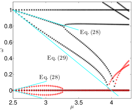
Figure 1: (color online) Spectrum for the dark soliton stationary state for the isotropic case, $\omega_{r}=\omega_{z}$. Depicted are the eigenfrequencies stemming from the BdG analysis, as a function of the chemical potential. Real parts of the eigenfrequencies are denoted by black cross points, while the imaginary parts of the eigenfrequencies are denoted by red plus points. The blue solid lines correspond to theoretical predictions in the small-interaction, linear, limit (cf. text).

III Numerical Results

We identify the stationary solutions by solving the Gross-Pitaevskii equation using a Newton-Krylov scheme kelly . The Bogoliubov linearization spectrum is then obtained by utilizing a spectral basis of noninteracting modes; at least 800 are used for each result herein. From a numerical standpoint, the problem is reduced to two dimensions by utilizing a Fourier-Hankel method ronen (see also Ref. blakie ), which is made possible by the azimuthal symmetry of the trap in the $(x,y)$ plane.

Recall that in Bogoliubov theory every eigenfrequency belongs to a pair, having solutions of opposite sign. From here on, we simplify our discussion by only plotting half of the spectrum, one eigenfrequency from each of these pairs.

III.1 The dark soliton, $\omega_{r}=\omega_{z}$

We begin our discussion by considering dark soliton stationary state for the isotropic case, $\omega_{r}=\omega_{z}=1$. The corresponding results are depicted in Fig. 1; a typical example of the solution itself (both planar cuts, as well as a full 3D density isocontour plot) is shown in Fig. 2. A first observation is that our analytical predictions seem to agree well in the linear limit with the corresponding numerical results. More specifically, we observe that the complex quartet of Eq. (34) indeed destabilizes the planar dark soliton in the linear limit, as was originally observed in Ref. feder . However, as we depart from this limit, the phenomenology reported in Ref. coles appears to arise, namely the resonant interaction of the RDS mode and of the anomalous mode ceases. Thereafter, the anomalous mode maintains a roughly constant frequency, while the RDS rapidly decreases in frequency, eventually colliding with the origin (i.e., with $\omega=0$) for a value of $\mu=4.05$ (very close to the theoretical predictions of $\mu=4$, see Eq. (10)). Indeed, beyond this critical point, this eigenfrequency becomes imaginary (equivalently, the eigenvalue becomes real), giving rise to a symmetry-breaking pitchfork bifurcation. The daughter branch emerging from this bifurcation (per our analysis), is the single VR (of charge either $+1$ or $-1$). This will be further corroborated by the computation of this state below.

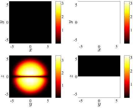
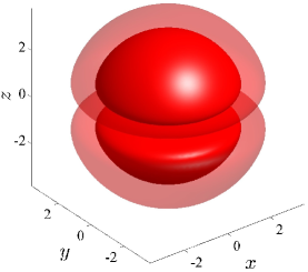
Figure 2: (color online) Dark soliton state for the isotropic case of $\omega_{r}=\omega_{z}=1$ and $\mu=12$. The top four panels show the modulus of the solution (left subpanels) and their respective argument $\theta$ (right subpanels). The top row illustrates the $z=0$ plane, where the density vanishes, and the middle row shows the $x=0$ plane. The bottom panel shows two isocontour density plots for this state (the contours correspond to iso-density surfaces at the maximum density divided by 2.5 and 1.5).

Furthermore, we can observe a good agreement also for the two degenerate eigenfrequencies, stemming from $U_{1}=(\frac{|2,0,0\rangle-|0,2,0\rangle}{\sqrt{2}},0)^{T}$ and $U_{2}=(|1,1,0\rangle,0)^{T}$ (where $U$ is defined in Eq. (25), in accordance with Eq. (35). In this case too, the decrease in frequency eventually leads to a zero-crossing and a destabilization of the dark soliton state in favor, in this case, of a double solitonic vortex (2SV) state. It is important to note that, contrary to the homogeneous (along $z$) case reported in Ref. pantof , here the bifurcation of the 2SV and that of the single VR do not occur at the same value of the chemical potential. A consequence of this is that the dark soliton has already been destabilized by the bifurcation of the 2SV state when the VR bifurcates, and hence the VR in this isotropic case is expected to inherit this weak instability close to that limit. Note that there are three modes that are invariant at $\omega=0$, one of which is due to the gauge invariance, and two have frequency $\omega_{r}-\omega_{z}=0$, reflecting the rotational invariance of the planar dark soliton.

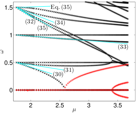
Figure 3: (color online) Spectrum for the dark soliton stationary state for $\omega_{r}=2\omega_{z}=1$. Points have the same meaning as in Fig. 1.

III.2 The dark soliton, $\omega_{r}=2\omega_{z}$

We now turn to the investigation of our second analytically examined case, namely of $\omega_{r}=2\omega_{z}=1$. The comparison between the analytical prediction and the numerical results for the stability spectrum is depicted in Fig. 3. Remarkably, we can see in this case too —despite the considerable complexity of the bifurcation diagram— the high accuracy of our eigenvalue predictions near the linear limit. While in this case there is no quartet from the linear limit, the instability emerges due to the rapid decrease of the modes (accurately predicted by Eq. (36), near the linear limit) pertaining to the manifold of $(1,0,0)$ and $(0,1,0)$. We remark that, in the isotropic case, this pair of modes was equi-energetic with the dark soliton, allowing the construction from the linear limit of the single solitonic vortex. Here, however, it is at $\mu=2.58$ that the relevant instability emerges, giving rise to the solitonic vortex state. Notably, this also agrees with the analytical prediction of $\mu=2.5$, see Eq. (19). The only other instability that can be observed is given by the collision of the RDS, predicted by Eq. (41), with the anomalous mode of Eq. (37). This, once again, leads to a quartet of eigenfrequencies and only for considerably larger values of $\mu$ (not included in the figure) will the VR bifurcate. Additional predictions such as the manifold of $U_{1}=(\frac{|2,0,0\rangle-|0,2,0\rangle}{\sqrt{2}},0)^{T}$ and of $U_{2}=(|1,1,0\rangle,0)^{T}$ through Eq. (38), as well as the higher index ($n+m+k$) of Eqs. (39) and (40) are also reasonably accurately captured.

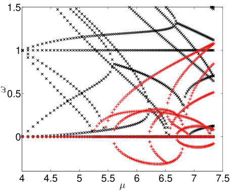
Figure 4: (color online) Spectrum for the dark soliton stationary state for $\omega_{r}=\omega_{z}/2=1$. Otherwise, similar to Fig. 1. Here the ring dark soliton and the planar dark soliton have the same energy, and hence the VR can bifurcate immediately from the linear limit. The principal instabilities of the dark soliton in this case arise due to higher modes (with $n+m=3$), although lower-order modes contribute to oscillatory instabilities associated with complex eigenfrequency quartets.

III.3 The dark soliton, $\omega_{z}=2\omega_{r}$

Finally, we also touch upon the case of $\omega_{z}=2\omega_{r}=2$ —cf. Fig. 4. In this case, the situation is considerably more complex and numerous instabilities appear to arise. Nevertheless, in this case too, our understanding of the linear limit may provide a reasonable set of guidelines for understanding the relevant phenomenology. In this case, we observe four instabilities associated with imaginary eigenfrequencies and three associated with eigenfrequency quartets. Among the latter, the first to arise is the degenerate pair (the cross states) of eigenfrequencies, emerging from the origin with negative energy and colliding with a higher-order (in $n+m+k$) mode at $\mu=5.59$. The second quartet begins at $\mu=6.21$ and involves the RDS (arising from the origin with negative energy) colliding with a higher energy mode. It should be remarked that the presence of the RDS at the linear limit enables (as discussed earlier) the bifurcation of the VR already at the linear limit. This, in turn, implies that the VR may be expected to be robust in this case (however, see the detailed results below). Finally, the third collision involves the degenerate modes $(1,0,0)$ and $(0,1,0)$ which are also now anomalous due to their negative energy and are growing from the linear limit. This pair collides with higher order modes and a quartet develops for $\mu>6.69$. The first two imaginary instabilities arising are, surprisingly, not caused by lower-order modes, but rather from the higher-order ones $(3,0,0)$ and $(0,3,0)$, as well as from $(1,2,0)$ and $(2,1,0)$. Both of these sets of eigenfrequency pairs decrease, as we depart from the linear limit, leading to an imaginary eigenfrequency instabilities for $\mu>5.24$ and $\mu>5.44$, respectively. Hence, we see that in this case too, we can form a qualitative picture of the stability landscape merely by knowing and suitably appreciating the linear eigenfrequency/eigenmode picture.

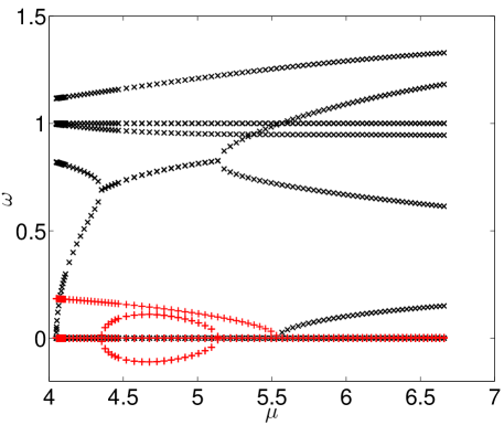
Figure 5: (color online) Single VR for $\omega_{r}=\omega_{z}$. Similar to that of Fig. 1, the present figure shows the BdG spectrum (this spectrum coincides with that of the dark soliton when the VR bifurcates from the it at $\mu=4.05$; cf. Fig. 1). Notice that despite oscillatory and imaginary eigenfrequency-related instabilities (discussed in the text) for small values of $\mu$, the VR is stabilized in the large chemical potential limit.

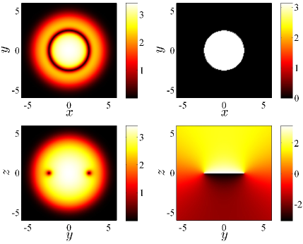
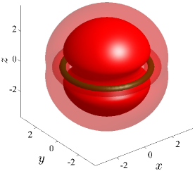
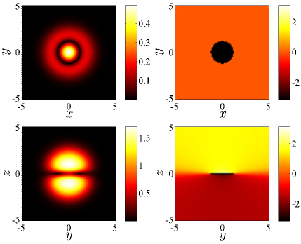
Figure 6: (color online) Single VR state for $\omega_{r}=\omega_{z}=1$. Similar layout as in Fig. 2. The cross sections of the top two rows and the density isocontour of the middle panel show a prototypical example of the bifurcating branch (for $\mu>4.05$) of the single VR in the large chemical potential limit (here at $\mu=12$), where the relevant state has been stabilized against small-amplitude perturbations. The darker (green) isocontour corresponds to an iso-density at the maximum density divided by 8 plotted inside the bulk of the cloud. The bottom two rows correspond to a VR solution right after its bifurcation at $\mu=4.05$, clearly illustrating its ring dark soliton character in the $(x,y)$ plane and its “emerging vorticity” in the phase which is reminiscent of a vortex dipole (despite the resemblance with a dark soliton in the density).

III.4 The single vortex ring, $\omega_{r}=\omega_{z}$

We now turn our attention to the case of the VR, first considering the isotropic trap; see Fig. 5 for the BdG spectrum and Fig. 6 for an illustration of the relevant state far from (top two rows) and near to (bottom two rows) its bifurcation point. As expected, the eigenfrequency pertaining to the RDS $U_{1}=(\frac{|2,0,0\rangle+|0,2,0\rangle}{\sqrt{2}},0)^{T}$, grows along the real axis. Recall that, for the dark-soliton stationary state, the RDS was the mode that became unstable and gave rise to the VR. However, for larger values of the chemical potential (i.e., for $\mu\in[4.35,5.14]$), and in a way reminiscent to what happens for the dark soliton in the vicinity of the linear limit, the RDS collides with the anomalous, negative energy mode $U_{2}=(0,|0,0,0\rangle)^{T}$, giving rise to an oscillatory instability (and an associated eigenfrequency quartet). This instability disappears for larger values of $\mu>5.14$.

Importantly, since the VR bifurcated from the dark soliton state (both with $\omega_{r}=\omega_{z}$) then at the point of bifurcation their spectra should be identical, cf. Figs. 1 and 5 at $\mu=4.05$. Recall, though, that at the bifurcation point another instability was already present in the spectrum of the dark soliton due to the prior bifurcation of the 2SV. Consequently, the VR is endowed with this instability from birth. However, upon increase of the chemical potential, we observe that the eigenfrequency associated with this inherited instability (corresponding to a doubly degenerate subspace associated with $U_{1}=(\frac{|2,0,0\rangle-|0,2,0\rangle}{\sqrt{2}},0)^{T}$ and of $U_{2}=(|1,1,0\rangle,0)^{T}$, i.e., the “cross states”) decreases and eventually leads to a complete stabilization of the VR for $\mu>5.54$. It is due to this stabilization that such VR patterns can be observed robustly in the large chemical potential (Thomas-Fermi) limit. In the latter limit, the VR acquires particle-like characteristics; see, e.g., Ref. horng for the dynamics of a single VR inside a trap and Ref. caplan for the interactions between multiple VRs. The combination of these features and the connection of the spectral features of the VR with the above particle-like characteristics will be explored separately in a future publication.

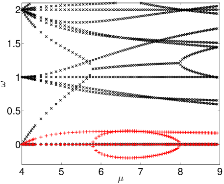
Figure 7: (color online) Spectrum for the single VR when $\omega_{r}=\omega_{z}/2=1$, similar to Fig. 5. Here, the VR emerges from the linear limit.

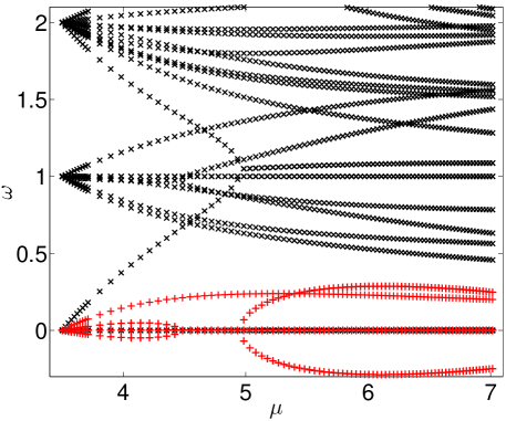
Figure 8: (color online) Spectrum for the double vortex ring (2VR) for the isotropic case $\omega_{r}=\omega_{z}=1$. Points have the same meaning as previous figures.

III.5 The single vortex ring, $\omega_{z}=2\omega_{r}$

We now briefly examine the VR for the special case where it bifurcates from the linear limit, namely when $\omega_{z}=2\omega_{r}$ (and hence the energies of the dark soliton and the RDS become degenerate, enabling the construction of a VR already at the linear limit, in accordance with Eq. (4)). The corresponding BdG spectrum is depicted in Fig. 7. Interestingly, here, we observe that the VR is, in fact, unstable immediately (i.e., as soon as we depart from the linear limit). This instability is manifested through a degenerate imaginary pair of eigenfrequencies, again associated with the cross states $U_{1}=(\frac{|2,0,0\rangle-|0,2,0\rangle}{\sqrt{2}},0)^{T}$ and of $U_{2}=(|1,1,0\rangle,0)^{T}$. In this limit, the latter states also bifurcate from the linear limit and apparently have lower energy than the VR. We note, however, that as we proceed to larger values of the chemical potential, the instability appears to (weakly) decrease and, hence, VRs may again be long-lived in the Thomas-Fermi limit of large $\mu$. Additionally, it is worthwhile to note that once again the collision of $U_{1}=(\frac{|2,0,0\rangle+|0,2,0\rangle}{\sqrt{2}},0)^{T}$ with the anomalous mode $U_{2}=(0,|0,0,0\rangle)^{T}$ leads to a resonance and an oscillatory instability for the interval $5.78\leq\mu\leq 8.00$.

We also remark that, for this stationary state as well, the relevant eigenvalue count can be performed. Consider the eigenvalues of the operator ${\cal L}-\mu_{0}$ (with $\mu_{0}=4\omega_{r}$) to be $\omega_{r}(n+m+2k)-2\omega_{r}$. We find that there are (a) 4 modes at the spectral plane origin (3 climb from the origin with increasing $\mu$, as discussed above, and one remains at the origin due to gauge invariance), there are (b) 8 modes at $\omega=\omega_{r}$, two of which are anomalous, while there are (c) 10 modes at $\omega=2\omega_{r}$, one of which is anomalous and gives rise to the oscillatory instability discussed above. Hence, given the technical complications of considering the relevant perturbative analysis (and also the qualitative understanding afforded to us by means of the above analysis), we will not pursue this further here.

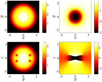
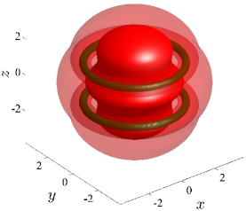
Figure 9: (color online) Double VR (2VR) state for the isotropic case $\omega_{r}=\omega_{z}=1$ and $\mu=12$. Similar layout as in Figs. 2 and 6. This state bifurcates from the linear limit at $\mu=7\omega_{r}/2$.

III.6 The double vortex ring, $\omega_{z}=\omega_{r}$

Finally, we also examine the double-vortex ring (2VR) state, bifurcating from the linear limit of $\mu_{0}=7\omega_{r}/2$ in the isotropic case of $\omega_{r}=\omega_{z}$, see Figs. 8 and 9. Here the situation is even more complicated, with 6 degenerate eigenfrequencies at $\omega=0$, 13 modes (3 anomalous ones) at $\omega=\omega_{r}$, and so on. Hence, we will again restrict our considerations to some qualitative remarks. We note that the state will be immediately unstable in this isotropic limit, due to an imaginary eigenfrequency pair (the cross states), bifurcating from $0$ as soon as the 2VR state emerges. Moreover, the resonance of the degenerate anomalous pair at $\omega=\omega_{r}$ with the corresponding positive (same) energy modes leads to a scenario again reminiscent of Ref. coles in that an oscillatory instability emerges from the linear limit, although it is terminated at $\mu=4.47$. An additional collision of a mode bifurcating from the origin with the anomalous mode $U_{2}=(0,|0,0,0\rangle)^{T}$ leads to an additional eigenfrequency quartet for $\mu>4.96$. A key observation here is that these instabilities (both the imaginary one and the oscillatory one for $\mu>4.96$) were found to persist throughout the interval of parameters considered herein. However, for large values of $\mu$, we observe a weak tendency for both of these instabilities towards decreasing growth rates. The latter feature appears to be qualitatively consonant with the observations of Ref. ionut , suggesting that, for intermediate parameters, 2VR states were less robust than for large values of the corresponding nonlinearity-controlling parameter. Once again, the theme of the Thomas-Fermi limit will be the subject of separate work, focusing on the dynamics and interactions of VRs as particle entities.

IV Conclusions and Future Challenges

In conclusion, we have systematically examined the full eigenvalue spectrum by linearization around a dark soliton in a 3D setting, building on considerable earlier work, most notably that of Ref. feder . Extending that work, we have shown how to predict not only the formation and bifurcation of the (single) vortex ring state, but also of other states, such as the double-vortex-ring, the single- and the double-solitonic vortices, among others. We have explained how the emergence of these states can be predicted on the basis of a Galerkin-type, two-mode, approach. This is analogous to how a vortex pair, and more complex states involving multiple vortices, were predicted to arise in 2D (see, e.g., Refs. middelphysd ; middel2 ), a step that subsequently led to their experimental realization hallpra . We have explored the conditions necessary for the vortex ring to emerge through a bifurcation from the planar dark soliton state, and explained when it can arise from the linear limit (when the energy of the ring dark soliton and that of the dark soliton coincide). Conversely, the vortex ring may arise through a bifurcation from the ring dark soliton, when the latter possesses lower energy than the planar dark soliton state. We have also highlighted similarities and differences from important related work such as the contribution of Ref. pantof .

In addition to giving a qualitative characterization of the relevant spectra and bifurcations, in the vicinity of the linear limit, we also employed perturbation theory (often in its more complex degenerate form) in order to quantitatively characterize the eigenvalues responsible for the relevant instabilities and the emergence of new branches.

Upon obtaining a systematic understanding of when the vortex rings arise, we turned our attention to their spectral stability properties, by numerically solving the Bogoliubov-de Gennes equations. We thus found that at the isotropic limit, the single vortex ring may be unstable “at birth”, but can be stabilized at higher chemical potentials. In the anisotropic case, where the vortex ring state emerges from the linear limit, it is also immediately unstable but this instability can be relatively weak in different parametric regimes, such as that of large chemical potential. Similar features were found for the double vortex ring, in qualitative agreement with earlier dynamical observations ionut .

We believe that this study paves the way for a deeper understanding of such vortex ring states, offering an unprecedented view of their spectral features. In this light, there are numerous aspects worthy of further exploration. A more technical example involves the attempt to systematically characterize the spectrum of multiple vortex rings in the special cases where they emerge in the linear limit, i.e., at $\omega_{z}=2\omega_{r}/k$ for the $k$-th vortex ring state. A more intriguing aspect for our considerations is to explore the opposite limit more systematically, namely the Thomas-Fermi realm, where the single and multiple vortex rings possess particle characteristics. While in this area there is some work already done, it is rather incomplete. For instance, in Ref. horng , a theoretical approximation of the vortex ring internal mode spectrum was obtained at this “particle limit”, but it was never tested against the full Bogoliubov-de Gennes spectrum or the three-dimensional GPE. On the other hand, in Ref. caplan , a particle picture is derived and favorably compared to the GPE results, but this is only done in the absence of a trap. Obtaining a conclusive spectral picture for single and multi-vortex rings in the presence of a trap would certainly be of paramount importance for our understanding of the particle-like character of these complex states and of their interactions within trapped BECs. Finally, once these aspects are addressed, one can think of not only examining the role of thermal and/or quantum fluctuations on these rings, but also importantly of generalizing them in multi-component systems, where elaborate spinorial states exist in the form of skyrmions ruost and monopoles simula , among many others. Such studies are currently in progress and will be reported in future publications.

- (1) C.J. Pethick and H. Smith, Bose-Einstein Condensation in Dilute Gases (Cambridge University Press, Cambridge, 2008).
- (2) L.P. Pitaevskii and S. Stringari, Bose-Einstein Condensation (Oxford University Press, Oxford, 2003).
- (3) P.G. Kevrekidis, D.J. Frantzeskakis, and R. Carretero-González (eds.), Emergent Nonlinear Phenomena in Bose-Einstein Condensates. Theory and Experiment (Springer-Verlag, Berlin, 2008).
- (4) S. Komineas, Vortex rings and solitary waves in trapped Bose-Einstein condensates, Eur. Phys. J.- Spec. Topics 147 133 (2007).
- (5) P.G. Kevrekidis, D.J. Frantzeskakis, and R. Carretero-González, The defocusing nonlinear Schrödinger equation: from dark solitons, to vortices and vortex rings (SIAM, Philadelphia, 2015).
- (6) P.G. Saffman, Vortex Dynamics (Cambridge University Press, Cambridge, 1992).
- (7) L.M. Pismen, Vortices in Nonlinear Fields (Clarendon, Oxford, 1999).
- (8) R.J. Donnelly, Quantized Vortices in Helium II (Cambridge University Press, Cambridge, 1991).
- (9) G.W. Rayfield and F. Reif, Quantized vortex rings in superfluid helium, Phys. Rev. 136, A1194–A1208 (1964).
- (10) G. Gamota, Creation of quantized vortex rings in superfluid helium, Phys. Rev. Lett. 31, 517–520 (1973).
- (11) T.P. Simula, Crow instability in trapped Bose-Einstein condensates, Phys. Rev. A 84, 021603(R) (2011).
- (12) B.P. Anderson, P.C. Haljan, C.A. Regal, D.L. Feder, L.A. Collins, C.W. Clark, and E.A. Cornell, Watching dark solitons decay into vortex rings in a Bose-Einstein condensate, Phys. Rev. Lett. 86, 2926–2929 (2001).
- (13) I. Shomroni, E. Lahoud, S. Levy, and J. Steinhauer, Evidence for an oscillating soliton/vortex ring by density engineering of a Bose-Einstein condensate, Nat. Phys. 5, 193–197 (2009).
- (14) J. Ruostekoski and J.R. Anglin, Creating vortex rings and three-dimensional skyrmions in Bose-Einstein condensates, Phys. Rev. Lett. 86, 3934–3937 (2001).
- (15) J. Ruostekoski and Z. Dutton, Engineering vortex rings and systems for controlled studies of vortex interactions in Bose-Einstein condensates, Phys. Rev. A 72, 063626 (2005).
- (16) N. S. Ginsberg, J. Brand, and L.V. Hau, Observation of hybrid soliton vortex-ring structures in Bose-Einstein condensates, Phys. Rev. Lett. 94, 040403 (2005).
- (17) C. Becker, K. Sengstock, P. Schmelcher, P.G. Kevrekidis, and R. Carretero-González, Inelastic collisions of solitary waves in anisotropic Bose-Einstein condensates: sling-shot events and expanding collision bubbles, New J. Phys. 15, 113028 (2013).
- (18) J.F. McCann B. Jackson, and C. S. Adams, Vortex rings and mutual drag in trapped Bose-Einstein condensates, Phys. Rev. A 60, 4882–4885 (1999).
- (19) A.S. Rodrigues, P.G. Kevrekidis, R. Carretero-González, D.J. Frantzeskakis, P. Schmelcher, T.J. Alexander, and Yu. S. Kivshar, Spinor Bose-Einstein condensate past an obstacle, Phys. Rev. A 79, 043603 (2009).
- (20) R. G. Scott, A.M. Martin, S. Bujkiewicz, T.M. Fromhold, N. Malossi, O. Morsch, M. Cristiani, and E. Arimondo, Transport and disruption of Bose-Einstein condensates in optical lattices, Phys. Rev. A 69, 033605 (2004).
- (21) N.G. Berloff and C.F. Barenghi, Vortex nucleation by collapsing bubbles in Bose-Einstein condensates, Phys. Rev. Lett. 93, 090401 (2004).
- (22) N.G. Berloff, Evolution of rarefaction pulses into vortex rings, Phys. Rev. B 65, 174518 (2002).
- (23) N.G. Berloff, Vortex nucleation by a moving ion in a Bose condensate, Phys. Lett. A 277, 240–244 (2000).
- (24) N.G. Berloff and P.H. Roberts, Motions in a Bose condensate: VII. Boundary-layer separation, J. Phys. A: Math. Gen. 33, 4025 (2000).
- (25) N.G. Berloff and P.H. Roberts, Motion in a Bose condensate: VIII. The electron bubble, J. Phys. A: Math. Gen. 34, 81 (2001).
- (26) N.G. Berloff and P.H. Roberts, Motion in a Bose condensate: IX. Crow instability of antiparallel vortex pairs, J. Phys. A 34, 10057 (2001).
- (27) R. Carretero-González, B.P. Anderson, P.G. Kevrekidis, D.J. Frantzeskakis, and N. Whitaker, Dynamics of vortex formation in merging Bose-Einstein condensate fragments, Phys. Rev. A 77, 033625 (2008).
- (28) R. Carretero-González, N. Whitaker, P.G. Kevrekidis and D.J. Frantzeskakis, Vortex structures formed by the interference of sliced condensates, Phys. Rev. A 77, 023605 (2008).
- (29) P. H. Roberts and J. Grant, Motions in a Bose condensate I. The structure of the large circular vortex, J. Phys. A: Gen. Phys. 4, 55–72 (1971).
- (30) C.H. Hsueh, S.C. Gou, T.L. Horng, and Y.M. Kao, Vortex-ring solutions of the Gross-Pitaevskii equation for an axisymmetrically trapped Bose-Einstein condensate, J. Phys. B 40, 4561–4571 (2007).
- (31) L.-C. Crasovan, V.M. Pérez-García, I. Danaila, D. Mihalache, and L. Torner, Three-dimensional parallel vortex rings in Bose-Einstein condensates, Phys. Rev. A 70, 033605 (2004).
- (32) A. Munoz-Mateo and J. Brand, Chladni Solitons and the Onset of the Snaking Instability for Dark Solitons in Confined Superfluids, Phys. Rev. Lett. 113, 255302 (2014).
- (33) D.L. Feder, M.S. Pindzola, L.A. Collins, B.I. Schneider, and C.W. Clark, Dark soliton states of Bose-Einstein condensates in anisotropic traps, Phys. Rev. A 62, 053606 (2000).
- (34) S. Middelkamp, P.G. Kevrekidis, D.J. Frantzeskakis, R. Carretero-González, and P. Schmelcher, Emergence and stability of vortex clusters in Bose-Einstein condensates: A bifurcation approach near the linear limit, Physica D 240, 1449 (2011).
- (35) S. Middelkamp, P.G. Kevrekidis, D.J. Frantzeskakis, R. Carretero-González, and P. Schmelcher, Bifurcations, stability, and dynamics of multiple matter-wave vortex states, Phys. Rev. A 82, 013646 (2010).
- (36) G. Theocharis, D. J. Frantzeskakis, P. G. Kevrekidis, B. A. Malomed, and Yu.S. Kivshar, Ring Dark Solitons and Vortex Necklaces in Bose-Einstein Condensates, Phys. Rev. Lett. 90, 120403 (2003).
- (37) G. Herring, L. D. Carr, R. Carretero-González, P. G. Kevrekidis, and D. J. Frantzeskakis, Radially symmetric nonlinear states of harmonically trapped Bose-Einstein condensates, Phys. Rev. A 77, 023625 (2008)
- (38) A.M. Kamchatnov and S.V. Korneev, Dynamics of ring dark solitons in Bose-Einstein condensates and nonlinear optics, Phys. Lett. A 374, 4625 (2010).
- (39) G. Theocharis, P.G. Kevrekidis, D.J. Frantzeskakis, and P. Schmelcher, Symmetry breaking in symmetric and asymmetric double-well potentials, Phys. Rev. E 74, 056608 (2006).
- (40) S. Raghavan, A. Smerzi, S. Fantoni, and S.R. Shenoy, Coherent oscillations between two weakly coupled Bose-Einstein condensates: Josephson effects, oscillations, and macroscopic quantum self-trapping, Phys. Rev. A 59, 620 (1999).
- (41) M.J.H. Ku, B. Mukherjee, T. Yefsah and M.W. Zwierlein, From planar solitons to vortex rings and lines: cascade of solitonic excitations in a superfluid Fermi gas, arXiv:1507.01047.
- (42) T. Kapitula, P.G. Kevrekidis, and B. Sandstede, Counting eigenvalues via the Krein signature in infinite-dimensional Hamiltonian systems, Physica D 195, 263 (2004); see also ibid 201 (2005) 199.
- (43) M.P. Coles, D.E. Pelinovsky, and P.G. Kevrekidis, Excited states in the large density limit: a variational approach, Nonlinearity 23, 1753 (2010).
- (44) C. T. Kelly, Solving Nonlinear Equations with Newton’s Method, (SIAM, Philadelphia, 2003).
- (45) S. Ronen, D. C. E. Bortolotti, and J. L. Bohn, Bogoliubov modes of a dipolar condensate in a cylindrical trap, Phys. Rev. A 74, 013623 (2006).
- (46) P. B. Blakie, D. Baillie, and R. N. Bisset, Roton spectroscopy in a harmonically trapped dipolar Bose-Einstein condensate, Phys. Rev. A 86, 021604(R).
- (47) T.-L. Horng, S.-C. Gou, and T.-C. Lin, Bending wave instability of a vortex ring in a trapped Bose-Einstein condensate, Phys. Rev. A 74, 041603 (2006).
- (48) R.M. Caplan, J.D. Talley, R. Carretero-González, and P.G. Kevrekidis, Scattering and leapfrogging of vortex rings in a superfluid, Phys. Fluids 26, 097101 (2014).
- (49) S. Middelkamp, P.J. Torres, P.G. Kevrekidis, D.J. Frantzeskakis, R. Carretero-González, P. Schmelcher, D.V. Freilich, and D.S. Hall, Guiding-center dynamics of vortex dipoles in Bose-Einstein condensates, Phys. Rev. A 84, 011605(R) (2011).
- (50) C.M. Savage and J. Ruostekoski Energetically Stable Particlelike Skyrmions in a Trapped Bose-Einstein Condensate, Phys. Rev. Lett. 91, 010403 (2003).
- (51) V. Pietilä and M. Möttönen Non-Abelian Magnetic Monopole in a Bose-Einstein Condensate, Phys. Rev. Lett. 102, 080403 (2009); V. Pietilä and M. Möttönen, Creation of Dirac Monopoles in Spinor Bose-Einstein Condensates, Phys. Rev. Lett. 103, 030401 (2009); M.W. Ray, E. Ruokokoski, S. Kandel, M.Möttönen, and D.S. Hall, Observation of Dirac Monopoles in a Synthetic Magnetic Field, Nature 505, 657 (2014); M.W. Ray, E. Ruokokoski, K. Tiurev, M.Möttönen, and D.S. Hall, Observation of Isolated Monopoles in a Quantum Field, Science 348, 544 (2015).