The statistical analysis of acoustic phonetic data:
exploring differences between spoken Romance languages.

Abstract

The historical and geographical spread from older to more modern languages has long been studied by examining textual changes and in terms of changes in phonetic transcriptions. However, it is more difficult to analyze language change from an acoustic point of view, although this is usually the dominant mode of transmission. We propose a novel analysis approach for acoustic phonetic data, where the aim will be to statistically model the acoustic properties of spoken words. We explore phonetic variation and change using a time-frequency representation, namely the log-spectrograms of speech recordings. We identify time and frequency covariance functions as a feature of the language; in contrast, mean spectrograms depend mostly on the particular word that has been uttered. We build models for the mean and covariances (taking into account the restrictions placed on the statistical analysis of such objects) and use these to define a phonetic transformation that models how an individual speaker would sound in a different language, allowing the exploration of phonetic differences between languages. Finally, we map back these transformations to the domain of sound recordings, allowing us to listen to the output of the statistical analysis. The proposed approach is demonstrated using recordings of the words corresponding to the numbers from ``one'' to ``ten'' as pronounced by speakers from five different Romance languages.

1 Introduction

Historical and comparative linguistics is the branch of linguistics which studies languages' evolution and relationships. The idea that languages develop historically by a process roughly similar to biological evolution is now generally accepted; see, e.g., Cavalli-Sforza, (1997) and Nakhleh et al., (2005). Pagel, (2009) claims that genes and languages have similar evolutionary behaviour and offers an extensive catalogue of analogies between biological and linguistic evolution. This immediately gives rise to the notion of familial relationships between languages.

However, interest in language kinships is not by any means restricted to linguistics. For example, the understanding of this evolutionary process is helpful for anthropologists and geneticists, while distances between languages are proxies for cultural differences and communication difficulties and can be used as such in sociology and economic models (Ginsburgh and Weber,, 2011). Moreover, the nature of the relationship between languages, and especially the way they are spoken, is a topic of widespread interest for its cultural relevance. We all have our own experience with learning and using different languages (and different varieties within each language) and the effort to find quantitative properties of speech can shed some light on the subject.

The first step in exploring the language ecosystem is to choose how to analyse and measure the differences between languages. A language is a complex entity and its evolution can be considered from many different points of view. The processes of change from one language to another have long been studied by considering textual and phonetic representation of the words (see, e.g., Morpurgo Davies,, 1998, and references therein). This focus on written forms reflects a general normative approach towards languages: for cultural and historical reasons, the way we think about them is focused on the written expression of the words and their ``proper'' pronunciations. However, this is more a social artifact than a reality of the population, as there is great variation within each language depending on socio-economic and physiological attributes, geography and other factors.

The focus of this work is on a more recent development in quantitative linguistics: the study of acoustic phonetic variation, i.e. change in the sounds associated with the pronunciations of words. On the one hand, these provide a complementary way to consider the difference between two languages which can be juxtaposed with the differences measured using textual and phonetic representation. On the other hand, it can be claimed that the acoustic expression of the word is a more natural object of interest, textual and phonetic transcriptions being only the representation used by linguists of the normative (or more careful) pronunciations of words. However, the use of speech recordings from actual speakers is not yet well established in historical linguistics, due to the complexity of speech as a data object, the theoretical challenges on how to deal with the variability within and between languages and the difficulties (or impossibility) of obtaining sound recordings of ancient pronunciations. A notable exception is the use of speech recordings in the field of language variation and change, a branch of sociolinguistics concerned with small scale variation within communities (for example, between younger and older members or particular social groups). Some of the techniques we describe here might also be useful tools to address these kinds of sociolinguistics questions.

Indeed, the analysis of acoustic data highlights one of the fundamental challenges in comparative linguistics, namely that the definition of language is an abstraction that simplifies the reality of speech variability and neglects the somehow continuous geographical spread of spoken varieties, albeit with some clear edges. For example, Grimes and Agard, (1959) describe as a ``useful fiction'' the definition of homogeneous speech communities, i.e. groups of speakers whose linguistic pattern are alike. Given that for most of human history, most speakers of languages were illiterate, spoken characteristics are also likely to be of profound importance in the historical development of languages. The complexity of the data object (speech) and the large amount of variation call for careful consideration from the statistical community and we hope this work will help to arouse attention to this relevant subject.

In the remainder of this paper, we operationalise the term ``language'' to mean a set of recordings of various words in a language or dialect, as spoken on various occasions by a group of speakers, without implying that the vocabulary is complete nor even necessary large. However, the proposed methodology can be applied in a straightforward way to larger and more comprehensive corpora.

We use the expression ``acoustic phonetic data'' to refer to sound recordings of the same word (or other linguistic unit) when pronounced by a group of speakers. In particular, we are interested in the case where multiple speakers from each language are included in the data set, since this allows one to better explore statistically the phonetic characteristics of the language. This is very different from having only repetitions of a word pronounced by a single speaker and it calls for the development of a novel approach.

The aim of our work is to provide a framework where:

1. speech recordings can be analysed to identify features of a language,

2. the variability of speech within the language can be considered,

3. the acoustic differences between languages can be explored on the basis of speech recordings, taking into account intra-language variability.

Among other things, this will allow us to develop a model (in Section 6) to explore how the sound produced by a speaker would be modified when moved towards the phonetic structure of a different language. More specifically we will take into account the variability of pronunciation within each language. This means we explore the variability of the speakers of the language so that we can then understand where a specific speaker is positioned in a space of acoustic variation with respect to the population. This allows us to postulate a path that maps the sound produced by this speaker to that of a hypothetical speaker with the corresponding position in a different language. The idea here is to approximate the same kind of information we can extract when a speaker pronounces words in two different languages in which they are proficient even if we have only monolingual speakers. The observation (audio recordings) of many speakers from each group is essential to understand the intra-language variability and thus the relevance of the inter-language acoustic change. This model has an immediate application in speech synthesis, with the possibility of mapping a recording from one language to another, while preserving the speaker's voice characteristics. This approach could be also extended to modify synthesized speech in such a way that it sounds like the voice of a specific speaker (for example a known actress or a public person). This would be of interest for many commercial applications, from computer gaming to advertising and it is only one example of the methods that can be developed in the framework we provide. More generally, the framework given here addresses the problem of how to separate speaker-specific voice characteristics from language-specific pronunciation details.

The paper is structured as follows. Section 2 describes the acoustic phonetic data that are used to demonstrate our methods. We choose to represent the speech recordings in a time-frequency domain using a local Fourier transform resulting in surface observations, known in signal processing as spectrograms. Therefore, a short introduction to the functional data analysis approach to surface data is given in Section 3. The details of these time-frequency representations, as well as the preprocessing steps needed to remove noise artifacts and time misalignment between the speech recordings are described in Section 4. Section 5 illustrates how to estimate some crucial functional parameters of the population of log-spectrograms and claims that the covariance structures are common across all the words in each language. Section 6 is devoted to the definition and exploration of cross-linguistic phonetic differences and shows how the pronunciation of a word can be morphed into another language while preserving the speaker/voice identity. The final section gives a discussion of the advantages of the proposed method and of how it is possible to extend it to even more complex situations, where the phonetic features depend continuously on historical or geographical variables.

2 The Romance digits data set

The methods in this paper will be illustrated with an application to a data set of audio recordings of digits in Romance languages. This data set was compiled in the Phonetics Laboratory of the University of Oxford in 2012-2013. It consists of natural speech recordings of five languages: French, Italian, Portuguese, American Spanish and Castilian Spanish, the two varieties of Spanish being considered different languages for the purpose of the analysis. The speakers utter the numbers from one to ten in their native language. The data set is inherently unbalanced; we have seven French speakers, five Italian speakers, five American Spanish speakers, five Iberian Spanish speakers and three Portuguese speakers, resulting in a sample of $219$ recordings. The sources of the recordings were either collected from freely available language training websites or standardized recordings made by university students. As this data set consists of recordings made under non-laboratory settings, large variabilities may be expected within each group. This provides a real-world setting for our analysis, and allows us to build models which characterise realistic variation in speech recording, somewhat of a prerequisite for using this model in practice, as field work recordings are often not recorded under laboratory conditions. The data set is also heterogeneous in terms of sampling rate, duration and format. As such, before any phonetic or statistical analysis took place, all data were converted to $16$-bit PCM (pulse code modulation) *.wav files at a sampling rate of $16$ kHz. We indicate each sound recording as $x^{L}_{ik}(t)$, where $L$ is the language, $i=1,\ldots,10$ the pronounced word and $k=1,\ldots,n_{L}$ the speaker, $n_{L}$ being the number of speakers available for language $L$, and $t$ time. This data set has been collected within the scope of Ancient Sounds, a research project with the aim of regenerating audible spoken forms of the (now extinct) earlier versions of Indo-European words, using contemporary audio recordings from multiple languages. More information about this project can be found on the website http://www.phon.ox.ac.uk/ancient_sounds.

Although the cross-linguistic comparison of spoken digits is interesting in its own right, this subset of words can also be considered as representative of a language's vocabulary from a phonetic point of view, meaning that the words used for the numbers in the Romance languages were not chosen to possess any specific phonetic structure. Consequently, we use the word ``language'' as a shorthand for these particular small samples of digit recordings. However, we view this analysis as a proof of concept, and will not focus on the problem of the representativeness of the sample of speakers or words. In view of a broad possible application of the approach which will be outlined, more structured choices of representative words could be taken or specific dialect choices made, but the approach would remain the same.

3 The analysis of surface data

Different representations are available in phonetics to deal with speech recordings (see, e.g. Cooke at al.,, 1993). Many of them share the idea of representing the sound with the distribution of intensities over frequency $\omega$ and time $t$. We choose in particular the power spectral density of the Local Fourier Transform (i.e. the narrow-band Fourier spectrogram), as detailed in Section 4. This widely-used representation is a two-dimensional surface that describes the sound intensity for each time sample in each frequency band. Since we can represent each spoken word as a two dimensional smooth surface, it is natural to employ a functional data analysis approach. Good results have already been obtained applying functional data analysis techniques to acoustic analysis, although in the different context of single language studies, for example in Koenig et al., (2008) and Hadjipantelis et al., (2012). Functional data analysis is appropriate in this context because it addresses problems where data are observations from continuous underlying processes, such as functions, curves or surfaces. A general introduction to the analysis of functional data can be found in Ramsay and Silverman, (2005) and in Ferraty and Vieu, (2006). The central idea is that taking into account the smooth structure of the process helps in dealing with the high dimensionality of the data objects.

In contrast, in most previous quantitative work on pronunciation variation, such as sociolinguistics or experimental phonetics, only one or a few acoustic parameters (one-dimensional time series) are examined, e.g. pitch or individual resonant frequencies. Variations in vowel qualities, for example, are typically represented by just two data points: the lowest two resonant frequencies (the first and second formants) measured at the mid-point of the vowel. Such a two-dimensional representation lends itself well to simple visualization of a large number of observations, in the form of a scatterplot. But although the validity of two-frequency representations of vowels or single-variable representations of pitch or loudness is motivated by decades of prior research, it clearly suffers from two limitations. First, almost all of the available time-frequency-amplitude information in the speech signal is simply discarded as if it were irrelevant. Second, we do not always know in advance which acoustic parameters are most relevant to a particular investigation; therefore, a more holistic approach to analysis of speech signals may be helpful. The methods presented in this paper, which take the entire spectrogram of each audio recording as data objects, enable us to examine and to manipulate a variety of properties of speech that are not easily reduced to a single low-dimensional data point. By considering higher-order statistical properties of the shape of spectrograms, it becomes possible to characterise such notions as the typical pronunciation of a word, what each speaker sounds like (in general, irrespective of what words they are saying), how their pronunciation differs from that of other speakers, and what it is that makes two languages sound different, above and beyond the differences in the words they use and the speakers involved.

More formally, we consider here data objects that are two dimensional surfaces on a bounded domain, as it is the case of spectrograms. Let $X$ be a random surface so that $X\in L^{2}([0,\Omega]\times[0,T])$ and $E[||X^{2}||^{2}]<+\infty$. A mean surface can then be defined as $\mu(\omega,t)=E[X(\omega,t)]$ and the four dimensional covariance function as $c(\omega,\omega^{\prime},t,t^{\prime})=\mathrm{cov}[X(\omega,t),X(\omega^{\prime},t^{\prime})]$.

In practice these surfaces are observed over a finite number of grid points and they are affected by noise; indeed they can be thought of as a noisy image. As noted by Ramsay and Silverman, (2005), ``the term functional in reference to observed data refers to the intrinsic structure of the data rather than to their explicit form''. Thus a smoothing step is needed to recover the regular surfaces that reflect the properties of the underlying process. These surfaces are represented by means of a linear combination of basis functions which span the separable Hilbert space $L^{2}([0,\Omega]\times[0,T])$. In particular, we choose the widely popular method of smoothing splines to estimate a smooth surface $\widetilde{X}(\omega,t)$ from the noisy observation on a regular grid $\mathfrak{X}(\omega_{i},t_{j}),\ i=1,\ldots,n_{\omega},\ j=1,\ldots,n_{t}$.

When analysing a sample of surfaces, we are implicitly assuming that the comparison of their values at the same coordinates $(\omega,t)$ is meaningful. However, this is often not the case when data are measurements of a continuous process such as human speech. For example, different speakers (or even the same speaker in different replicates) can speak faster or slower without this changing the meaningful acoustic information in the recordings. The resulting sound objects are obviously not comparable though, unless this problem is addressed first. This situation is so common in functional data analysis that much work has been devoted to its solution and these techniques are referred to as functional registration (or warping or alignment, see Marron et al., (2014) and references therein for details). In the case of a two dimensional surface, the misalignment can in principle affect both coordinates; this is the case for example in image processing. A two dimensional warping function $h(\omega,t)$ is then needed to align each surface and this is a more complex problem than one-dimensional registration. However, even though we are considering data that are surfaces, the way they are produced, which will be detailed in Section 4, makes it sensible to adjust only for the misalignment on the temporal axis, this being due to different speaking rates, which are not relevant for our goals. On the contrary, we want to preserve the differences on the frequency axis which contains information about the phonetic characteristics of the speakers.

Thus, we apply a mono-dimensional warping to our surface data. If we aim to align a sample of surfaces $\widetilde{X}_{1},\ldots,\widetilde{X}_{N}$, we look for a set of time-warping functions $h_{1}(t),\ldots,h_{N}(t)$ so that the aligned surface will be defined as $X_{1}=\widetilde{X}_{1}(\omega,h_{1}(t)),\ldots,X_{N}=\widetilde{X}_{N}(\omega,h_{N}(t))$. In the next section we will describe how to achieve this in practice for acoustic phonetic data.

Given the smooth and aligned surfaces $X_{1},\ldots,X_{N}$, it is possible to estimate the functional parameters of the underlying process, for example

$$\widehat{\mu}(\omega,t)=\frac{1}{N}\sum_{i=1}^{N}X_{i},\ \ \ \widehat{c}(\omega,\omega^{\prime},t,t^{\prime})=\frac{1}{N-1}\sum_{i=1}^{N}(X_{i}(\omega,t)-\widehat{\mu}(\omega,t))(X_{i}(\omega^{\prime},t^{\prime})-\widehat{\mu}(\omega^{\prime},t^{\prime})).$$

However, the high-dimensionality of the problem makes the estimate for the covariance structure inaccurate or even computationally unfeasible. In Section 5 we introduce some modelling assumptions to make the estimation problem tractable.

4 From speech records to smooth spectrogram surfaces

As mentioned in the previous section, we choose to represent the sound signal via the power spectral density of the local Fourier transform. This means we first apply a local Fourier transform to obtain a two dimensional spectrogram which is function of time (the time instant where we centre the window for the local Fourier transform) and frequency. For the Romance digit data, we use a Gaussian window function $w$ with a window length of ten milliseconds (a reasonable length for the signal to be considered as stationary), defined as $\psi(\tau)=\exp(-\frac{1}{2}(\frac{\tau}{0.005})^{2})$. Since the original acoustic data was sampled at $16$ kHz, this results in a window size of 160 samples per frame and the maximal effective frequency detected is $8$ kHz, the Nyquist frequency of our sampling procedure.

We can compute the local Fourier transform at angular frequency $\omega$ and time $t$ as

$$X^{L}_{ik}(\omega,t)=\int_{-\infty}^{+\infty}x^{L}_{ik}(\tau)\psi(\tau-t)e^{-j\omega\tau}\mathrm{d}\tau.$$

The power spectral density, or spectrogram, defined as the magnitude of the Fourier transform and the log-spectrogram (in decibel), is therefore

$$\mathfrak{S}^{L}_{ik}(\omega,t)=10\log_{10}(|X^{L}_{ik}(\omega,t)|^{2}).$$

Fig. 1 shows an example of a raw speech signal (top panel) and the corresponding log-spectrogram (bottom left panel), for the sound produced by a French speaker pronouncing the word un [œ̃],

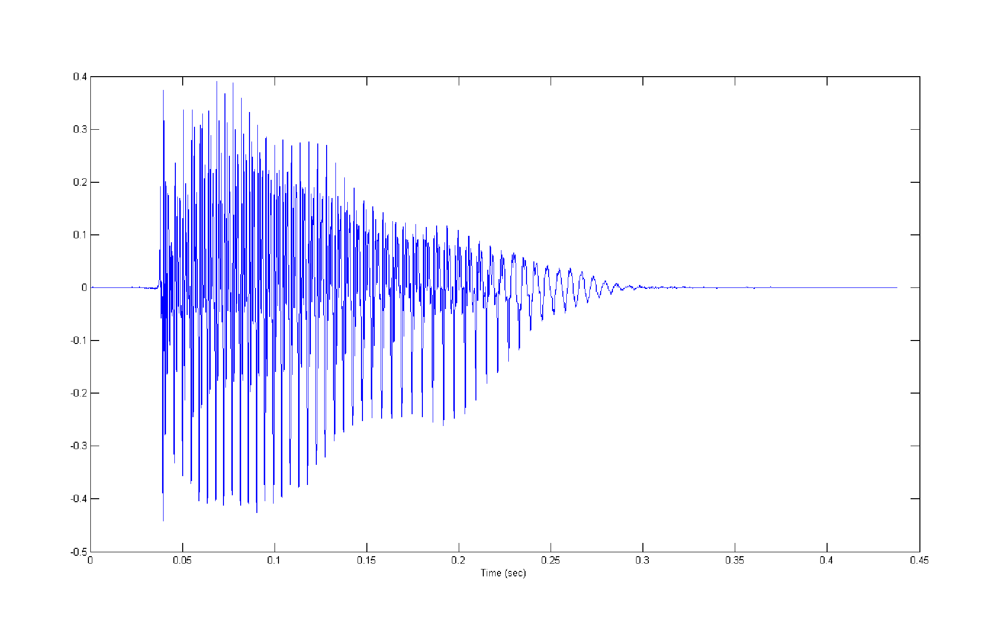
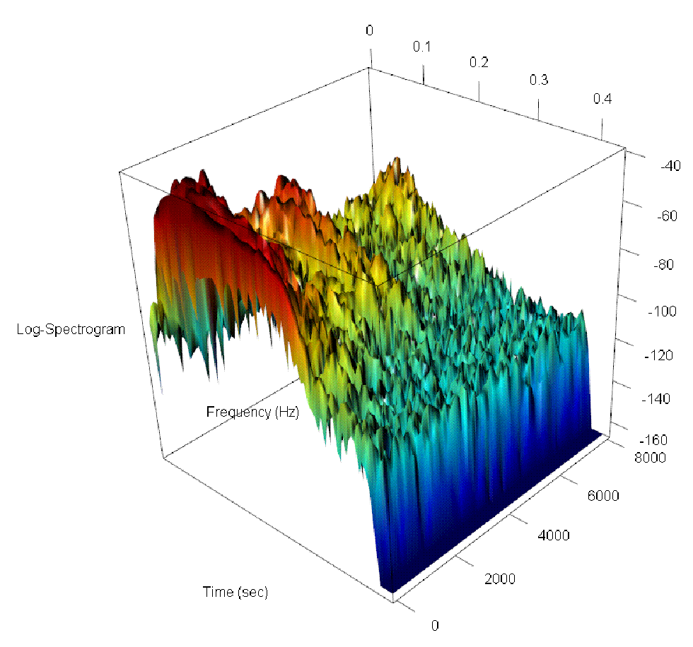
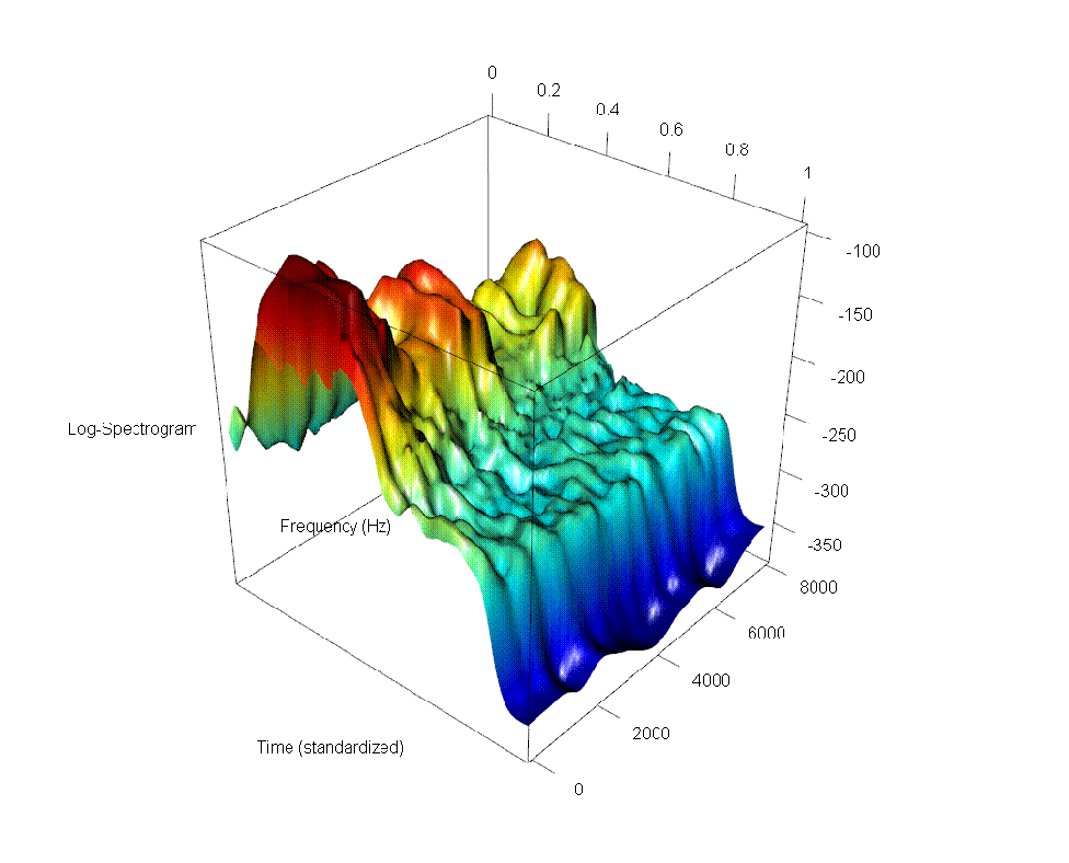
Figure 1: Raw record (top), raw log-spectrogram (bottom left) and smoothed and aligned log-spectrogram (bottom right) for a French speaker pronouncing the word ``un'' (``one'').

To deal with these objects in a functional way, we need to address the problems of smoothing and registration described in the previous section. Indeed, when data comes from real world recordings, as opposed to laboratory conditions, the raw log-spectrograms suffer from noise. For this reason we apply a penalized least square filtering for grid data using discretized smoothing splines. In particular, we use the automated robust algorithm for two-dimensional gridded data described in Garcia, (2010), based on the discrete cosine transform, which allows for a fast computation in high dimensions when the grid is equally spaced. The smoothed log-spectrograms can be transformed back into sounds (via Inverse Fourier Transform) to check that the smoothing removed the noise without loss of any relevant linguistics information.

The second preprocessing step consists of registration in time. This is necessary because speakers can speak faster or slower and this is particularly true when data are collected from different sources where the context is different. However, differences in the speech rate are normally not relevant from a linguistic point of view and thus alignment along the time axis is needed because of this time misalignment in the acoustic signals. First, we standardized the time scale so that each signal goes from $0$ to $1$. Then, we adapt to the case of surface data the procedure proposed in Tang and Müller, (2008) to remove time misalignment from functional observations. Given a sample of functional data $f_{1},\ldots,f_{n}\in L^{2}([0,1])$, this procedure looks for a set of strictly monotone time warping functions $h_{1},\ldots,h_{n}$ so that $h_{i}(0)=0$, $h_{i}(1)=1$, $i=1,\ldots,n$. In practice, these warping functions are modelled via spline functions and estimated by minimizing the pairwise difference between the observed curve while penalizing their departure from the identity warping $h(t)=t$. Hence, a pairwise warping function is first obtained as

$$h_{ij}(t)=\arg\min_{h}\int_{0}^{1}(f_{i}(h(t))-f_{j}(t))^{2}+\lambda\int_{0}^{1}(h(t)-t)^{2},$$

where the minimum is computed over all the spline functions on a chosen grid. Now let $h_{k}$, $k=1,\ldots,n$, be the warping function from a specific time to the standardized time scale. Then, if $s=h_{j}^{-1}(t)$, $h_{i}(s)=h_{i}(h_{j}^{-1}(t))=h_{ij}(t)$. Under the assumption of the warping function to have the identity on average and thus $E[h_{ij}|h_{j}]=h_{j}^{-1}$, the estimator proposed by Tang and Müller, (2008) is

$$h_{j}^{-1}(t)=\frac{1}{n}\sum_{j=1}^{n}h_{ij}(t).$$

To apply this idea to acoustic phonetic data, we need first to define the groups of log-spectrograms we want to align together. As the mean log-spectrogram is different from word to word, we decide to align the log-spectrograms corresponding to the same word. Then, we have to extend the procedure to two dimensional objects such as surfaces. As mentioned in the previous section, it is safe to assume that there is no phase distortion in the frequency direction, given the relatively narrow window used in the local Fourier transform. In contrast, time misalignment can be a serious issue due to differences in speech rate across speakers. Therefore we modify the procedure in Tang and Müller, (2008) so that we look for pairwise time warping functions but minimize the discrepancy between surfaces. For each word $i=1$ in a group of log-spectrograms we want to align, for every pair of languages $L$ and $L^{\prime}$ and for every pair of speakers $k$ and $m$, we define the discrepancy between the log-spectrogram $\widetilde{\mathfrak{S}}^{L}_{ik}$ and $\widetilde{\mathfrak{S}}^{L^{\prime}}_{im}$ as

$$D_{\lambda}(\widetilde{\mathfrak{S}}^{L}_{ik},\widetilde{\mathfrak{S}}^{L^{\prime}}_{im},g^{LL^{\prime}}_{km})=\int_{f=0}^{+\infty}\int_{t=0}^{1}(\widetilde{\mathfrak{S}}^{L}_{ik}(\omega,g^{LL\prime}_{km}(t))-\widetilde{\mathfrak{S}}^{L^{\prime}}_{im}(\omega,t))^{2}+\lambda(g^{LL^{\prime}}_{km}(t)-t)^{2}dtd\omega,$$ (1)

where $\lambda$ is an empirically evaluated non-negative regularization constant and $g^{LL^{\prime}}_{km}(\cdot)$ is the pairwise warping function mapping the time evolution of $\widetilde{\mathfrak{S}}^{L}_{ik}(\omega,t)$ to that of $\widetilde{\mathfrak{S}}^{L^{\prime}}_{im}(\omega,t)$. We obtain the pairwise warping function $\widehat{g}^{LL^{\prime}}_{km}(\cdot)$ by minimizing the discrepancy $D_{\lambda}(\widetilde{\mathfrak{S}}^{L}_{ik},\widetilde{\mathfrak{S}}^{L^{\prime}}_{im},g^{LL^{\prime}}_{km})$ under the constraint that $g^{LL\prime}_{km}$ is piecewise-linear, monotonic and so that $g^{LL^{\prime}}_{km}(0)=0$ and $g^{LL^{\prime}}_{km}(1)=1$. Finally, the inverse of the global warping function for each pronounced word can be estimated as the average of the pairwise warping functions:

$$h^{-1}_{ik}=\frac{1}{\sum_{L^{\prime}=1}^{5}n_{L}}\sum_{L^{\prime}=1}^{5}\sum_{m=1}^{n_{L}}\widehat{g}^{LL^{\prime}}_{km},$$

and the smoothed and aligned log-spectrogram for the language $L$, word $i$ and speaker $k$ is therefore $S_{ik}^{L}(\omega,t)=\widetilde{\mathfrak{S}}^{L}_{ik}(\omega,h_{ik}(t))$. In practice, warping functions are represented with a spline basis defined over a regular grid of $100$ points on $[0,1]$ and we look for the spline coefficients that minimize the discrepancies. The quantities in (1) are approximated by their discretized equivalent on a two-dimensional grid with $100$ equispaced grid points on the time dimension and $81$ equispaced grid points in the frequency dimension. In general, the number of grid points in the time axis needs to be chosen based on the length of the uttered sounds but we have seen that $100$ points provide an accurate reconstruction of the log-spectrograms in the Romance digit dataset.

After this second preprocessing step, we are presented with $219$ smoothed and aligned log-spectrograms. For example, the smoothed and time-aligned log-spectrogram from the sound produced by a French speaker pronouncing the word un can be found in the bottom right panel of Fig. 1.

Other choices are of course possible in the preprocessing of the speech data. In particular, the time registration based on the minimization of the Fisher-Rao metric (Srivastava et al.,, 2011) can be a computationally more efficient alternative when computing time is of concern. By way of example, we also replicate the analysis of the Romance digit data when the smoothing is performed with the thin-plate regression splines implemented in the R package mgcv (Wood,, 2003) and the time registration is obtained by minimising the Fisher-Rao metric (R package fdasrvf, Tucker,, 2014). The results of this alternative analysis are available as supplementary material and are qualitatively similar to the one reported below, giving credence to the idea that the results are not simply systematic mis-registration by one technique versus another.

5 Estimation of means and covariance operators

The process that generates the sounds (and thus their representation as log-spectrograms) is governed by unknown parameters that depend on the language, the word being pronounced and the speaker. However, we need to make some assumptions to identify and estimate these parameters. We consider the mean log-spectrogram as depending on the particular word in each language being pronounced. Indeed, the mean spectrogram is in general different for the different words, as would be expected. Let $i=1,\ldots,10$ be the pronounced words and $k=1,\ldots,n_{L}$ the speakers for the language $L$. The smoothed and aligned log-spectrograms $S_{ik}^{L}(\omega,t)$ allow the estimation of the mean log-spectrogram $\overline{S}_{i}^{L}(\omega,t)=(1/n_{L})\sum_{k=1}^{n_{L}}S_{ik}^{L}(\omega,t)$ for each word $i$ of the language $L$.

Recent studies (Aston et al.,, 2010; Pigoli et al.,, 2014) show that significant linguistic features can be found in the covariance structure between the intensities at different frequencies. This can be considered as a summary of what a language ``sounds like'', without incorporating the differences at the word level. Thus, we first assume in our analysis that the covariance structure of the log-spectrograms is common for all the words in the language and we estimate it using the residual surface obtained by removing the word mean effect. In Section 5.1 we develop a procedure to verify this assumption in the Romance digit data set.

Starting from the smoothed and aligned log-spectrograms $S_{ik}^{L}(\omega,t)$ of the records of the number $i=1,\ldots,10$ for the speakers $k=1,\ldots,n_{i}$, we thus focus on the residual log-spectrograms $R_{ik}^{L}(\omega,t)=S_{ik}^{L}(\omega,t)-(1/n_{i})\sum_{k=1}^{n_{i}}S_{ik}^{L}(\omega,t)$, which measure how each token differs from the word mean. In the following, we disregard in the notation the different speakers and words and for the residual log-spectrogram indicate by $R_{j}^{L}(\omega,t),j=1,\ldots,n_{L}$ the set of observations for the language $L$ including all speakers and words.

However, using standard covariance estimation techniques to find the full four-dimensional covariance structure is computationally expensive or not statistically feasible (because of the small sample size), thus we need some modelling assumptions. There are many ways to incorporate assumptions which allow such estimation, a common one being some form of sparsity. Rather than the usual definition of sparsity that many elements are zero, we prefer to work on the principle that the covariance can be factorised.

We assume that the covariance structure $c^{L}(\omega_{1},\omega_{2},t_{1},t_{2})=cov(S^{L}(\omega_{1},t_{1}),S^{L}(\omega_{2},t_{2}))$ is separable in time and frequency, i.e. $c^{L}(\omega_{1},\omega_{2},t_{1},t_{2})=c^{L}_{\omega}(\omega_{1},\omega_{2})c^{L}_{t}(t_{1},t_{2})$. While we do not necessarily believe this assumption to be true in general, a structure is needed to obtain reliable estimates for the covariance operators, and it is a reasonable assumption that is frequently (implicitly) used in signal processing, particularly when constructing higher dimensional bases from lower dimensional ones.

Possible estimates for $c^{L}_{\omega}(\omega_{1},\omega_{2})$ and $c^{L}_{t}(t_{1},t_{2})$ are

$$\widehat{c}^{L}_{r}=\frac{\widetilde{c}^{L}_{r}}{\sqrt{\mathrm{trace}(\widetilde{c}^{L}_{r})}},\hskip 2.84544ptr=\omega,t,$$ (2)

where $\mathrm{trace}$ indicates the trace of the covariance function, defined as $\mathrm{trace}(c)=\int c(s,s)\mathrm{d}s$, while $\widetilde{c}^{L}_{r}$, $r=\omega,t$ are the sample marginal covariance functions

$$\widetilde{c}^{L}_{\omega}(\omega_{1},\omega_{2})=\frac{1}{n_{L}-1}\sum_{j=1}^{n_{L}}\int_{0}^{1}(R^{L}_{j}(\omega_{1},t)-\overline{R}^{L}_{n_{L}}(\omega_{1},t))(R^{L}_{j}(\omega_{2},t)-\overline{R}^{L}_{n_{L}}(\omega_{2},t))\mathrm{d}t,$$

and

$$\widetilde{c}^{L}_{t}(t_{1},t_{2})=\frac{1}{n_{L}-1}\sum_{j=1}^{n_{L}}\int_{0}^{8\mathrm{kHz}}(R^{L}_{j}(\omega,t_{1})-\overline{R}^{L}_{n_{L}}(\omega,t_{1}))(R^{L}_{j}(\omega,t_{2})-\overline{R}^{L}_{n_{L}}(\omega,t_{2}))\mathrm{d}\omega,$$

$\overline{R}^{L}_{n_{L}}$ being the sample mean of the residual log-spectrogram for the language $L$. We introduce also the associated covariance operators as

$$\widehat{C}^{L}_{r}g(x)=\int_{0}^{M}\widehat{c}^{L}_{r}(x,x^{\prime})g(x^{\prime})\mathrm{d}x^{\prime}\hskip 11.38109ptg\in L^{2}(\mathbb{R}),\hskip 2.84544pt(r,M)\in\{(\omega,8\mathrm{kHz}),(t,1)\}.$$

To see why we choose (2) to estimate the two separable covariance functions, let $\widetilde{c}^{L}_{\omega}$ and $\widetilde{c}^{L}_{t}$ be the true marginal covariance functions, i.e.

$$\widetilde{c}^{L}_{\omega}(\omega_{1},\omega_{2})=\int_{0}^{1}c^{L}(\omega_{1},\omega_{2},t,t)\mathrm{d}t,\ \ \ \widetilde{c}^{L}_{t}(t_{1},t_{2})=\int_{0}^{8\mathrm{kHz}}c^{L}(\omega,\omega,t_{1},t_{2})\mathrm{d}\omega.$$

Then, if the full covariance function is indeed separable, their product can be rewritten as

$$\widetilde{c}^{L}_{\omega}(\omega_{1},\omega_{2})\widetilde{c}^{L}_{t}(t_{1},t_{2})=\int_{0}^{1}c^{L}_{\omega}(\omega_{1},\omega_{2})c^{L}_{t}(t,t)\mathrm{d}t\int_{0}^{8\mathrm{kHz}}c^{L}_{\omega}(\omega,\omega)c^{L}_{t}(t_{1},t_{2})\mathrm{d}\omega=$$

$$=c^{L}_{\omega}(\omega_{1},\omega_{2})\mathrm{trace}(c^{L}_{t})c^{L}_{t}(t_{1},t_{2})\mathrm{trace}(c^{L}_{\omega}).$$

Moreover, $\mathrm{trace}(\widetilde{c}^{L}_{\omega})=\mathrm{trace}(c^{L}_{\omega}\mathrm{trace}(c^{L}_{t}))=\mathrm{trace}(c^{L}_{\omega})\mathrm{trace}(c^{L}_{t})$ and the same is true for $\widetilde{c}^{L}_{t}$. Hence,

$$\frac{\widetilde{c}^{L}_{\omega}(\omega_{1},\omega_{2})}{\sqrt{\mathrm{trace}(\widetilde{c}^{L}_{\omega})}}\frac{\widetilde{c}^{L}_{t}(t_{1},t_{2})}{\sqrt{\mathrm{trace}(\widetilde{c}^{L}_{t})}}=c^{L}_{\omega}(\omega_{1},\omega_{2})c_{t}^{L}(t_{1},t_{2})=c^{L}(\omega_{1},\omega_{2},t_{1},t_{2})$$

and this suggests $\widehat{c}^{L}_{r}$ as estimator for $c^{L}_{r}$, $r=\omega,t$.

Figures 2 and 3 show the estimated marginal covariance functions for the five Romance languages. As can be seen, the frequency covariance functions present differences that appear to be language-specific (with peaks and plateau in different positions), while the time covariances have similar structure, the dependence decreasing when time lag increases and most of the covariability concentrated close to the diagonal.

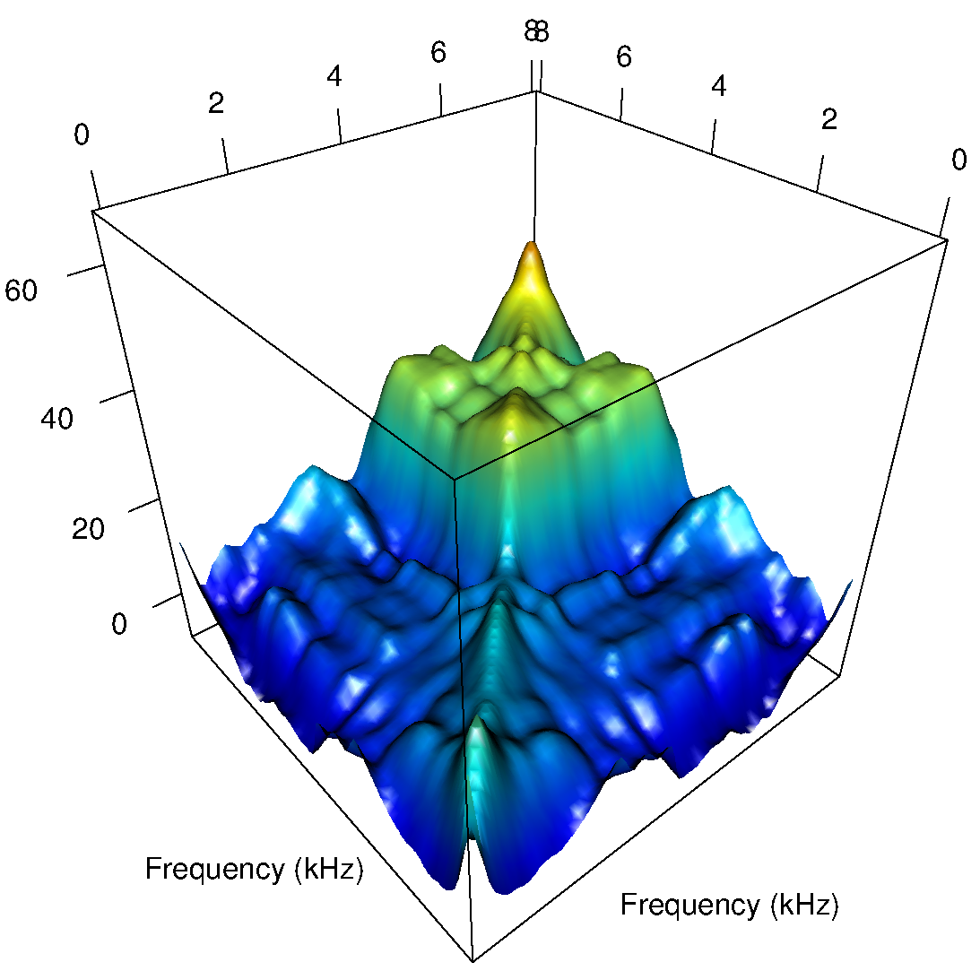
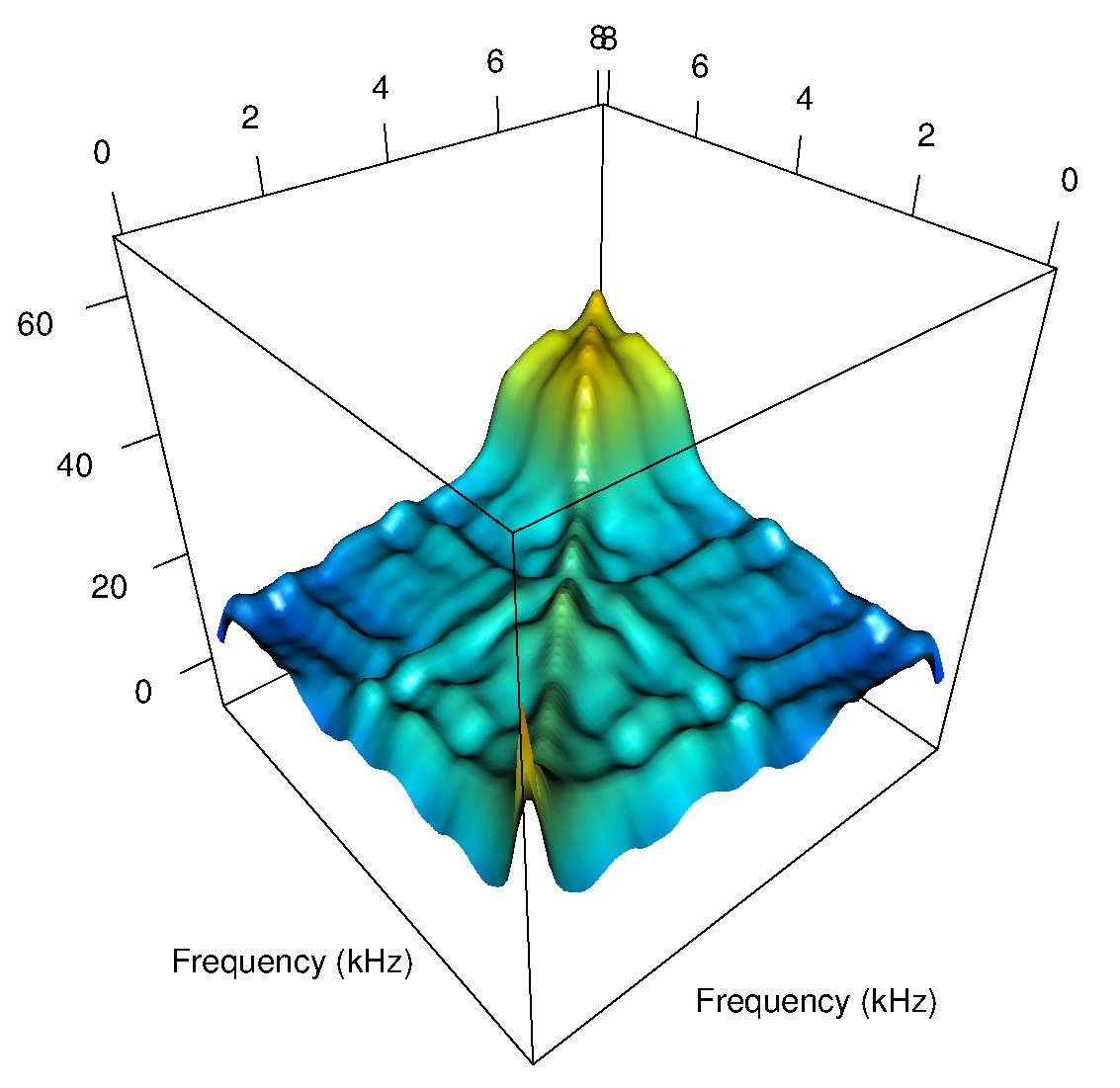
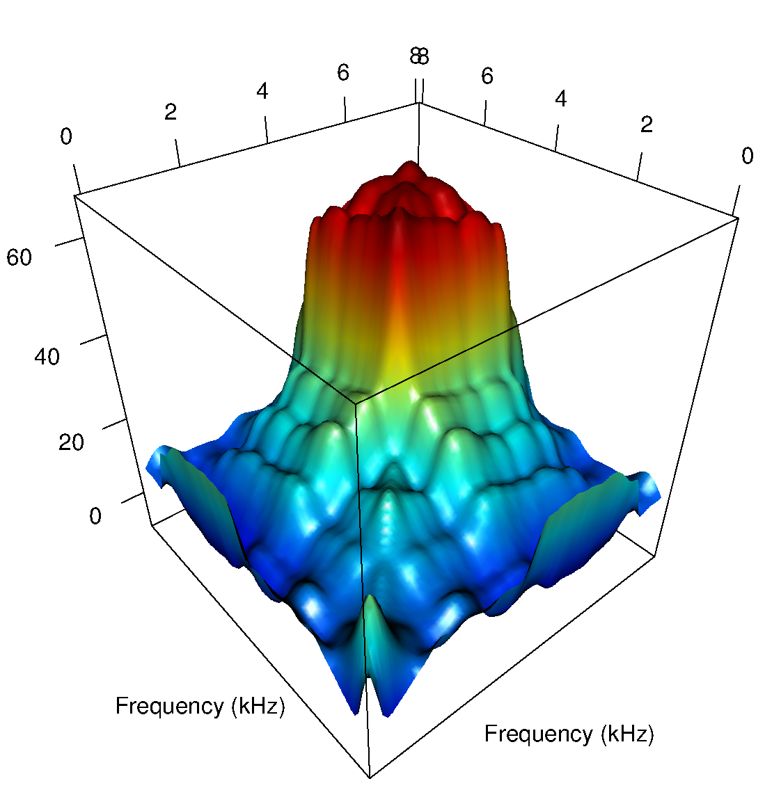
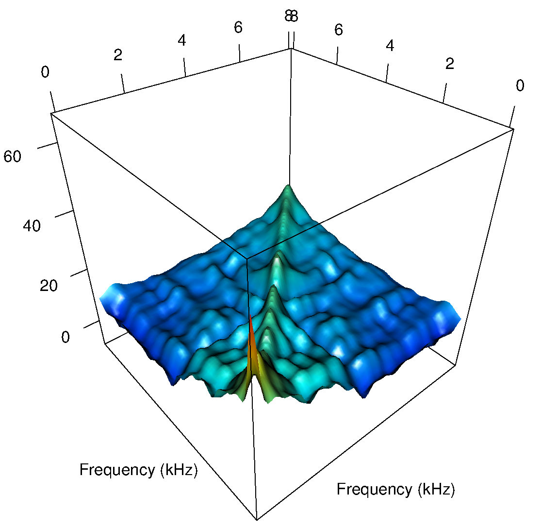
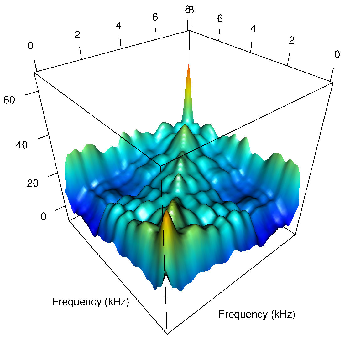
Figure 2: Marginal covariance function between frequencies for the five Romance languages. First row: Italian (left), French (center) and Portuguese (right). Second row: American Spanish (left) and Iberian Spanish (right).

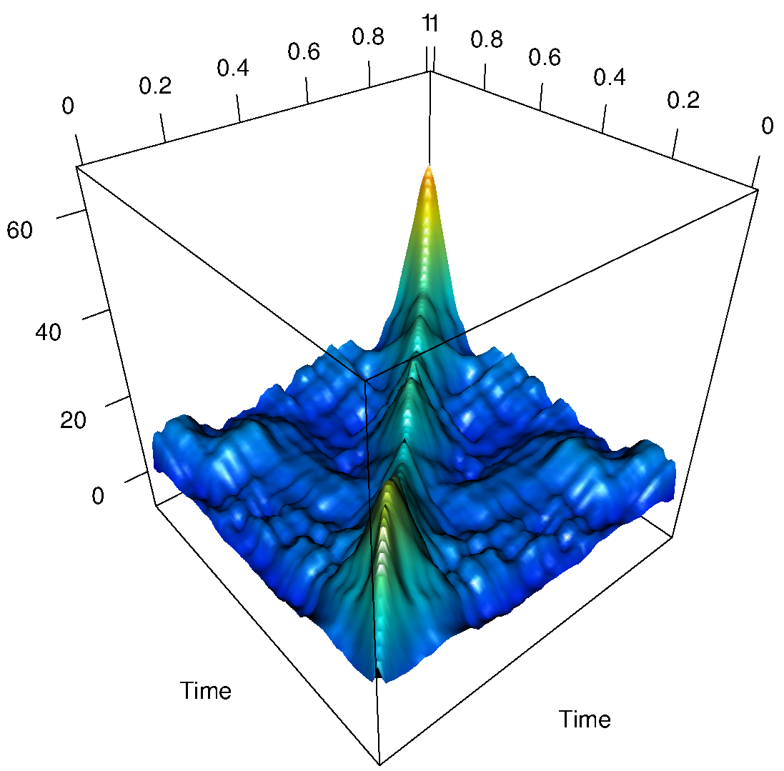
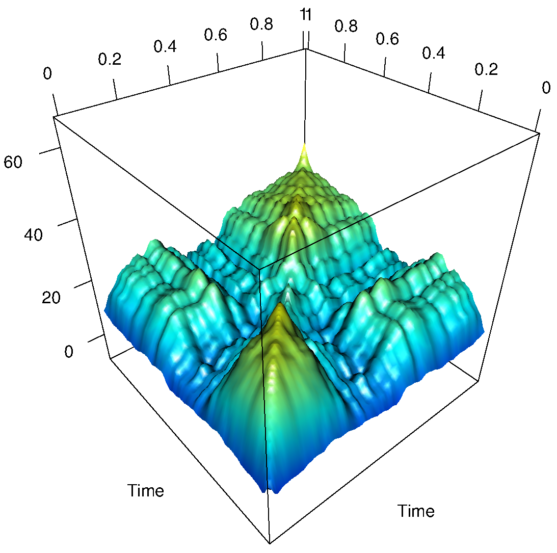
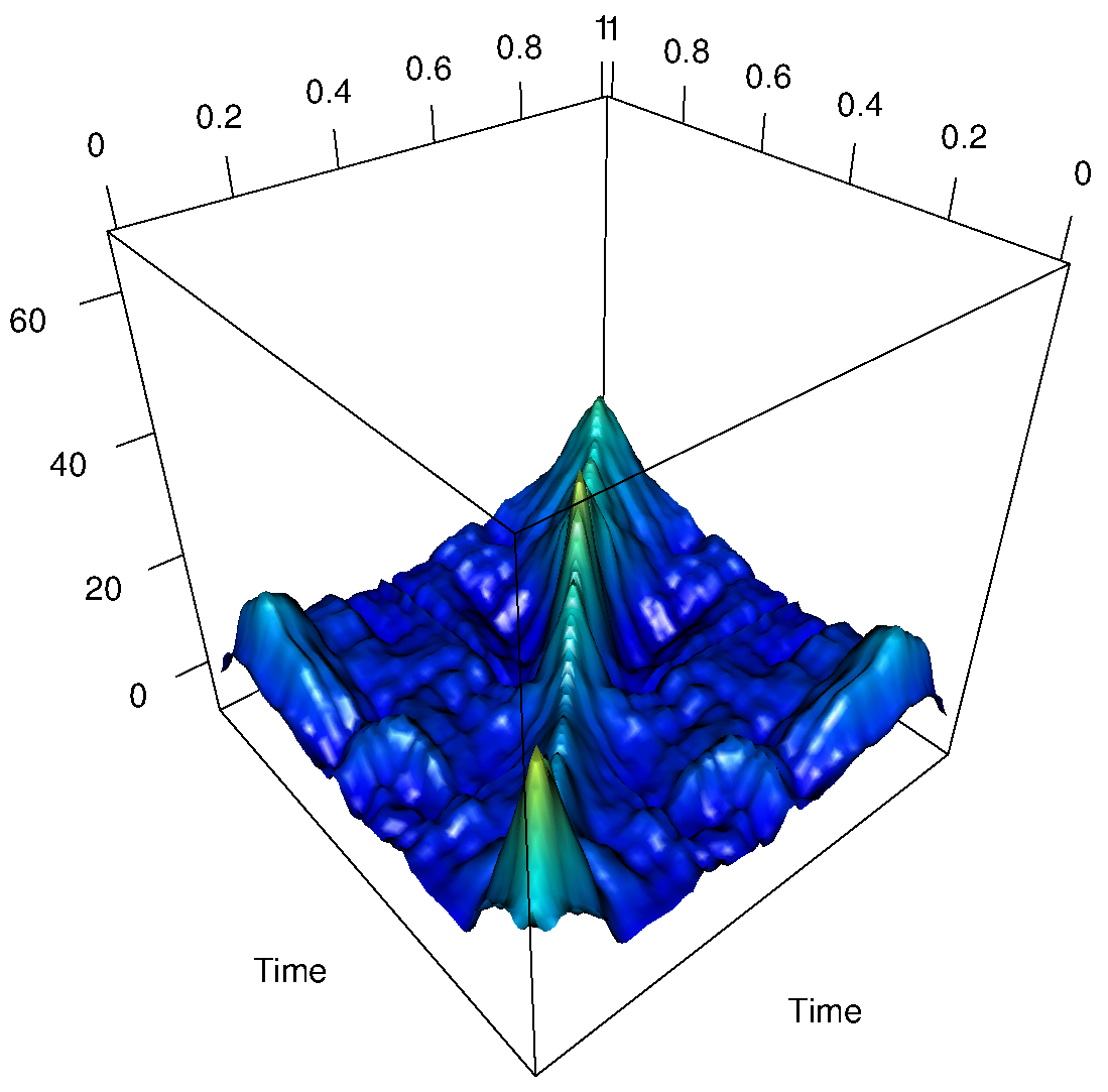
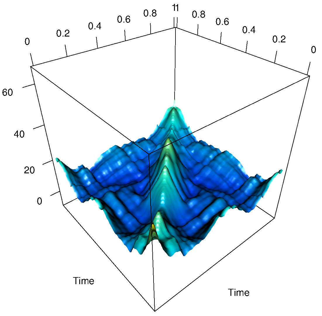
Figure 3: Marginal covariance function between times for the five Romance languages. First row: Italian (left), French (center) and Portuguese (right). Second row: American Spanish (left) and Iberian Spanish (right).

5.1 A permutation test to compare means and covariance operators between groups

We made the assumption above that the covariance operators are common to all the words within each language, while the means are different between words. This assumption can be verified using permutation tests that look at the effect of the group factor on the parameters of the sound process.

When an estimator for a parameter is available and it is possible to define a distance $d(.,.)$ between two estimates, a distance-based permutation test can be set up in the following way. Let $X_{1l},\ldots,X_{nl}$ be a sample of surfaces from the $l$-th group under consideration and $K_{l}=K(X_{1l},\ldots,X_{nl})$ be an estimator for an unknown parameter $\Gamma_{l}$ of the process which generates the data belonging to the $l$-th group. In the case of acoustic phonetic data, this parameter can be for example the mean, the frequency covariance operator or the time covariance operator.

Permutation tests are non parametric tests which rely on the fact that, if there is no difference among experimental groups, the group labelling of the observations (in our case the log-spectrograms) is completely arbitrary. Therefore, the null hypothesis that the labels are arbitrary is tested by comparing the test statistic with its permutation distribution, i.e. the value of the test statistics for all the possible permutation of labels. In practice, only a subset of permutations, chosen at random, is used to assess the distribution. A sufficient condition to apply this permutation procedure is exchangeability under the null hypothesis. This is trivially verified in the case of the test for the mean. For the comparison of covariance operators, this implies the groups having the same mean. If this not true, we can apply the procedure to the centred observations $\widetilde{X}_{il}=X_{il}-\overline{X}_{l}$, $i=1,\ldots,n$, $l=1,\ldots,G$, where $\overline{X}_{l}$ is the sample mean for the $l$-th group. This guarantees the observations to be asymptotically exchangeable due to the law of large numbers.

Indeed, if we want to test the null hypothesis that $\Gamma_{1}=\Gamma_{2}=\cdots=\Gamma_{G}$ against the alternative that the parameter is different for at least one group, we can consider as test statistic

$$T_{0}=\frac{1}{G}\sum_{l=1}^{G}d(K_{l},\overline{K})^{2},$$

where $\overline{K}$ is the sample Fréchet mean of $K_{1},\ldots,K_{G}$, defined as

$$\overline{K}=\arg\min_{K\in P}\frac{1}{G}\sum_{l=1}^{G}d(K_{l},K)^{2},$$

where $P$ is the appropriate functional space to which the parameters belong. This test statistic measures the variability of the estimator of the parameters across the different groups. If the parameter is indeed different for some groups, we expect that the their estimates from groups $1,\ldots,G$ show greater variability than those obtained from random permutations of the group labels in the data set. Thus, large values of $T_{0}$ are evidence against the null hypothesis.

Let us take $M$ permutations of the original group labels and compute the test statistic for the permuted sample $T_{m}=\sum_{l=1}^{G}d(K_{l}^{m},\overline{K}^{m})^{2}$, where $K_{l}^{m}$, $l=1,\ldots,G$ are the estimates of the parameters obtained from the observations assigned to the group $l$ in the $m$-th permutation and $\overline{K}^{m}$ is their sample Fréchet mean. The p-value of the test will therefore be the proportion of permutations for which the test statistic is greater than in the original data set, i.e. $p=\frac{\#\{T_{m}>T_{0}\}}{M}$.

We apply now this general procedure to the three parameters of interest in our case, i.e. the mean, the frequency covariance operator and the time covariance operator, when the groups are the different words within each language and/or the different language.

Let us start by considering the test to compare the means of the log-spectrograms across the words (digit) of each language. Here the natural estimator for the word-wise mean log-spectrogram is the sample mean, i.e.

$$K_{l}=\overline{S}_{l}^{L}(\omega,t)=\frac{1}{n_{l}}\sum_{k=1}^{n_{l}}S_{lk}^{L}(\omega,t)$$

and the distance can be chosen to be the distance in $L^{2}([0,8\ \mathrm{kHz}]\times[0,1])$,

$$d(\overline{S}_{l}^{L},\overline{S}_{l^{\prime}}^{L})=\sqrt{\int_{0}^{8\mathrm{kHz}}\int_{0}^{1}[\overline{S}_{l}^{L}(\omega,t)-\overline{S}_{l^{\prime}}^{L}(\omega,t)]^{2}\mathrm{d}\omega\mathrm{d}t}.$$

Table 1 reports the results for the test for the difference of the means between the digit $l=1,\ldots,10$ for the five Romance languages. It can be seen that a significant difference can be found for French and American Spanish and thus we choose to account for this difference when modelling the sound changes.

We can apply the same procedure to the test for the covariance operators. First, we need to define a distance between covariance operators. Pigoli et al., (2014) show that when the covariance operator is the object of interest for the statistical analysis, a distance-based approach can be fruitfully used and the choice of the distance is relevant, different distances catching different properties of the covariance structure. In particular, they propose a distance based on the geometrical properties of the space of covariance operators, the Procrustes reflection size-and-shape distance. This distance uses a map from the space of covariance operators to the space of Hilbert-Schmidt operators, i.e. compact operator with finite norm $||L||_{HS}=\mathrm{trace}(L_{i}^{*}L_{i})$. This being a Hilbert space, distances between the transformed operators can be easily evaluated. However, the map is defined up to a unitary operator and a Procrustes matching is therefore needed to evaluate the distance between the two equivalence classes. Let $C_{1}$ and $C_{2}$ be the covariance operators we want to compare and $L_{1}$ and $L_{2}$ the Hilbert-Schmidt operators such that $C_{i}=L_{i}L_{i}^{*}$. Pigoli et al., (2014) prove that the Procrustes reflection size-and-shape distance has the explicit analytic expression

$$d_{P}(C_{1},C_{2})^{2}=||L_{1}||_{HS}^{2}+||L_{2}||_{HS}^{2}-2\sum_{k=1}^{\infty}\sigma_{k},$$

where $\sigma_{k}$ are the the singular values of the compact operator $L_{2}^{*}L_{1}$. A possible map is the square root $L_{i}=(C_{i})^{1/2}$ (although the distance itself is invariant to the choice of map) and we use this choice in the following analysis, where we analyze the five selected Romance languages looking at the Procrustes distance between their frequency covariance operators.

For a given choice of the distance, a sample Fréchet mean and variance of a set of covariance operators $C^{1},\ldots,C^{L}$ can be defined as

$$\overline{C}=\arg\inf_{C}\sum_{L=1}^{G}d(C^{L},C)^{2},\hskip 28.45274pt\widehat{\sigma}^{2}=\frac{1}{G}\sum_{L=1}^{G}d(C^{L},\overline{C})^{2}.$$

These provide estimates for the centre point and the variability of the distribution with respect to the distance $d(.,.)$, which are needed for the test statistic in the permutation test.

Table 1: P-values of the permutation tests for H$0$: $\mu_{1}^{L}=\mu_{2}^{L}=\cdots=\mu_{10}^{L}$ vs H$1$: at least one is different, where $\mu_{i}^{L}$ is the mean log-spectrogram for the language $L$ and word $i$, for the five Romance languages.

Language	French	Italian	Portuguese	American Spanish	Iberian Spanish
$p-value$	$<$0.001	0.02	0.96	$<$0.001	0.205

Table 2: P-values of the permutation tests for H$0$: $C_{\omega,1}^{L}=C_{\omega,2}^{L}=\cdots=C_{\omega,10}^{L}$ vs H$1$: at least one is different, where $C_{\omega,i}^{L}$ is the marginal frequency covariance operator for the language $L$ and word $i$, for the five Romance languages. The Procrustes distance is used for the test statistic.

Language	French	Italian	Portuguese	American Spanish	Iberian Spanish
$p-value$	0.113	0.991	0.968	0.815	0.985

Table 3: P-values of the permutation tests for H$0$: $C^{L}_{t,1}=C^{L}_{t,2}=\cdots=C^{L}_{t,10}$ vs H$1$: at least one is different, where $C_{t,i}^{L}$ is the marginal time covariance operator for the language $L$ and word $i$, for the five Romance languages. The Procrustes distance is used for the test statistic.

Language	French	Italian	Portuguese	American Spanish	Iberian Spanish
$p-value$	0.02	0.422	0.834	0.683	0.17

Using this procedure, we can verify whether the assumption that the covariance operators are the same across the words is disproved by the data. Table 2 shows the p-values of the permutation tests for the equality of the marginal frequency covariance operator across the different words for the five Romance languages described in Section 2, obtained with the Procrustes distance between sample covariance operators and $M=1000$ permutations on the residual log-spectrograms. In the interpretation of these p-values, we need to account for the multiple tests that have been carried out. By applying a Bonferroni correction to the p-values in Table 2, it can be seen that there is no evidence against the hypothesis that the covariance operator is the same for all words for all the considered languages. The same is true for the time covariance operator, as can be seen in Table 3, which reports the unadjusted p-values of this second test.

A possible concern is that the dimension of the data set becomes relatively small when it is split between the different words and language and therefore these testing procedure will have little power. On the other hand, this reasoning encourages us to simplify the model (assuming covariance operators constant across words) so that enough observations are available to estimate the parameters accurately. With a larger data set that allows us to highlight differences between word-wise covariance operators, we would have more information to estimate these operators accurately.

6 Exploring phonetic differences

We now have the tools to explore the phonetic differences between the languages in the Oxford Romance languages data set. This can be done at different levels. A possible way to go would be to pair two speakers belonging to two different languages and look at their difference. However, this neglects the variability of the speech within the language and it would not be clear which aspects of the phonetic differences are to be credited to the difference between languages and which to the difference between the two individual speakers, unless we had available recordings from bilingual subjects. In this section we present a possible approach to the modelling of phonetic changes that takes into account the features of the speaker's population.

6.1 Modelling changes in the parameters of the phonetic process

We can start by looking at the path that links the mean of the log-spectrograms between two words of different languages. These should be two words known to be related in the languages' historical development. This is the case for example for the same digit in any two different Romance languages.

Considered as functional objects, the log-spectrograms means are unconstrained and integrable surfaces, thus interpolation and extrapolation can be simply obtained with a linear combination, where the weights are determined from the distance of the language we want to predict from the known languages. For example, if we want to reconstruct the path of the mean for the digit $i$ from the language $L_{1}$ to the language $L_{2}$, we have

$$\overline{S}_{i}(x)=\overline{S}_{i}^{L_{1}}+x(\overline{S}_{i}^{L_{2}}-\overline{S}_{i}^{L_{1}}),$$

where $x\in[0,1]$ provides a linear interpolation from language $L_{1}$ to language $L_{2}$, while $x<0$ or $x>1$ provides an extrapolation in the direction of the difference between the two languages, with $\overline{S}_{i}^{L}$ being the mean of the log-spectrograms from speakers of the language $L$ pronouncing the $i$-th digit. For example, Figure 9 shows six steps along a reconstructed path for the mean log-spectrogram of ``one'', from French [œ̃] to Portuguese [ũ]. Indeed, this path has historical significance, as the sound change from Latin ``unus'' to French ``un'' likely went via the sound [ũ], which is still maintained in modern Portuguese (it should be noted that we are, of course, not implying that modern French is derived from Portuguese, but merely that a historical sound of modern French is maintained in Portuguese).

A natural question is whether this can replicated for the covariance structure, in order to interpolate and extrapolate a more general description of the sound generation process. However, the case of the covariance structure is more complex. Experience with low dimensional covariance matrices (see Dryden et al.,, 2009) and the case of the frequency covariance operators illustrated in Pigoli et al., (2014) show that a linear interpolation is not a good choice for objects belonging to a non-Euclidean space. We want therefore to use a geodesic interpolation based on an appropriate metric for the covariance operator. Moreover, since we model the covariance structure as separable, we also want the predicted covariance structure to preserve this property. It is not possible to do this with geodesic paths in the general space of four-dimensional covariance structures and thus we define the new covariance structure as the tensor product of the geodesic interpolations (or extrapolations) in the space of time and frequency covariance operators,

$$C^{x}=C_{\omega}^{x}\otimes C_{t}^{x},$$

where the geodesic interpolations (or extrapolations) $C_{\omega}^{x}$, $C_{t}^{x}$ depend on the chosen metric. In the case of the Procrustes reflection size and shape distance, the geodesic has the form

$$C_{r}^{x}=[(C_{r}^{L_{1}})^{1/2}+x((C_{r}^{L_{2}})^{1/2}\widetilde{R}-(C_{r}^{L_{1}})^{1/2})][(C_{r}^{L_{1}})^{1/2}+x((C_{r}^{L_{2}})^{1/2}\widetilde{R}-(C_{r}^{L_{1}})^{1/2})]^{*}$$

where $r=\omega,t$ and $\widetilde{R}$ is the unitary operator that minimizes $||(C_{r}^{L_{1}})^{1/2}-(C_{r}^{L_{2}})^{1/2}R||^{2}_{HS}$ (see Pigoli et al.,, 2014). Other choices of the metric are of course possible, as long as they provide a valid geodesic for the covariance operator. However, some preliminary experiments reported in Pigoli et al., (2014) suggest that the Procrustes reflection size and shape geodesic performs better in the extrapolation of frequency covariance operators than existing alternatives.

6.2 What would someone sound like speaking in a different language?

The framework we have set up allows us also to observe how the sound produced by a speaker would be modified as we move to a different language. As mentioned in the introduction, we aim to map the sound produced by this speaker to that of a hypothetical speaker with the same position in the space of possible speakers in a different language, with respect to the language variability structure. To do this, we need some additional specification of the statistical model which generates the log-spectrograms. For example, if we assume that the log-spectrograms of a spoken word are generated from a Gaussian process, its distribution is fully determined by the mean log-spectrogram (which is expected to be word-dependent) and the covariance structure. More generally, we identify the population of possible pronunciations of a specific word of a language through its mean log-spectrogram, which is word-specific, and its time and frequency covariance functions, which are properties of the whole language. Thus, we identify as a speaker-specific residual what is left in the phonetic data once means and covariance information have been removed. Let us denote with $\mathfrak{F}_{i}^{L}$ this operation for the word $i$ of the language $L$. Then, we can obtain a representation of the log-spectrogram for a speaker from a language $L_{1}$ in the language $L_{2}$ as

$$S_{ik}^{L_{1}\rightarrow L_{2}}=[\mathfrak{F}_{i}^{L_{2}}]^{-1}\circ\mathfrak{F}_{i}^{L_{1}}(S_{ik}^{L_{1}}).$$ (3)

We choose to use the same word for both languages because in our data set words can be paired in a sensible way (the various pronunciations of the same digit in two Romance languages sharing a common historical origin).

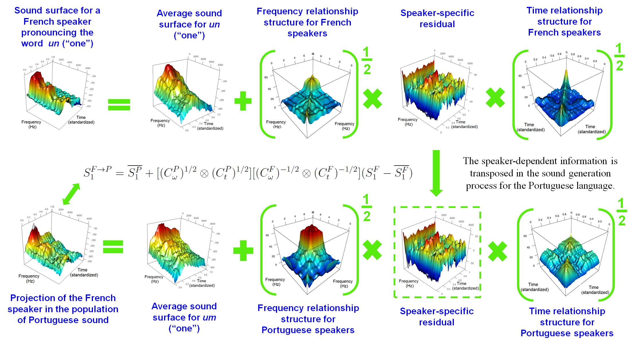
Figure 4: Example of the mapping of a French speaker's log-spectrogram to the same position in the space of Portuguese pronunciations fo the corresponding word.

The challenge now is how to define the transformation $\mathfrak{F}_{i}^{L}$. This is obtained considering both the characteristics of the sound populations in the two languages and the relative ``position'' of the speaker in their language vis-a-vis all the other speakers. A graphical representation of this idea for the case of a French speaker mapped to the Portuguese language can be seen in Fig. 4. To define this transformation, we start from a speaker $k$ from the language $L_{1}$ and we consider the residual log-spectrogram $R_{ik}^{L_{1}}=S_{ik}^{L_{1}}-\overline{S}_{i.}^{L_{1}}$. We would like to apply now a transformation that makes this residual uncorrelated, as generated by a white noise process. Let us consider the transformation from a finite dimensional white noise

$$Z=\sum_{i,j}^{p}z_{ij}v_{i}^{\omega}\otimes v^{t}_{j},\hskip 14.22636ptz_{ij}\sim N(0,1)$$

to a random surface with the same mean and covariance structure $(C^{L_{1}}_{\omega})^{1/2}_{1}\otimes(C^{L_{1}}_{t})^{1/2}Z$ of the sound distribution. We use here the notation for the application of a tensorised operator where

$$L_{1}\otimes L_{2}Z(\omega,t)=\int\int l_{1}(\omega,y)z(x,y)l_{2}(x,t)\mathrm{d}x\mathrm{d}y.$$

To obtain $\mathfrak{F}_{i}^{L}$, we would need to invert the transformation from $Z$ to the sound process. This is not possible in general (due to the unbounded nature of inverse covariance operators), but we can restrict the inverse to work on the subspaces spanned by our data, thus defining $(C^{L}_{l})^{-1/2}=\sum_{j=1}^{N}(\lambda_{j})^{-1/2}\phi_{j}\otimes\phi_{j}$, $\phi_{j},j=1,\ldots,N$, $\{\lambda_{j},\phi_{j}\}$ being eigenvalues and eigenfunctions for $C^{L}_{l}$. We then obtain

$$\mathfrak{F}_{i}^{L}(S_{ik}^{L})=(C^{L}_{\omega})^{-1/2}\otimes(C^{L}_{t})^{-1/2}(S_{ik}^{L}-\overline{S}_{i.}^{L})$$

and

$$[\mathfrak{F}_{i}^{L}]^{-1}(Z)=(C^{L}_{\omega})^{1/2}\otimes(C^{L}_{t})^{1/2}Z+\overline{S}_{i.}^{L}.$$

Figure 5 shows the log-spectrograms for the word un (``one'') of the first French speaker $S_{11}^{Fr}$, its representation when mapped to Portuguese um (``one'') $S_{11}^{Fr\rightarrow P}$ and the closest observed instance of Portuguese um as spoken by a Portuguese speaker, while Fig. 6 reports the result of the same operation applied to an Italian speaker, transforming Italian uno (``one'') into Iberian Spanish uno (``one''). Though the spelling is the same in this case, the pronunciation of the word in the two languages is not identical, albeit similar.

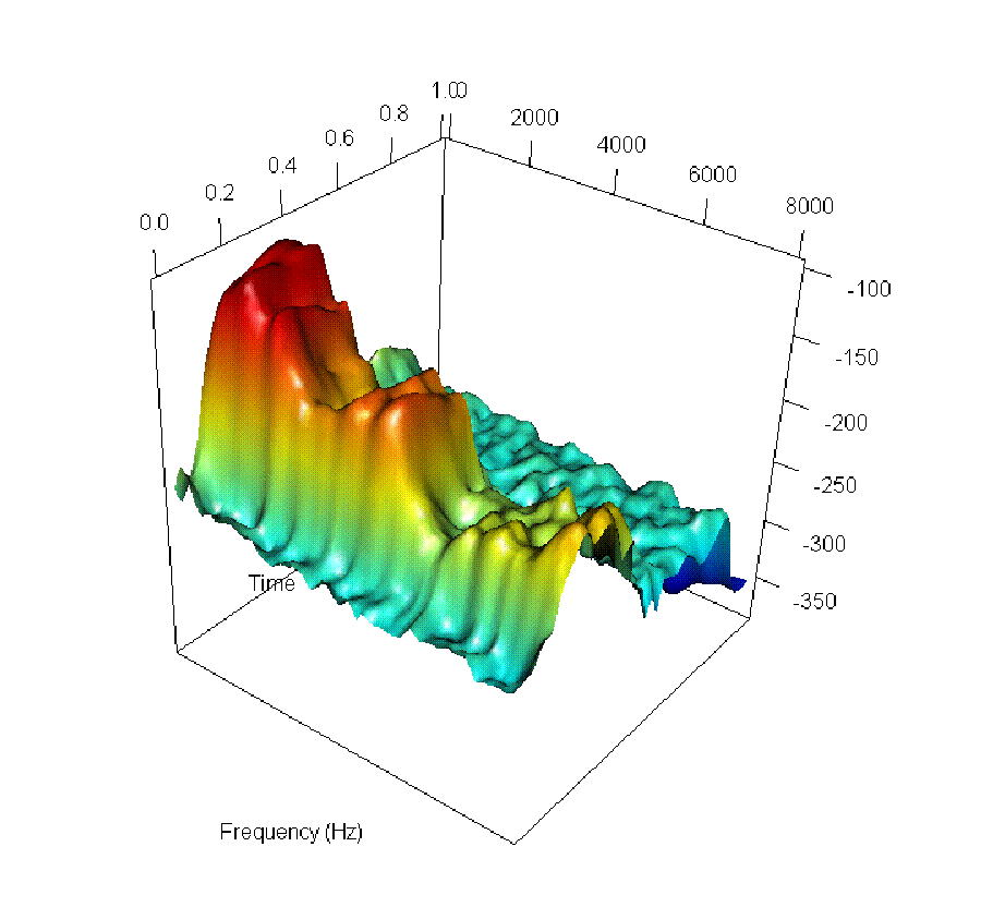
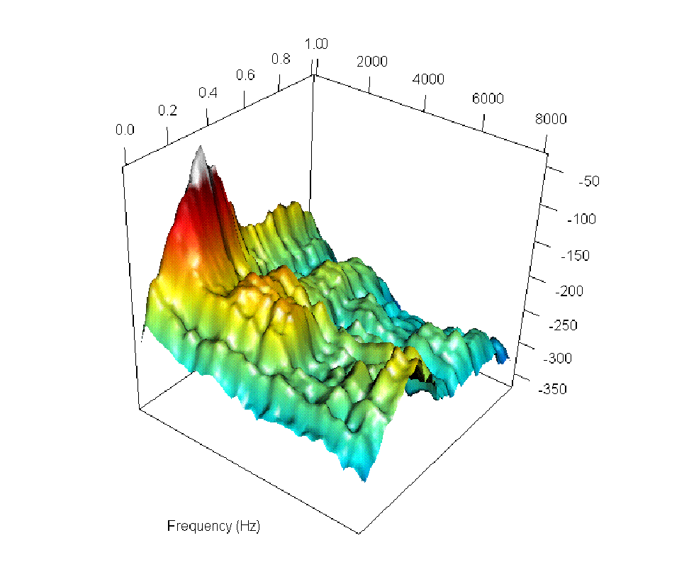
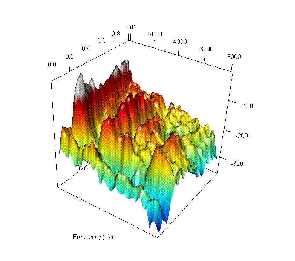
Figure 5: Log-spectrograms for the word un (``one'') as spoken by a French speaker (left), its representation as word um (``one'') in Portuguese using equation (3) (center) and the closest observed word um (``one'') spoken by a Portuguese speaker.

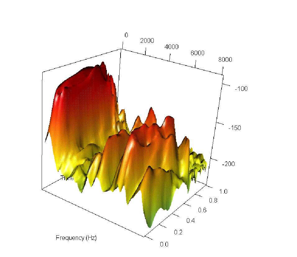
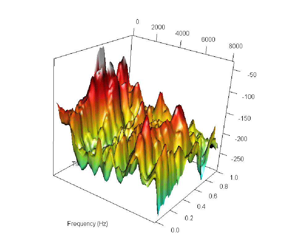
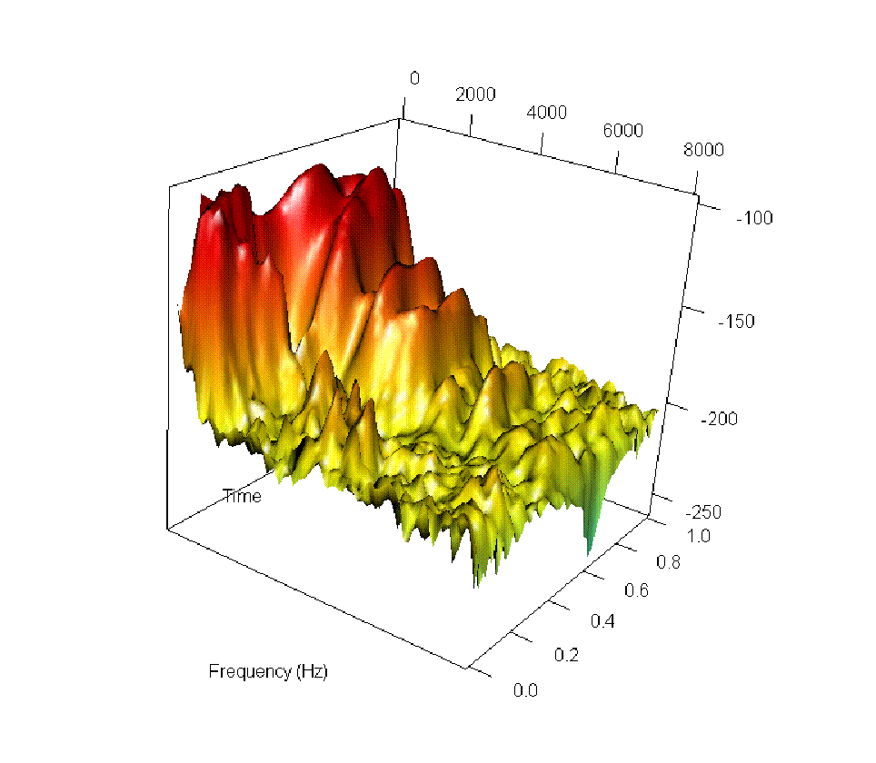
Figure 6: Log-spectrograms for the word uno (``one'') as spoken by an Italian speaker (left), its representation as word uno (``one'') in Spanish using equation (3) (center) and the closest observed word uno (``one'') spoken by a Spanish speaker.

6.3 Interpolation and extrapolation of spoken phonemes

The representation of a speaker as they would sound when speaking another language is interesting but is not enough for scholars to explore the historical sequence of changes that occurred between two languages: a smooth estimate of the path of change is needed. This is also the case if it is desired to extrapolate the sound transformation process beyond the path connecting the two languages, which we recall is a main goal of the Ancient Sounds project. Luckily, we can use the interpolated means and covariance operators described above to characterize the unobserved possible languages that are the intermediate steps in the phonetic path between two given languages. We thus obtain a smooth path between $S_{ik}^{L_{1}}$ and its representation in the language $L_{2}$ as

$$S_{ik}^{L_{1}\rightarrow L_{2}}(x)=[\mathfrak{F}_{i}^{x}]^{-1}\circ\mathfrak{F}_{i}^{L_{1}}(S_{ik}^{L_{1}}),$$ (4)

$[\mathfrak{F}_{i}^{x}]^{-1}=(C_{\omega}(x))^{1/2}\otimes(C_{t}(x))^{1/2}Z+M(x)$, where $C_{\omega}(x)$ is the interpolated (or extrapolated) frequency covariance operator, $C_{t}(x)$ the correspondent time covariance operator and $M(x)$ the word-dependent mean. An example of a smooth path between the log-spectrogram for the word un as spoken by the same French speaker considered in the previous section and its corresponding acoustic representation in Portuguese can be seen in Fig. 7.

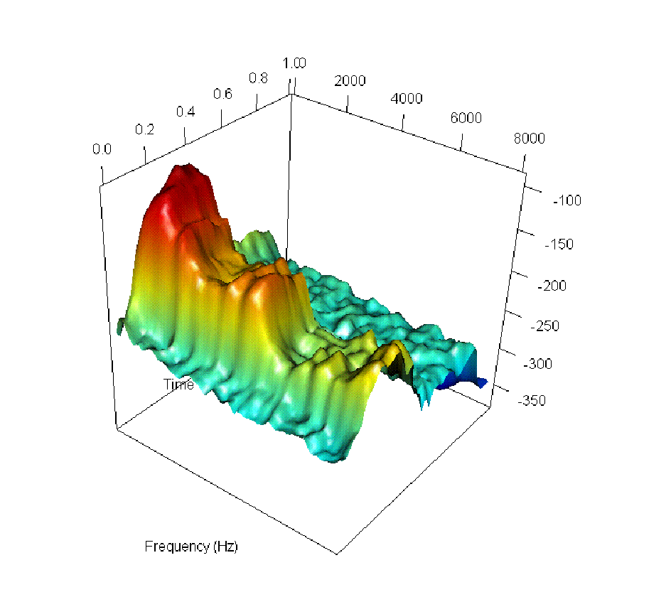
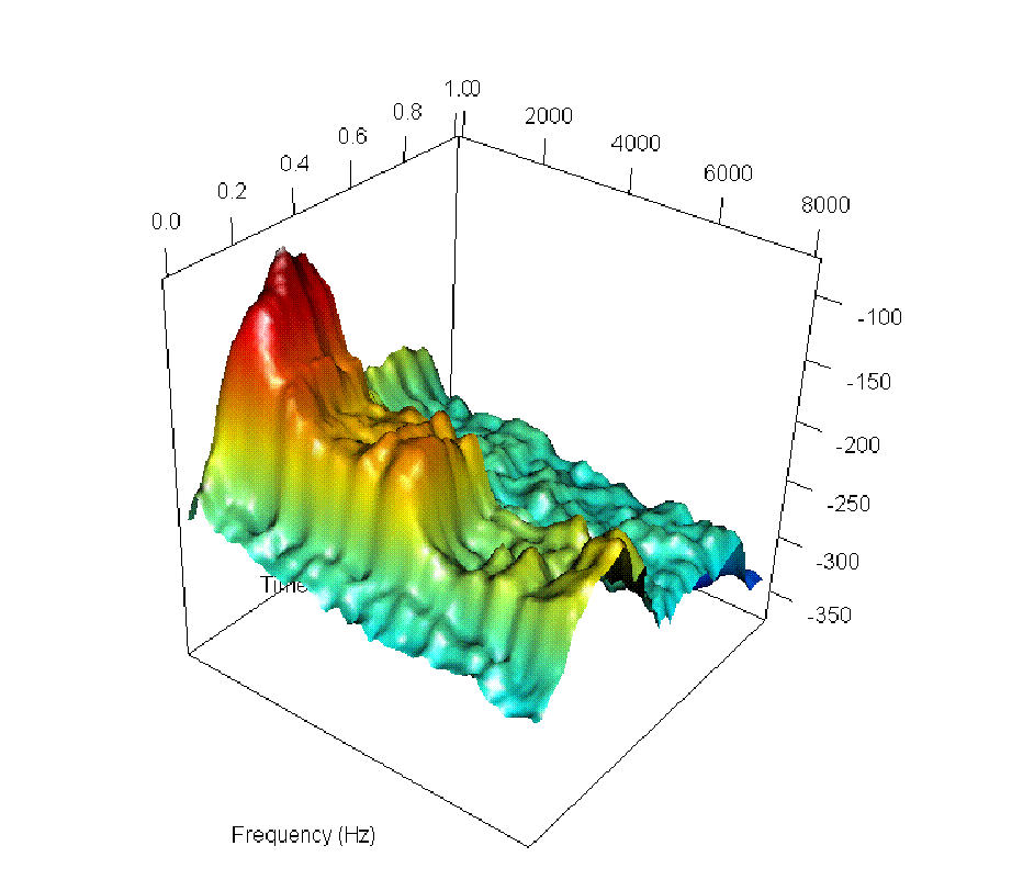
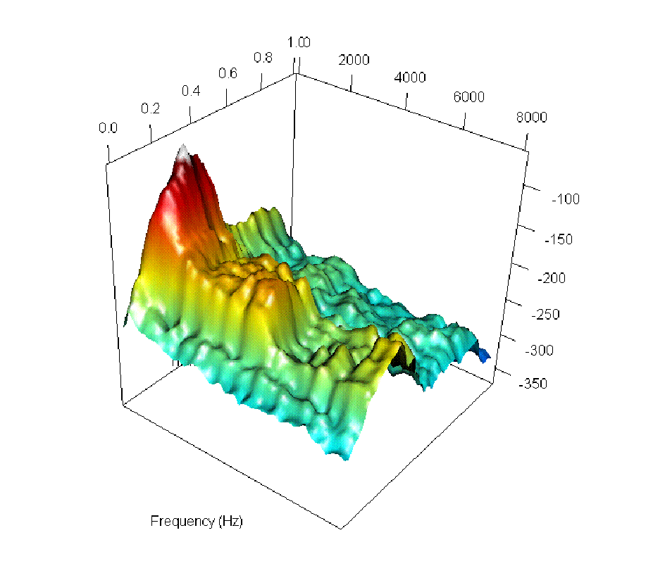
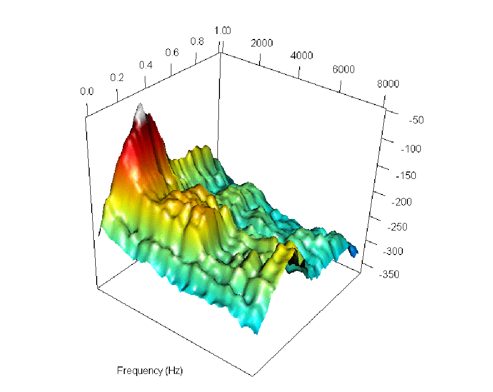
Figure 7: Six steps along the smooth path between the log-spectrogram for the word un (``one'') as spoken by a French speaker (top left) and its representation in Portuguese (bottom right).

This strategy can also be used to reconstruct a smooth path between two observed log-spectrograms $S_{ik}^{L_{1}}$ and $S_{ik^{\prime}}^{L_{2}}$, in this case the path being

$$S_{ik\rightarrow{ik^{\prime}}}^{L_{1}\rightarrow L_{2}}(x)=[\mathfrak{F}_{i}^{x}]^{-1}(x\mathfrak{F}_{i}^{L_{1}}(S_{ik}^{L_{1}})+(1-x)\mathfrak{F}_{i}^{L_{2}}(S_{i{k^{\prime}}}^{L_{2}})),$$ (5)

where a linear interpolation between the residuals takes the place of the residual of the single language. This could be useful when it is meaningful to pair two log-spectrograms in different languages, for example because the same speaker is recorded in two languages. This is not the case in our data set, but by way of example we report in Fig. 8 the path between the log-spectrograms for the word un for a French speaker $S_{11}^{Fr}$ and the word um for the Portuguese speaker who is closest to the transformed $S_{11}^{Fr\rightarrow P}$. It is also interesting to compare this with the interpolated path between the two mean log-spectrograms in Fig. 9.

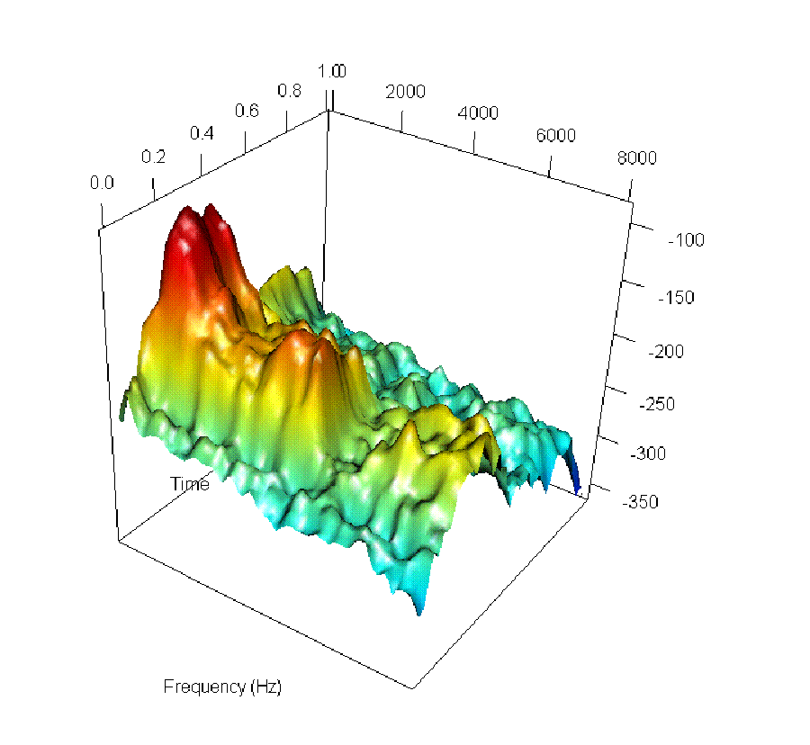
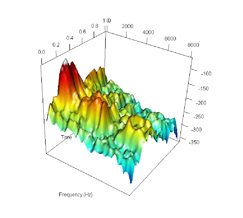
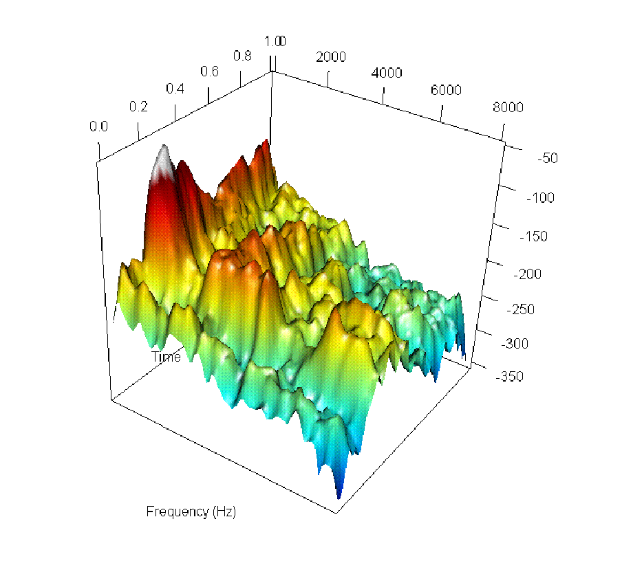
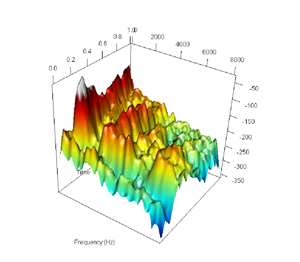
Figure 8: Six steps along the smooth path between the log-spectrograms for the word un (``one'') as spoken by a French speaker (top left) and the one for the word um (``one'') closest to its transformed representation in Portuguese (bottom right).

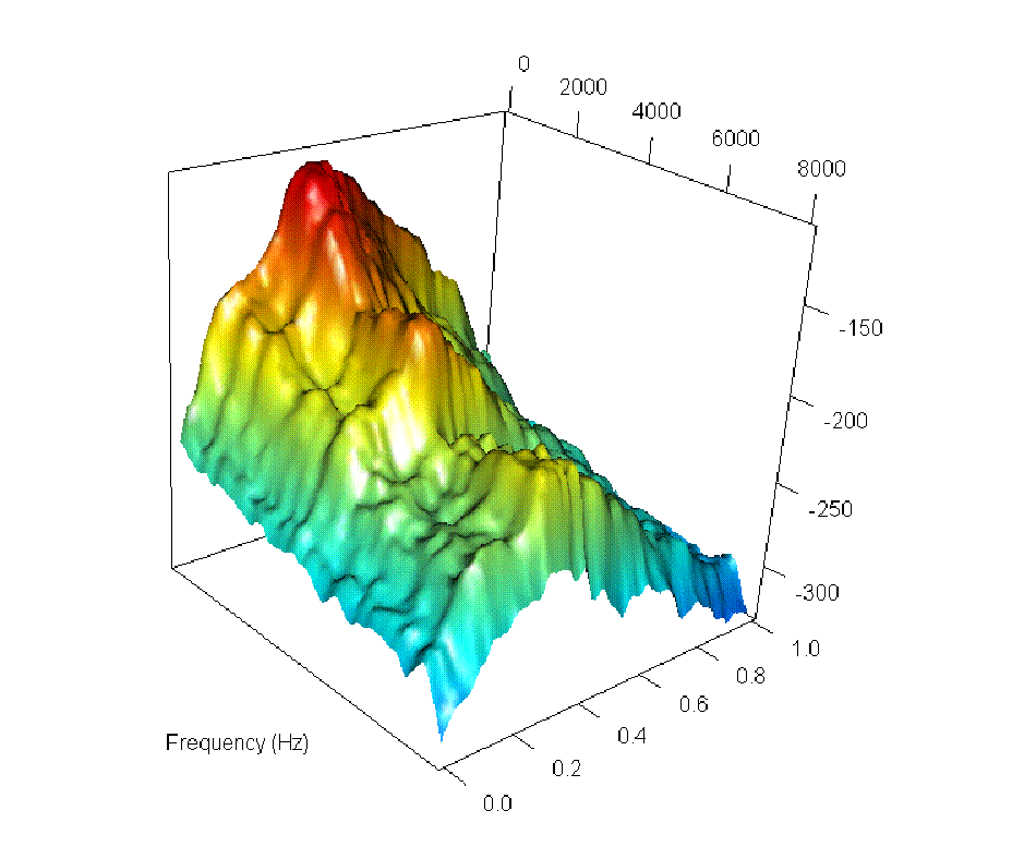
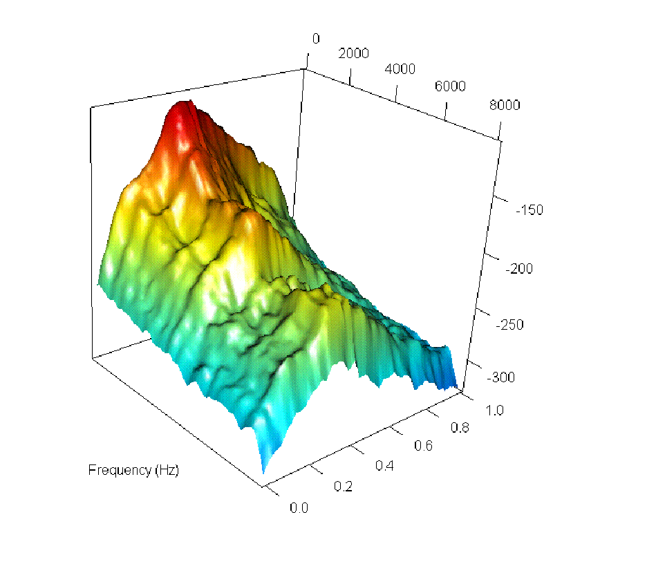
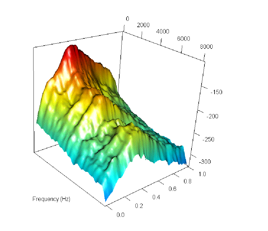
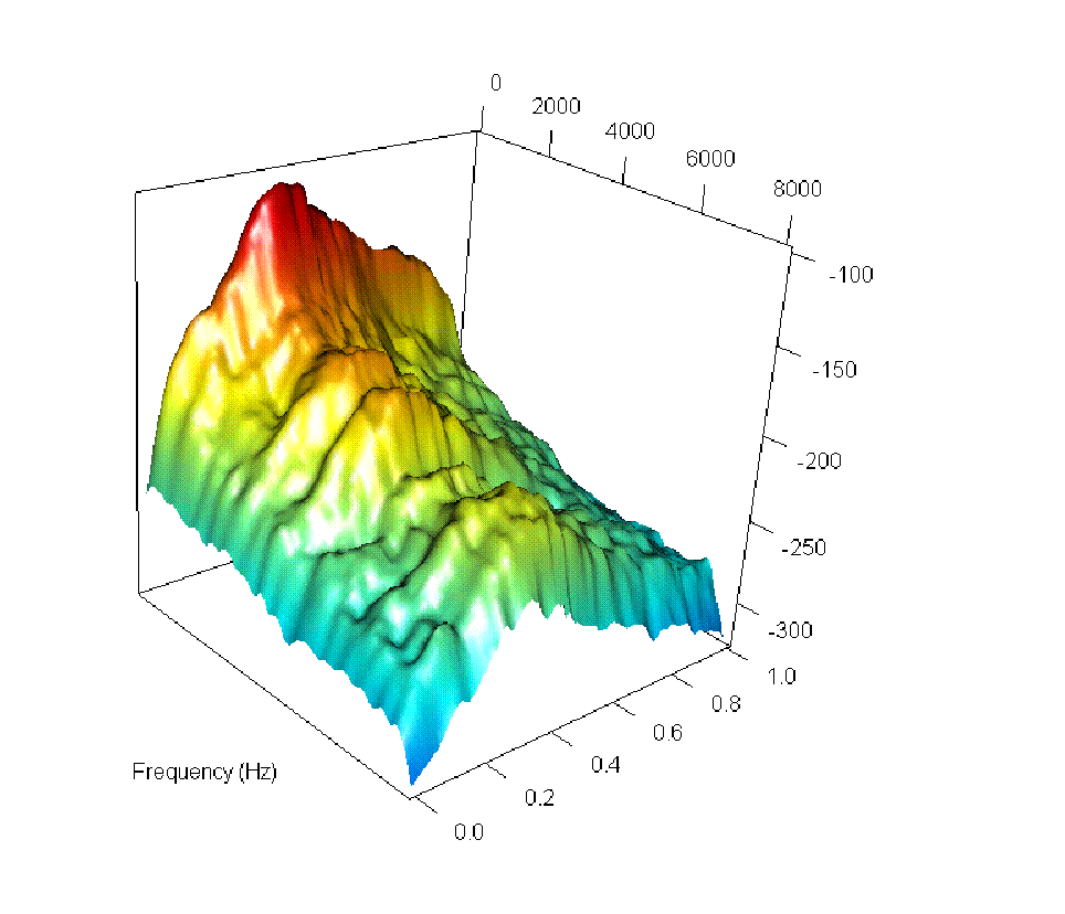
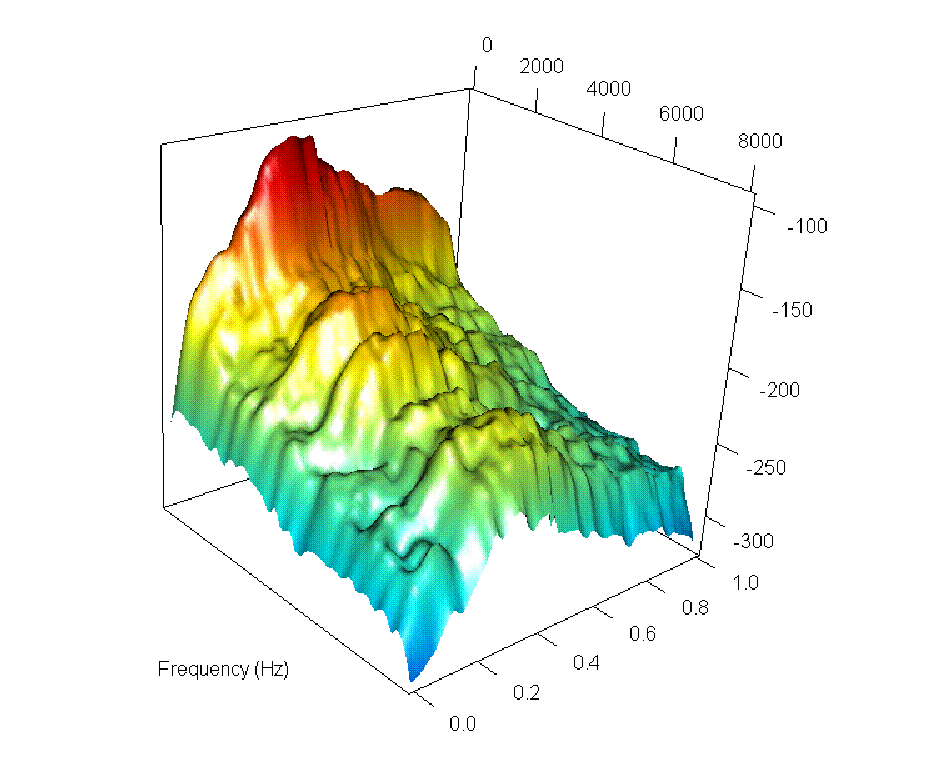
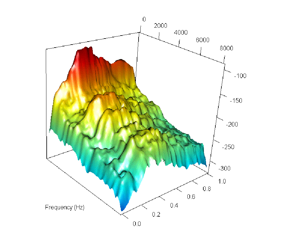
Figure 9: Six steps along the smooth path $M(x)$ between the mean log-spectrogram for the word un (``one'') in French (top left) and the one for the word um (``one'') in Portuguese (bottom right).

Being able to extrapolate the sounds opens up interesting possibilities whenever two languages are known to be at two stages of an evolutionary path. In this case extrapolating in the direction of the older (i.e. linguistically more conservative) language can provide an insight into the phonetic characteristics of the extinct ancestor languages. This, of course, will require some integration into a model of sound change with such information as that coming for example from textual analysis, history or archaeology (e.g. dating studies) . This is also needed as the rate of change of languages is not constant and the path $S^{L_{1}\rightarrow L_{2}}(x)$ can be travelled at different speed for different branches of the language family's evolution, and it can be changed by events such as conquests, migrations, language contact, etc. However, by having a path in the first place, addressing such questions is now a possibility.

6.4 Back to sound reproduction

Visualizing the log-spectrograms (or other transformation of the recorded sounds) is helpful but it is also important to listen to the signals in the original domain. This is also true for the representation of a sound in a different language and the smooth paths we have defined. Thus, we would like to reconstruct actual audible sounds from the estimated log-spectrograms. To do this, we would also need information about the phase component that we have so far disregarded, since we have focused all our attention on the amplitude component of the Fourier Transform (see Section 2). In principle, we could perform a parallel analysis on the phases to obtain representation of phase in a different language, the smooth path between phases and so on. However, this is tricky from a mathematical point of view, given the angular nature of the phases, and in any case there is no reason to believe there is additional information captured by phase (human hearing is largely insensitive to phase so it is quite normal practice in acoustic phonetics to disregard the phase component). In practice, we use the phase associated with the log-spectrogram $S_{ik}^{L_{1}}$ to reconstruct the sounds over the smooth path; the results are quite satisfactory. As supplementary material, some examples of reconstructed sound path can be provided.

7 Discussion

We have introduced a novel way to explore phonetic differences and changes between languages that takes into account the characteristics of the sound population on the basis of actual speech recordings. The framework we introduced is useful for dealing with acoustic phonetic data, i.e. samples of sound recordings of different words or other linguistic units from different groups (in our case, languages). We illustrate the proposed method with an application to a Romance digit data set, which includes the words corresponding to the numbers from one to ten pronounced by speakers of five different Romance languages. In particular, we verify in this data set the assumption that the covariance structure in the log-spectrograms is common for the different words within the language, thus increasing the sample available for its estimation. This is an interesting example of how the characteristics of a population (in this case the speakers of one language) may be captured in the second order structure and not only in the mean level. This in itself provides interesting information to linguists as it captures the notion of ``the sound of a language''. It also fits within the recent development of object oriented data analysis (see Wang and Marron,, 2007), which advocates a careful consideration of the object of interest for a statistical analysis. Here it seems that marginal covariance operators are promising features to represent phonetic structure at the level of a language.

We do not focus here on the representativeness or otherwise of the sample of speakers or words in the dataset. In view of a broad use of this approach however, it is important to remember that the sample of speakers should reflect the population we are interested in and in particular careful consideration should be given to regional and social stratification in the data set. Moreover, to speak properly of a ``language'' (and not just of a small subset of words), the words considered should be representative of the whole language. The digits studied here do contain a wide ranging set of different vowels and consonant (for just a few words), indicating that the results are likely to be generalisable to some extent across a larger corpus, but, of course, applying this to a much more comprehensive corpus of several languages would be advisable.

The proposed approach, using audio recordings in place of textual representations, allows us to account for the differences between different varieties of the same language, such as Castilian Spanish and American Spanish (Penny,, 2000). Moreover, recent works (see The Functional Phylogenies Group,, 2012; Bouchard-Côté et al.,, 2013; Coleman et al.,, 2015, and references therein) focus on the reconstruction of the distribution of phonetic features for ancestor languages. While the research in this field is still in its very earliest stages, as a better understanding of the historical evolution of sounds becomes available, this can be integrated into our methods to provide a reconstruction of how the speakers of extinct languages might have sounded. The final goal is therefore to integrate the modelling of the variability of speech within the language provided by our approach with the dynamics of sound change established by other researches both in linguistics and in statistics. We are confident that this will make a substantial contribution to the ongoing project whose goal is audible reconstruction of words in the proto-languages.

We have illustrated the transformation of a speaker's speech from one language to another as a first example application in speech generation but other problems can be addressed in this framework. For example, the proposed approach to model sound processes can be extended to take into account discrete or continuous covariates associated to the mean and the covariance operators. These can be seen as function of the geographical coordinates or of time-depth when studying dialects. While we treated the language as a categorical variable, nothing prevents us seeing it as a continuous process in space and time. Indeed, the definition of the continuous path between two languages described in Section 6.3 can be seen as the first step in this direction, since the abscissa $x$ of the path can be made dependent on external variables. While we do not claim this can straightforwardly reproduce the evolutionary branches in language history, it can still be a useful starting point for more complex models.

The application of the proposed method is not necessarily restricted to comparative linguistics. It can be useful whenever a comparison between groups of sounds is needed, or indeed other complex wavelike signals. In the future it will be interesting to explore micro-variation within a language (dialects, spoken language in different subgroups of the population) but also other types of sounds such as songs or even sounds different from human speech, for example animal calls.

Supplementary Material

Supplementary material is available on request from the corresponding author.

References

- Aston et al., (2010) Aston, J. A. D., Chiou, J.-M. and Evans, J. P. (2010) ``Linguistic Pitch Analysis using Functional Principal Component Mixed Effect Models'', Journal of the Royal Statistical Society Series C - Applied Statistics, 59, 297–317.
- Bouchard-Côté et al., (2013) Bouchard-Côté, A., Hall, D., Griffiths, T. L. and Klein, D. (2013) ``Automated reconstruction of ancient languages using probabilistic models of sound change'', Proceedings of the National Academy of Sciences, 110, 4224–4229.
- Cavalli-Sforza, (1997) Cavalli-Sforza, L. L. (1997) ``Genes, peoples, and languages'', Proceedings of the National Academy of Sciences, 94, 7719–7724.
- Coleman et al., (2015) Coleman, J., Aston, J. and Pigoli, D. (2015). ``Reconstructing the sounds of words from the past'', In The Scottish Consortium for ICPhS(Ed.) Proceedings of the 18th International Congress of Phonetic Sciences, Glasgow, UK.
- Cooke at al., (1993) Cooke, M., Beet, S. and Crawford, M. (1993) Visual representations of speech signals, John Wiley & Sons, Inc..
- Dryden and Mardia, (1998) Dryden, I. L. and Mardia, K. V. (1998) Statistical Shape Analysis. Wiley, Chichester.
- Dryden et al., (2009) Dryden, I. L., Koloydenko, A., Zhou, D. (2009), Non-Euclidean statistics for covariance matrices, with applications to diffusion tensor imaging, Annals of Applied Statistics, 3, 1102–1123.
- Ferraty and Vieu, (2006) Ferraty, F. and Vieu, P. (2006) Nonparametric Functional Data Analysis: Theory and Practice, Springer, Berlin.
- Garcia, (2010) Garcia, D. (2010) ``Robust smoothing of gridded data in one and higher dimensions with missing values'', Computational Statistics & Data Analysis, 54, 1167–1178.
- Ginsburgh and Weber, (2011) Ginsburgh, V. and Weber, S. (2011) How Many Languages Do We Need? The Economics of Linguistic Diversity, Princeton University Press.
- Grimes and Agard, (1959) Grimes, J. E. and Agard, F. B. (1959) ``Linguistic Divergence in Romance'', Language, 35, 598–604.
- Hadjipantelis et al., (2012) Hadjipantelis, P. Z., Aston, J. A. and Evans, J. P. (2012) ``Characterizing fundamental frequency in Mandarin: A functional principal component approach utilizing mixed effect models'', The Journal of the Acoustical Society of America, 131, 4651.
- Koenig et al., (2008) Koenig, L. L., Lucero, J. C. and Perlman, E. (2008) ``Speech production variability in fricatives of children and adults: Results of functional data analysis'', The Journal of the Acoustical Society of America, 124, 3158–3170.
- Marron et al., (2014) Marron, J. S., Ramsay, J. O., Sangalli, L. M. and Srivastava, A. (2014) ''Statistics of time warpings and phase variations'' Electronic Journal of Statistics, 8, 1697–1702.
- Morpurgo Davies, (1998) Morpurgo Davies, A. (1998) Linguistics in the nineteenth century, Longman, London.
- Nakhleh et al., (2005) Nakhleh, L., Ringe, D. and Warnow, T. (2005) ``A New Methodology for Reconstructing the Evolutionary History of Natural Languages'', Language, 81, 382–420.
- Pagel, (2009) Pagel, M. (2009) ``Human language as a culturally transmitted replicator'', Nature Reviews Genetics, 10, 405 415.
- Penny, (2000) Penny, R. J. (2000) Variation and change in Spanish, Cambridge University Press.
- Pigoli et al., (2014) Pigoli D., Aston, J.A.D., Dryden, I.L. and Secchi, P. (2014) ``Distances and Inference for Covariance Operators'', Biometrika, 101, 409–422.
- Ramsay and Silverman, (2005) Ramsay, J.O. and Silverman, B.W. (2005), Functional Data Analysis (2nd ed.), Springer, New York.
- Srivastava et al., (2011) Srivastava, A., Wu, W., Kurtek, S., Klassen, E., and Marron, J. S. (2011) ``Registration of functional data using the Fisher-Rao metric'', Technical report, Florida State University. arXiv:1103.3817v2.
- Tang and Müller, (2008) Tang, R. and Müller, H.G. (2008) ``Pairwise curve synchronization for high-dimensional data'', Biometrika, 95, 875–889.
- The Functional Phylogenies Group, (2012) The Functional Phylogenies Group. (2012) ``Phylogenetic inference for function-valued traits: speech sound evolution'', Trends in Ecology & Evolution, 27, 160–166.
- Tucker, (2014) Tucker, J.D. (2014) fdasrvf: Elastic Functional Data Analysis. R package version 1.4.2. https://CRAN.R-project.org/package=fdasrvf.
- Wang and Marron, (2007) Wang, H. and Marron, J.S. (2007) ``Object oriented data analysis: Sets of trees'', The Annals of Statistics, 35, 1849–1873.
- Wood, (2003) Wood, S. N. (2003) ``Thin plate regression splines'', Journal of the Royal Statistical Society: Series B (Statistical Methodology), 65, 95–114.